Modelling and Forecasting Mortality Patterns

(1)

Instituto Superior de Estatística e Gestão da informação

Universidade Nova de Lisboa

Lisboa, Portugal

Modelling and Forecasting Mortality Patterns

A thesis submitted

in partial fulfilment of the requirements

for the degree of

Doutor em Estatística e Gestão de Informação

by

Edviges Isabel Felizardo Coelho

(2)

Instituto Superior de Estatística e Gestão da informação

Universidade Nova de Lisboa

Lisboa, Portugal

Modelling and Forecasting Mortality Patterns

A thesis submitted

in partial fulfilment of the requirements

for the degree of

Doutor em Estatística e Gestão de Informação

by

Advisor: Professor Luis Catela Nunes

(3)

(4)

ACKNOWLEDGMENTS

First and foremost I would like to express my gratitude to Professor Luis Catela Nunes. I am grateful for the guidance and advice, as well as the time and effort to answer my questions and to diligently comment on my drafts. The work presented in this thesis would not be possible without his continuous support and encouragement.

Also, I would like to take this opportunity to thanks to those who helped me in one way or another on conducting this research. In particular, I would like to thank Professor Jorge Bravo for teaching me how to implement the Poisson-Lee-Carter method and for providing his SAS code for Poisson estimation, and to Professor David Harvey for providing his GAUSS code for structural change testing. I am particular grateful to Ana Patricia Martins and Daniel Fernandes for all the help with R programming, and for always being available to answer my questions.

I thank my colleagues for the support.

I owe a special thanks to my friends for all the patience and support.

Finally, a very special thanks to my parents, whose love and encouragement supported and motivated me throughout this work.

(5)

ABSTRACT

This work considers the problem of modelling and forecasting mortality.

In the context of the Lee-Carter model, where the overall temporal pattern of mortality is well described by a time-varying index moderated by age-specific effects, the study proposes a sequential testing procedure valid in the presence of a structural change in the index of mortality, which allows the identification of the appropriate model used in forecasting future mortality patterns. Testing procedures proposed are applied to Portugal, and other eighteen developed countries, using data for the period 1950-2007. Structural changes in the overall time trend are found in Portugal, as well as in other developed countries, occurring mainly in male mortality. The impacts of a neglected structural change in the overall temporal behaviour of mortality are illustrated for the case of male Portuguese population.

In order to better understand male and female mortality patterns in Portugal, several descriptive measures and visualization techniques are used and various extensions of the Lee-Carter model are applied. Changing rhythms of decline over ages and time are found. The possibility of a cohort effect in male mortality is also suggested.

Finally, cohort specific influences in male Portuguese mortality patterns are studied using log-linear additive age-period-cohort models, as well as models allowing for age interaction with period and cohort effects. The evidence is favourable to the existence of cohort effects influencing male population patterns, with some generations experiencing stabilizing or even poor mortality conditions than preceding and subsequent cohorts.

(6)

RESUMO

Este trabalho considera o problema da modelização e previsão da mortalidade. No contexto do modelo de Lee-Carter, em que a tendência temporal global da mortalidade é bem descrita por um índice que varia ao longo do tempo, moderado por efeitos específicos por idade, o estudo propõe um procedimento sequencial de teste que é válido na presença de uma alteração estrutural no índice de mortalidade, permitindo a identificação do modelo mais apropriado para previsão do comportamento futuro da mortalidade. O procedimento de teste proposto é aplicado a Portugal, e a mais dezoito países desenvolvidos, utilizando dados para o período 1950-2007. Alterações estruturais na tendência de declínio da mortalidade são encontradas em Portugal e em quase todos os outros países considerados no estudo, ocorrendo principalmente na mortalidade masculina. Os impactos de negligenciar uma alteração estrutural na tendência da mortalidade são ilustrados para o caso da população masculina portuguesa.

A fim de compreender melhor os padrões de mortalidade de homens e mulheres em Portugal, são usadas várias medidas descritivas e técnicas de visualização, bem como, desenvolvimentos recentes ao modelo de Lee-Carter. São evidentes alterações nas taxas de declínio da mortalidade ao longo do tempo e por idades, bem como, uma forte possibilidade de um efeito geracional na mortalidade masculina.

Finalmente, é estudada a influência de efeitos de coorte no comportamento da mortalidade masculina em Portugal através da utilização de modelos log-lineares idade-período-coorte, considerando também interações idade-período e idade-coorte. A evidência empírica é favorável à existência de efeitos de geração que influenciam o padrão de mortalidade masculina, em que algumas coortes experimentam uma estabilização ou mesmo deterioração das condições de mortalidade comparativamente a coortes anteriores e subsequentes.

(7)

1. INTRODUCTION

Mortality in Portugal, following the trend in other developed countries, has changed tremendously over the twentieth and first decade of the twenty-first centuries. During this period, with the exception of the influenza epidemic crisis in 1918, one saw a general decline in the level of mortality, a dramatic reduction in infant mortality, the increase of survival at more advanced ages, and extraordinary gains in the life expectancy of the population. Over the last 60 years, life expectancy at birth in Portugal increased more than 20 years.

Although positive for the individual as well as for the society as a whole, in the actual social and demographic context, these achievements and the perspective of further longevity gains pose a challenge to public sector health care provision, to public retirement system and to private life annuities business, among many others. As such, the analysis and monitoring of the mortality patterns, as well as modelling and forecasting future mortality patterns are of fundamental importance.

The major problem for age-specific modelling and forecasting mortality is the high dimensionality of the data, especially if single ages and calendar years are used. In order to deal with the dimensionality problem, it is necessary to use models allowing a more parsimonious representation of the data.

(11)

age-period-cohort model, largely used in health and epidemiological studies, as well as on recent research concerning the intrinsic identification problem of this type of models. The purpose of this thesis is to further explore mortality patterns in Portugal, over the period 1950 – 2007, investigate the possibility of a structural break in the overall temporal trend of mortality, identify different rhythms of decline of age-specific rates, detect and model the eventual presence of cohort effects in mortality patterns. These contributions are important in establishing more accurate models on which to base future forecasts.

The thesis consists of three papers organized in chronological order. The first paper addresses the structural change in time-varying mortality index and proposes a sequential testing procedure to test for structural change and unit-roots prior to the identification step in the Box-Jenkins time-series methodology. The second paper, using descriptive measures and visualization techniques, explores the mortality patterns of male and female populations. Different empirical models are considered for the whole 1950 – 2007 period and for several sub-periods, with the objective of obtaining consistency with the main mortality patterns that were found. The third paper considers age-period-cohort models, exploring different model specifications, as well as measures to evaluate the goodness of fit of the various models, and concludes for the evidence of cohort influences in male mortality.

The main contributions of this work are as follows. We expect to demonstrate how the Lee-Carter model might be improved by the developments in the theory of unit roots and structural changes in order to provide better mortality and longevity forecasts. Also, we expect to contribute to a more accurate knowledge of mortality patterns in Portugal, specially the influence of cohort effects, moderated by age, which should be considered in mortality modelling and forecasting.

(12)

1.1. Forecasting Mortality in the Event of a Structural Change

The paper considers the problem of forecasting future mortality patterns in the event of a structural change in the context of the Lee-Carter model (1992), a pioneering contribution for stochastic mortality forecasting methods and that, as well as some of its extensions, is widely used by demographers and actuaries to model and forecast mortality. A core assumption of the Lee-Carter model is that the evolution of age-specific death rates is driven by a common time-varying index, which represents the improvements over time of the general level of mortality. This mortality index is then forecast to obtain future mortality patterns.

Several recent studies have documented changes in the pace of decline of the general level of mortality (Booth, et al., 2002; Renshaw and Haberman, 2003; Booth, Hydman, Tickle, and Jong, 2006; Shang, Hydman and Booth, 2010), providing evidence of changing trends in the mortality declining rate. The eventual presence of a structural break in the general level of mortality poses a methodological problem to modelling the mortality index, since the standard procedures to check the stationarity of a time series are not valid and may induce the researcher to select a sub-optimal model for the index of mortality and consequently obtain biased forecasts. The paper demonstrates how recent advances in statistical testing for structural changes can be used to arrive at a properly specified model for the general level of mortality. Specifically, the results of tests for a change in the trend of the mortality index and for the presence of a unit-root are used to identify appropriate forecasting models. The testing methodology proposed also allows, in the case of the presence of a structural change, to identify the date when the change occurred. The paper also shows the importance of considering structural changes when making predictions, illustrating, for the case of Portuguese male mortality, the impact in mortality and life expectancy forecasts of accounting for such structural changes.

(13)

these structural changes have all taken place in the second half of the sample, that is, after the mid-1970s. These findings are in line with changes documented in other studies.

The main contribution is the definition of a sequential testing procedure, which is valid in the presence of a structural change, and, if a change is present, allows determining the date when it occurred, contributing to the identification of the appropriate model used to forecasting.

A succinct summary of each section of the paper follows.

After a brief introduction, which states the problem and explains the contribution intended by the researchers, the paper introduces the classical Lee-Carter method, proposed by Ronald Lee and Lawrence Carter in 1992, and the Poisson regression extension proposed by Brouhns, Denuit and Vermunt (2002), that is followed in the empirical application.

Lee and Carter (1992) propose a demographic model for describing the temporal evolution of age-specific death rates as a function of a single time-varying index. The model is estimated and the resulting time-varying parameter is then forecast using Box-Jenkins time-series methods. Forecasts for the age-specific death rates are obtained using the estimated effects and the forecasts of the time-varying index. To estimate the demographic model for a given matrix of death rates by age and calendar year, Lee and Carter (1992) propose a least squares solution using a singular value decomposition, assuming errors with zero mean and constant variance. Following several critics on the homoskedastic nature of the errors, Brounhs et al. (2002) propose an alternative model that keeps the functional form of the Lee-Carter model but replaces the least-squares approach with a Poisson regression for the number of deaths, and a maximum likelihood interactive estimation process.

(14)

In the third section, the paper discusses the implications of the presence of a structural change in the trend of the mortality index, and a sequential testing approach to cope with this possibility when forecasting the mortality index, based on the papers of Harvey, Leybourne, and Taylor (2009) and Harris, Harvey, Leybourne, and Taylor (2009), is proposed.

The importance of testing for a structural change is that any neglected or wrongly placed structural change in a time-series occurring in the estimation phase may result in forecasts with a tendency to deviate from the future realizations of the series, resulting in potentially large forecast errors. However, the approach to test for and estimate a model with a structural change is highly dependent on the stationarity proprieties of the time-series process.

In the presence of a structural change in the trend, standard procedures to detect the presence of a unit-root and the need to first-difference the data, such as the analysis of the empirical autocorrelation functions and the standard Dickey-Fuller unit root tests, are not valid, having the tendency to wrongly suggest a unit-root when the series is, in fact, stationary around a broken trend. Modified unit-root tests valid in the presence of a structural change, when the change date is not known and must be estimated were proposed by Zivot and Andrews (2002) and Perron and Rodriguez (2003). However, when no change is actually present, several problems arise, such as a spurious change date or erroneously find a structural change when there is none due to the presence of a unit root.

(15)

test allowing for a break). Fourth, according to the results of the appropriate unit-root test, in the case where in the first step a structural change was detected, the date when the change occurred is estimate using first-differences if a unit root is found or using levels otherwise. At last, based on the conclusions of the previous steps, the appropriate ARIMA model is fitted to the mortality index and forecasts obtained.

In the fourth section, the paper illustrates the sequential testing methodology proposed by an application to post-1950 mortality data for a set of 18 developed countries: Austria, Belgium, Canada, Denmark, England and Wales, Finland, France, Ireland, Italy, Japan, Netherlands, Norway, Portugal, Spain, Switzerland, Sweden, United States of America, and West Germany.

Fitting the Poisson Lee-Carter to male and female populations in each country, the estimated mortality indices confirm the downward trend in mortality over time observed in all countries, and their visual inspection suggest that the rate of decline after the mid-1970s, especially for male mortality, might have become more accentuated in a number of countries. Such visual inspection, however, may suggest a spurious break if a unit-root in present in the time-series.

The results of the first step of the sequential testing approach to identify the correct forecasting model in the potential presence of a structural change show significant evidence of a structural change in the trend slope of male mortality indices in all countries, except Finland and Spain. The situation is quite different for females, where the evidence is favourable to a structural change in the trend slope only in Austria, Ireland, Italy, Japan and Sweden. Evidence of a unit-root is found in all countries, except Denmark for males and Japan and Sweden for females, which implies that the mortality indices are stationarity in first-differences, that is, the model should be fitted to the first-differences of the mortality indices, except for males from Denmark and females from Japan and Sweden. The authors note that in the case of the European countries these structural changes have all taken place in the second half of the sample, that is, after the mid-1970s.

(16)

forecasts considering models estimated with different specifications of the structural change and unit-root.

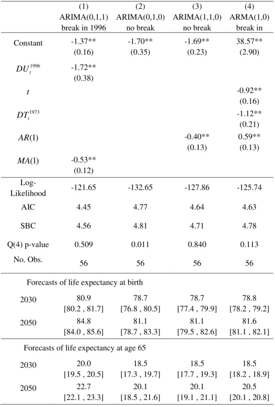
According to the results of the sequential testing approach the mortality index for the Portuguese males presents a structural change in 1996 and first-differences should be applied to induce stationarity. The appropriate model is then an ARIMA (0,1,1) model allowing for a structural change in 1996. Using this model we obtain forecasts of the mortality index for the period 2008 – 2050 and the corresponding 95% confidence bands. The confidence bands widen over time as a direct consequence of the unit-root non stationary model.

The impact of allowing for a structural change in the mortality index is illustrated by comparison of the above model with three other models estimated with different specifications of the structural change and the unit-root: (1) ARIMA (0,1,0) with drift or random walk with drift model, (2) the ARIMA (1,1,0) not allowing for a break, and (3) the ARMA (1,0) allowing for a break in 1973.

(17)

For each of the estimated models, mortality index forecasts are used also to produce forecasts for the age-specific death rates and forecasts for the life expectancy at birth and at 65 years were calculated. The optimal model with a unit-root and a change in 1996 gives the highest projected gains in life expectancy during the next four decades. The confidence bands for the mortality forecasts and the amplitude of the confidence bands for the 2050 life expectancy forecasts are substantially smaller for the optimal model than for the unit-root models without allowing for a structural change, but larger when compared with the trend-stationary model with a break.

The paper concludes with a discussion of the results comparatively with several research studies that show evidence regarding changes in the rate of decline of the general level of mortality. The findings are in line with these results and the paper concludes that the testing procedures can be used to select the appropriate forecasting model in the context of Lee-Carter model. Future research paths point to allowing more than one latent mortality index in the model to capture dissimilar evolutions of mortality at different ages, as well as the possibility of considering more than one structural change.

1.2. Patterns of Mortality Decline in Portugal since 1950

This paper considers mortality improvement patterns in Portugal, over the period 1950 – 2007. The aim is to show how a detailed descriptive analysis of the patterns of mortality improvement can be used to benefit the formulation and validation of a parsimonious model for estimating mortality dynamics over age and time. To identify the major patterns in the evolution of mortality over time for different ages, detailed descriptive analysis and graphical visualizations of mortality data are explored, as well as the analysis of the fitting results from the Poisson Lee-Carter model applied to the whole 1950-2007 period and to different sub-periods, and results from an extended model adding a second order age-period term.

(18)

are patterns in male mortality that have not been fully captured by the model. Deviance residuals plotted against age show larger residuals at infancy and around the accident hump ages, suggesting that there are age-period interactions not captured by the model. The plot of deviance residuals versus year of birth shows some sort of ripple effect, which suggest that not only period effects may differ between ages but also cohort effects may be influencing the mortality pattern.

The descriptive analysis of age-specific mortality rates, as well as composite longevity indicators such the life expectancy at birth, show that the rate of mortality decline at infant and younger ages has changed dramatically, and improvements at other ages have also had several distinct decline patterns over the period 1950 - 2007. In the case of male population, there are even periods of some deterioration in mortality conditions for some age groups. These differences in sensitivity of age-specific mortality to a temporal trend are not properly captured by the Lee-Carter model, and suggest that additional parameters should be added to the demographic model to allow for greater flexibility.

The findings concern the relevance of descriptive analysis for the specification of the model that most adequately captures mortality patterns. The Lee-Carter model with a second age-period interaction term is found to be the most appropriate model, however with less significant improvement for females than for males, and still, in the case of male mortality, some patterns are not fully captured. The possibility of a cohort effect is left for further research.

A succinct summary of each section of the paper follows.

(19)

of the distribution of deaths and the consequent rectangularization and expansion of the survival curve.

The third section of the paper briefly reviews the classical Lee-Carter method (Lee and Carter, 1992), and its Poisson extension proposed by Brouhns, et al. (2002), which assumes a Poisson distribution for the number of deaths and proposes a maximum likelihood interative estimation process. The latter is used in the empirical modelling. The addition of a second bilinear age-period term, which allows for a greater flexibility in capturing the mortality patterns, is also considered, following the work of Booth et al. (2002) and Renshaw and Haberman (2003). Model performance measures,

based on residuals, are discussed, such as the deviance residuals and the pseudo 2

R ,

proposed by Cameron and Windmeijer (1997) for Poisson regression models.

Section 4 presents and discusses the estimation results of the Poisson Lee-Carter model, applied for males and females separately, to the whole 1950 – 2007 period. In general the model captures the overall trends in mortality, the exceptions being those ages with a less regular behaviour where some difficulties of adjustment are evident, as in the case of men between 20 to 35 years old. Systematic pattern in the deviance residuals are visible, in particular for men, presenting a structure hardly consistent with the assumption of independence of the residuals, showing a diagonal clustering of residuals which suggest the presence of cohort effects.

The results of fitting the Poisson Lee-Carter model to four subsequent sub-periods, to address the problem of age-specific changing patterns, are presented in section 5. The results confirm that the rates of mortality improvement at each age have changed over time.

In section 6, the paper presents the results of the Lee-Carter model with a second age-period interaction term applied to the entire period 1950 – 2007. Overall, adding a second age-period interaction term improves the fit of the model, in particular for men by capturing the nonlinearity in the log-rates in particular at young ages. The impact of the second bilinear term for women is less significant. The analysis of the residuals for males, however, continues to show some clustering patterns.

(20)

captures mortality patterns is acknowledged. The possibility of a cohort effect in the male mortality is left for further research.

1.3. Cohort Effects in Mortality Modelling

This paper studies the possibility of a cohort effect in male Portuguese mortality, using period-cohort models, considering additive period and cohort effects as well as age-period and age-cohort interactions. The purpose of age-age-period-cohort models is to estimate the respective contributions of the effects of age, period and cohort on the evolution of the overall mortality. All three types of effects are distinct, but operate simultaneously, given the relation among them, which poses the problem of identification at the core of age-period-cohort modelling.

It is useful to define the three types of effects in age-period-cohort analysis. Age represents the intrinsic mortality risks related to biological and physiological factors, which are associated to the aging process, and which affect equally all individuals of the same age, regardless of their generational experience and observation period. Period effects are environmental conditions common to a given time period that change the level of mortality risk at all ages. Cohort effects or generational effects represent the influence of past conditions on current mortality risks; these are attributable to the life course experience of a cohort.

(21)

Portugal have focused on the impacts of age and period, and relatively little is known about possible cohort effects.

The paper, using the Bayesian Information Criterion (BIC), concludes that an age, period and cohort model with period and cohort effects moderated by age - the Renshaw-Haberman model - is the most suitable model to describe Portuguese male mortality patterns from 1950 to 2007. These findings are consistent with previous descriptive findings. The paper also concludes about the validity of BIC in the selection of the most parsimonious and adequate model through a simulation procedure.

A concise summary of each section of the paper follows.

Following a brief introduction, the paper presents the theoretical framework of the Age-Period-Cohort (APC) modelling, based on data arrayed by age and period, with equal interval widths for age and period, which identify cohorts by the diagonal cells of the table.

First, it contemplates the additive APC model, the identification problem of the APC model, the constrained-based approach proposed by K. Mason, W. Mason, Winsborough and Poole (1973) to estimate and solve the identification problem, as well as more recent developments, in particular the approach of Kuang, Nilsen and Nilsen (2008). The introduction of age-period and age-cohort interactions in the model is presented next. This is illustrated by the Lee-Carter model (Lee and Carter, 1992; Brouhns, et al., 2002), the Renshaw-Haberman model (Renshaw and Haberman, 2006), and the Lee-Carter model with additive cohort effects.

(22)

The seminal work of K. Mason, W. Mason, Winsborough and Poole (1973), address the identification problem in the age-period-cohort model and, using a multiple classification framework, propose a constrained-based approach, based on a priori and theoretical knowledge, to estimate the age, period and cohort model parameters. Several other approaches to solve the identification problem of the APC model have followed, such as estimable functions of the parameters invariant to the particular constrain applied, among which second differences of age, period and cohort effects (Clayton and Schifflers, 1987). Using second order differences of the three effects as measures of curvature, Kuang et al. (2008) propose an alternative approach to the identification problem in the age-period-cohort model, which consists in transforming the design matrix so that curvatures (the second differences) of age, period and cohort are estimated directly along with the two linear components. Still the original parameters are obtained imposing identification restrictions on the parameters.

Either explicitly or not, attempts to solve the identifiability problem, and obtain estimates of the absolute values of the age, period and cohort effects, are ultimately based on some type of constraint. According to Clayton and Schifflers (1987) and Carstensen (2007) it is not possible to uniquely estimate the absolute effects of age, period and cohort, unless the researcher is willing to make some assumptions on the relative importance of the effects, since it is not achievable to surmount the problem of having two variables as well as their sum in the same linear model.

The introduction of age-period and/or age-cohort interactions may be a way of solving the identification problem, but also carry specific identification requirements that need to be attended. The Lee-Carter model (Lee and Carter, 1992) includes an age-period interaction, but no cohort effect. The Renshaw-Haberman model (Renshaw and Haberman, 2006) generalizes the Lee-Carter model adding an additional age-cohort interaction. The authors also generalize the Lee-Carter model to include an additive cohort effect.

(23)

graphical analysis is that besides aging changing effects, period and cohort effects may both be present in the data.

In section 4 the estimation results of the following models are presented: the age-cohort (AC) model, the age-period (AP) model, the age-period-cohort (APC) model, the Lee-Carter (LC) model, the Lee-Carter with additive cohort effects (LCC), and the Renshaw-Haberman (RH) model. The fitting quality of each model is checked through the graphical analysis of the deviance residuals plotted against age, calendar year and year of birth, and by the values of deviance and BIC.

The Renshaw-Haberman model, with period and cohort effects both moderated by age, is found to be the most suitable model to describe Portuguese male mortality patterns from 1950 to 2007. This result is consistent with our expectations from the exploratory analysis of male mortality pattern in Portugal over 1950 – 2007, showing different rates of improvement for different ages, and the fact that some birth cohorts showed particular poor mortality improvements over adulthood when compared to other generations. The evidence of the graphical analysis, as well as the results from the estimated models, allude to the existence of cohort effects influencing Portuguese male mortality data.

(24)

the respective age interaction terms will result in an over parameterized model. Conversely, the omission of an interaction term will result in spurious cohort effects.

References

Booth, H., Maindonald, J., and Smith, L. (2002). Applying Lee-Carter under Conditions of Variable Mortality Decline. Population Studies, 56, 325– 336.

Booth, H, Hyndman, R.J., Tickle, L., and Jong, P. (2006). Lee-Carter Mortality Forecasting: a Multi-country Comparison of Variants and Extensions.

Demographic Research, 15, 289 – 310.

Brouhns, N., Denuit, M., and Vermunt, J.K. (2002). A Poisson Log-linear Regression Approach to the Construction of Projected Lifetables. Insurance: Mathematics

and Economics, 31, 373-393.

Case, R.A.M. (1956). Cohort analysis of mortality rates as an historical or narrative technique. British Journal of Preventive and Social Medicine 10, 159 – 171.

Cameron, A. C., and Windmeijer, F. A. G. (1997). An R-squared Measure of Goodness of Fit for Some Common Nonlinear Regression Models. Journal of Econometrics, 77, 329 -342.

Carstensen, B. (2007). Age-period-cohort models for the Lexis diagram. Statistics in

Medicine 2007; 26: 3018-3045.

Clayton, D. and Schifflers, E. (1987). Models for temporal variation in cancer rates II: Age-Period-Cohort Models. Statistics in Medicine, Vol. 6, 469-481.

Coelho, E. and Nunes, L. C. (2011). Forecasting mortality in the event of a structural change. Journal of the Royal Statistical Society A 174, Part 3, pp 713-736.

Harris, D., Harvey, D.I., Leybourne, S.J. and Taylor, A.M.R. (2009). Testing for a Unit-root in the Presence of a Possible Break in Trend. Econometric Theory, 25, 1545-1588.

Harvey, D.I, Leybourne, S.J. and Taylor, A.M.R. (2009). Simple, Robust and Powerful Tests of the Changing Trend Hypothesis. Econometric Theory, 25, 995-1029.

(25)

Kuang, D., Nielsen, B. and Nielsen, J.P. (2008a). Identification of the age-period-cohort model and the extended chain-ladder model. Biometrika, 95, 4, pp.979 – 986.

Lee, R. and Carter, L. (1992). Modeling and Forecasting U.S. Mortality. Journal of the

American Statistical Association, 87(419), 659-675.

Mason, K. O., Mason, W. M., Winsborough, H. H. and Poole, W. K. (1973). Some Methodological Issues in Cohort Analysis of Archival Data. American

Sociological Review, Vol. 38, n. º2, pp. 242-258.

Murphy, M. (2010). Reexamining the dominance of birth cohorts effects on mortality.

Population and Development Review 36 (2): 365 -390.

Perron, P., and Rodríguez, G. (2003). GLS Detrending, Efficient Unit-root Tests and Structural Change. Journal of Econometrics, 115, 1-27.

Renshaw, A., and Haberman, S., (2003). Lee–Carter mortality forecasting with age specific enhancement. Insurance: Mathematics and Economics 33 (2), 255–272.

Renshaw, A. E., and Haberman, S., (2006). A cohort-based extension to the Lee-Carter model for mortality reduction factors. Insurance: Mathematics and Economics, 58: 556–570.

Shang, H. L., R. J. Hyndman, and H. Booth (2010). A comparison of ten principal component methods for forecasting mortality rates. Working paper 08/10. Department of Econometrics & Business Statistics, Monash University.

Willets, R.C. (1999). Mortality in the next millennium. Staple Inn Actuarial Society Meeting, 7 December 1999. Available at: http://www.sias.org.uk/.

Willets, R.C. (2004). The cohort effect: insights and explanations. British Actuarial

Journal, 10, 833-877.

Zivot, E. and Andrews, D.W.K. (1992). Further Evidence on the Great Crash, the Oil-Price Shock, and the Unit-Root Hypothesis. Journal of Business & Economic

(26)

2. FORECASTING MORTALITY IN THE EVENT OF A

STRUCTURAL CHANGE*

(*) Joint research with Luís Catela Nunes.

Published in the Journal of the Royal Statistical Society A (2011), 174, Part3, pp. 713-736.

Abstract

In recent decades, life expectancy in developed countries has risen to historically unprecedented levels driven by unforeseen declines in mortality rates. The prospects of further reductions are of fundamental importance in various areas. In this context, we consider the problem of forecasting future mortality and life expectancy in the event of a structural change. We show how recent advances in statistical testing for structural changes can be used to arrive at properly specified models for the general level of mortality in the context of the Lee-Carter model. Specifically, the results of tests for a change in the trend of the mortality index and for the presence of a unit-root are used to identify appropriate forecasting models. The proposed methodology is applied to post-1950 mortality data for a set of developed countries in order to test the usual assumption made in the literature of a sustained decline in mortality at roughly constant rates in this period. Structural changes in the rate of decline in overall mortality are found for almost every country, especially in male populations. We also illustrate how accounting for such a change can lead to a major impact in mortality and life expectancy forecasts over the next decades.

(27)

2.1. Introduction

Over the past decades, life expectancy in developed countries has risen to historically unprecedented levels. The prospects of further future reductions in mortality rates are of fundamental importance in various areas such as demography, actuarial studies, public health, social insurance planning, and economic policy. Over the last years, significant progress has been made in mortality forecasting (for a recent review see Booth, 2006). The most popular approaches to long-term forecasting are based on the Lee and Carter (1992) model. It describes the time-series movement of age-specific mortality as a function of a latent level of mortality, also known as the overall mortality index, which can be forecasted using simple time-series methods. Some of the advantages of this approach are its simplicity and the robustness of the forecasts when age-specific log-mortality rates decline linearly over time. The method was initially used to forecast mortality in the U.S., but since then it has been applied to many other countries, including Australia (Booth, Maindonald and Smith, 2002), Austria (Carter and Prskawetz, 2001), Belgium (Brounhs, Denuit and Vermunt, 2002), Brazil (Fígoli, 1998), England and Wales (Renshaw and Haberman, 2003a, 2003b), Japan (Wilmoth, 1996), Spain (Guillen and Vidiella-i-Anguera, 2005; Debón, Montes, and Puig, 2008), Sweden (Lundstrom and Qvist, 2004), the Nordic countries (Koissi, Shapiro and Högnäs, 2006), and the G7 countries (Tuljapurkar, Li and Boe, 2000).

The original Lee-Carter model has also received a number of criticisms (see the discussion in Lee and Miller, 2001) and several extensions have been proposed in the literature (see Booth and Tickle, 2008). One major issue concerns the stability of the model over time. Since the method is usually applied to long time-series there is a risk that important structural changes may have occurred in the past. And any neglected structural change in the estimation period may result in forecasts that have a tendency to deviate from the future realizations of the mortality index, leading to potentially large long-term forecast errors. Moreover, inaccurate modelling of past trends also compromises the estimation of the past variability of mortality, leading to further biases regarding the estimation of forecast uncertainty.

(28)

re-estimated their random walk with drift model for the mortality index for several shorter and more recent periods and concluded that there was some instability. As noted by Lee (2000), if one had used their method to extrapolate the mortality index backward in time, one would arrive at too high mortality rates for the beginning of the 19th century. Other studies also document that there has been a systematic overestimation of the projected mortality rates in many countries (Stoto, 1983, Koissi et al., 2006). In multi-country comparisons of several versions of the Lee-Carter method, Booth, Hyndman, Tickle, and De Jong (2006) and Shang, Hyndman, and Booth (2010) find significant differences in the forecasting performance when alternative fitting periods are used, providing evidence of changing trends in the mortality decline rate.

This paper considers the problem of forecasting future mortality and life expectancy in the event of a structural change. We show how recent advances in statistical testing for structural changes can be used to arrive at a properly specified forecasting model for the general level of mortality in the context of the Lee-Carter model. Specifically, the results of tests for a change in the trend of the mortality index and for the presence of a unit-root are used to identify the appropriate model to be estimated and used to carry out the projections. In particular, it allows one to detect if a change is present or not, to estimate the date where the change occurs, and to determine if the appropriate forecasting model should be based on the levels or the first-differences of the mortality index series. The last distinction is important as the two alternatives lead to substantial differences in the amplitudes of the forecast confidence intervals.

(29)

according to our results, structural changes in the rate of decline in the overall mortality rate are found for almost every country considered and especially in the male populations. We consider as an example the case of Portuguese male mortality and show that accounting for a structural change leads to a major impact in mortality and life expectancy forecasts over the next decades.

The article is organized as follows. Section 2 presents a brief review of the Lee-Carter method and its extensions. The proposed approach to forecast mortality in the presence of structural change is described in Section 3. The empirical application is presented in Section 4. Finally, Section 5 discusses the results obtained and presents some concluding remarks.

2.2. The Lee-Carter Method

The Lee-Carter method combines a demographic model of age-specific death rates with statistical time-series forecasting methods. In this section, we give a brief description of the implementation of these two components of the method. We also present the Poisson regression extension that we follow in our empirical application.

2.2.1. The demographic model

The core assumption behind the Lee-Carter (1992) model is that the evolution of death rates for any age x is driven by a common time-varying component, denoted by

t

k , which is also referred to as the overall mortality index. More precisely, the

following relation is assumed:

( )

t k

( )

t

m_x =α_x+β_x _t+ε_x

ln (1)

where m_x

( )

t is the central death rate for age x and calendar year t, αx are the

age-specific parameters that affect the overall level of lnmx

( )

t over time, βx are the

age-specific parameters that characterize the sensitivity of lnm_x

( )

t to changes in the

(30)

historical influences not explained by the model. These errors are assumed to have zero mean and constant variance. Lee and Carter estimate the age-specific death rates by the following ratio:

( )

t x

t x x

E D t m

, ,

ˆ = (2)

where Dx,t denotes the number of deaths recorded at age x during year t from a

corresponding exposure-to-risk Ex,t.

Lee and Carter (1992) propose a two-stage procedure to estimate the model

given by equation (1). First, a least-squares solution to estimate αx, βx, and kt is

found. Since the model is clearly underdetermined, some normalization constraints are

imposed to obtain a unique solution: the sum of the βx over all ages equals one and the

sum of the kt over time equals zero. As a consequence, the αx will be equal to the

average values of lnmˆ_x

( )

t over time. The solution is found using the singular value

decomposition. Since the model is written in terms of log mortality, the observed total number of deaths in each year will not equal the sum of the fitted deaths by age. To

ensure this equality, the kt are estimated a second time, taking the αx and βx estimates

from the first step, such that for each year t, given the actual age distribution for the population, the implied number of deaths equals the observed number of deaths.

The homoskedasticity assumption on the error term εx

( )

t , implied by the

singular value decomposition estimation of the parameters αx, βx, and kt, has been

considered fairly unrealistic (Wilmoth, 1993; Alho, 2000) since the logarithm of the age-specific death rate is much more volatile at old ages, where the number of deaths and of those exposed to risk are relatively small. To circumvent this problem, Brouhns, Denuit and Vermunt (2002) propose an alternative model that keeps the Lee-Carter log-bilinear functional form, but replaces the least-squares approach with a Poisson regression for the number of deaths. Specifically, they consider the following model

describing the distribution of Dx,t:

( )

(

E t

)

Poisson

(31)

where the parameters αx, βx, and kt retain the meaning originally attributed by the

Lee-Carter model, and where µ_x

( )

t denotes the force of mortality. Note that if the force

of mortality is assumed to be constant within bands of age and calendar years, but allowed to vary from one band to the other, that is

( )

t _x

( )

t

y

x τ µ

µ ₊ + = for 0≤ y,τ <1, (4)

it follows that the force of mortality is identical with the central death rate,

( )

t m_x

( )

t

x =

µ .

The parameters of the Poisson model can be estimated by maximum likelihood

still subject to the model identification constraints that the sum of the βx over all ages

equals unity and the sum of the kt over time equals zero. The second stage in the

estimation of the kt, required in the classical Lee-Carter model, is no longer necessary

with this Poisson model since the sum of the estimated number of deaths by age will

automatically equal the total observed deaths in each year. Note that, although we use

the same notation for kt in equations (1) and (3), the estimates obtained from the

Lee-Carter and the Poisson regression will in general be different. Examples of the

application of the Poisson model are Brouhns et al. (2002) for Belgium, Renshaw and

Haberman (2003b) for England and Wales, and Koissi et al. (2006) for the Nordic

countries.

Given the estimated αx and βx in equation (1) or (3), the problem of forecasting

age-specific mortality rates and, consequently, life expectancies, is reduced to

forecasting the mortality index kt. This is considered in the following subsection.

2.2.2. Modelling the index of mortality

Lee and Carter (1992) propose using the Box-Jenkins methodology to arrive at

an appropriate ARIMA model to forecast the mortality index. In that methodology, the

first step always consists of determining if some transformation of the series is

necessary to induce stationarity before identifying and estimating the forecasting model.

(32)

ARMA(p,q) model fitted to the first-differences of the mortality index. For instance, an ARIMA(0,1,0) is adopted in the Lee and Carter (1992) study of U.S. mortality and in Tuljapurkar et al. (2000) for the G7 countries, and an ARIMA(1,1,0) is selected in Renshaw and Haberman (2003a) for England and Wales. Series whose first-differences are stationary are also called difference-stationary, and are described by a unit-root in their autoregressive representation. The usual approach to check this is by analysing the behaviour of the empirical autocorrelation functions. However, it is also possible to use formal statistical tests. The most popular are variants of the original Dickey and Fuller (1979) tests for the presence of a unit-root.

For illustration, consider an ARIMA (0,1,0) model, that is, a random walk with drift:

t t

t k d u

k − ₋₁ = + , (5)

where the drift d gives the mean annual change in kt, and ut are i.i.d. errors. The drift d

is estimated as the time-average of the series of first-differences ∆ = −kt kt kt−1. Given

any initial value for kt, this model implies that:

s t t

t s

t k ds u u

k₊ = + + ₊₁+ + ₊ , (6)

that is, future values of the mortality index equal the sum of a deterministic linear trend

component with slope d, given by the term kt+ds in equation (6), plus an error

component given by the sum of several shocks u. Since part of the uncertainty when

forecasting kt+s comes from the cumulative sum of the shocks, ut+1+ +ut s+ , it follows

that the forecast uncertainty grows with the forecast horizon s. It is straightforward to show that this result also holds for any other ARIMA(p,1,q) model.

If for a particular mortality index series the unit-root/difference-stationary hypothesis is rejected, the alternative hypothesis that should be considered would be that of stationarity around a linear trend capturing the linear decline in mortality. In such a case, the mortality index would be described by the following trend-stationary model:

t

t d d t u

k = ₀ + ₁ + , (7)

(33)

context of a generalized linear modelling version of the Lee-Carter model. Since model (7) is specified and estimated in the levels of kt, not the first-differences, it will in general produce forecasts that are different from the previous unit-root model. Also, given that in this model the deviations from the linear trend, given by ut, are stationary, the forecast uncertainty will no longer have a tendency to increase with the forecast horizon.

Unfortunately, the usual procedures based on the analysis of the autocorrelation function or on unit-root tests to decide about the appropriate class of forecasting model to be used, are only valid if the linear trend, and in particular the trend slope, d in model (6) or d1 in model (7), has remained constant over time. In the next section we discuss in more depth the implications of the presence of a structural change in the trend of the mortality index and propose a suitable approach to cope with this possibility when forecasting the mortality index.

2.3. Allowing for a Structural Change

A large literature on structural change models has emerged in the last years (see the surveys by Perron 2006, 2008). An important result is that, when producing long-term forecasts, any neglected or wrongly placed structural change occurring in the estimation phase may result in forecasts with a tendency to deviate from the future realizations of the series, resulting in potentially large forecast errors. It is also known that the correct approach to test for and estimate a model with a structural change is highly dependent on the stationarity properties of the time-series process.

(34)

although this option is not available in the latest version of the program (version 3.4.3). However, the method performs badly in the presence of strong positive autocorrelation (see Kim et al., 2000). Moreover, it is not valid in the presence of a unit-root, as is the case of any ARIMA(p,1,q) process, since it will lead to spurious breaks (see Nunes et al., 1996).

On the other hand, if it is known that the kt series is non-stationary with a unit-root, first-differences should be used instead. In general, the results obtained by following these two alternatives can be quite different in terms of a presence or not of a structural change and, in case one is detected, in terms of its dating.

In the literature of mortality forecasting, there are also some examples of approaches to account for the possible occurrence of a structural change. Booth et al.

(2002) find some evidence that the decline in the mortality index kt is not linear in their application of the Lee-Carter model to Australia, and try to avoid producing biased forecasts by selecting a best fitting period that insures linearity of the trend component assuming a unit-root. The criterion used is based on the ratio of a measure of the lack of fit of the model imposing a constant coefficients ARIMA model to the overall lack of fit of the Lee-Carter model. Lack of fit of the models are measured by mean deviance statistics. The chosen fitting period is that for which this ratio is substantially smaller than for periods starting in previous years. Denuit and Goderniaux (2005) also propose a similar solution, but assuming stationarity of the error term. The optimal starting year is determined by maximizing the R2 statistic for a linear regression as in equation (7). Therefore, both methods make an a priori assumption about the existence, or not, of a unit-root. Moreover, for both methods, the decision about the existence of a structural change and of its location, rely on non-objective criteria based on visual inspection of the time plots of model fit ratios or the R2. Another disadvantage is that since a specific fitting period is chosen, all information before the selected starting year is discarded. Therefore, these methods do not use all the available information available to estimate the variability of past mortality which is essential for instance in producing reliable forecast confidence intervals.

(35)

by Perron (1989), these approaches are not valid if a structural change is present, as they have a tendency to wrongly suggest a unit-root when the series is, in fact, stationary around a broken trend. As a solution, Perron (1997) proposes a modified unit-root test that is valid in the presence of a structural change at a known date. Zivot and Andrews (1992), Perron and Rodríguez (2003), and other authors have extended the test to the case where the change date is not known and must be estimated. However, when no change is actually present, several problems arise. As shown in Harris, Harvey, Leybourne, and Taylor (2009) (henceforth HHLT) there will be severe efficiency losses. Moreover, the estimated change date suggested by these tests may be spurious since, as shown by Nunes, Kuan, and Newbold (1995), the presence of a unit-root may lead one to erroneously find a structural change when there is none. In fact, when using the Zivot and Andrews (1992) unit-root test, the estimated change date is not even consistent for the true date if a change does occur. An example where such an inappropriate approach is followed is Chan, Li, and Cheung (2008) in a study of mortality in Canada, England and Wales, and the United States. Another issue is that the correct critical values to implement these tests become dependent on whether a structural change is present or not.

(36)

2.3.1. Testing for a change in the trend

As mentioned above, we use the HLT test for the existence of a structural change in the trend of the mortality index kt when it is not known a priori if the series has a unit-root or not. The date of the break, if present, is estimated from the available sample. The test is relatively simple to implement since it only requires estimating the following two linear regression models by least squares:

kt = α + β t + γDTt(τ) + ut , t = 1, …, T, (8) and

∆kt = β + γDUt(τ) + ut, t = 2, …, T, (9) where the change dummy variables are defined as DTt(τ) = t-TB if t > TB and DTt(τ) = 0 if t ≤ TB, DUt(τ) = 1 if t > TB and DUt(τ) = 0 if t ≤ TB, with TB = [τT] denoting the possible trend change date, and τ the associated change date fraction with τ ∈ (0, 1). Equation (8) corresponds to the trend-stationary case with stationary shocks ut and kt fluctuating around a linear trend with slope β subject to a change of magnitude γ occurring at a given date TB. Equation (9) corresponds to the case where the shocks to kt are non-stationary with a unit-root, so that the first-differences, ∆kt = kt - kt-1, fluctuate around the mean, given by the drift parameter β which is also subject to a change of

magnitude γ occurring at date TB. In this last equation, the shocks ut to ∆kt are also stationary. In both equations, the null hypothesis of no change in the trend slope corresponds to H0: γ = 0. The model described here corresponds to Model A in HLT. It is straightforward to allow for a simultaneous change in the slope and the level of the trend (Model B in HLT) by including an extra dummy variable in each regression. However, if the mortality index does not show any abrupt changes in its level, it is not necessary to consider such a model.

(37)

but may be inferred from the data itself, the test statistic is computed by the maximum of the sequence of t0(τ) statistics for all possible change fractions τ as:

t0* = supτ∈Λ | t0(τ) | (10) where the supremum is taken over a set Λ = [τL, τU ], with 0 < τL < τU < 1. HLT suggest setting the trimming parameters τL and τU equal to 0.1 and 0.9 respectively. Allowing for structural changes too close to the beginning or the end of the sample may lead to erroneous conclusions on the existence of a structural change in the trend since there may not be enough observations to support it. In our application presented in Section 4, this corresponds to the first five and last five observations in the sample. Li and Chan (2005) in a study of outliers also mention that the identified type and the estimation of an outlier may not be reliable when it lies within the last five observations of the series.

On the other hand, if it is known that kt is difference-stationary, one should use the corresponding t-statistic from equation (9), which we denote as t1 (τ). As in the previous case, given that the change date is not known a priori, the test statistic is given by

t1* = supτ∈Λ | t1(τ) |. (11) The change fractions at which the test statistics t0* and t1* attain their maximum will be denoted as τ0* and τ1*, respectively.

Finally, the HLT test, which is valid for both unit-root and trend-stationary processes, is computed as a weighted average of the t0* and t1* tests:

t_λ* = λt0* + m (1-λ ) t1* (12) with the weight λ given by

λ = exp[ - ( 500 S0*S1* )2 ] (13) and S0* and S1* denoting the KPSS (see Kwiatkowski, Phillips, Schmidt, and Shin, 1992) stationary test statistics calculated from the OLS residuals of equations (8) and

(9) when evaluated at the τ0* and τ1* change dates respectively. As shown in HLT, λ converges asymptotically to 1 if the series is trend-stationary or to 0 if it is difference-stationary at sufficiently fast rates so that the correct test statistic, t0* or t1* respectively, is selected. As shown by HLT, the 5% asymptotic critical value of tλ* equals 2.563

(38)

2.3.2. Unit-root test

As mentioned above, standard unit-root tests have several shortcomings when it is not known a priori if a structural change has occurred or not. However, as shown in HHLT, the HLT t_λ* structural change test in (12) can be used as a pre-test. If it rejects the null hypothesis of no change, an optimal test for a unit-root in the presence of a structural change should be used. If it does not reject, then an optimal unit-root test without allowing for a structural change should be used. We now describe these unit-root tests in more detail.

For the case where a structural change is detected with the HLT test, the estimated change fraction using the first-differenced model, τ1*, is used to estimate model (8) by GLS as in Perron and Rodriguez (2003). For τ = τ1*, equation (8) can be rewritten as

kt = Xt(τ1*)θ0 + ut , t = 1, …, T, (14) where Xt (τ1*) = (1, t, DTt (τ1*)) and θ0 = (α , β , γ )´. The GLS estimation is implemented by estimating with OLS the following quasi-difference transformation of equation (14):

kc,t = Xc,t(τ1*)θ0 + uc,t , t = 1, …, T, (15) where kc,t = kt - ρ kt-1 and Xc,t (τ1*) = Xt (τ1*) - ρ Xt-1 (τ1*) for t = 2, …, T, kc,t = k1 and Xc,t (τ1*) = X1 (τ1*) for t = 1, and ρ = 1- c/T where c is the quasi-difference parameter. The value of c can be chosen according to a local power criterion as explained in HHLT. Let

ˆ

c

θ denote the OLS estimator of θ0 in equation (15) and ut= kt - Xt(τ1

*

) ˆθc the residuals.

The unit-root test is finally obtained by estimating the following ADF regression:

1 ,

1

, 2,...,

p

t t j t j p t

j

u φu₋ δ u₋ e t p T

=

∆ = +

∑

∆ + = + . (16)

The number of lags p can be chosen by a modified Akaike criterion (see HHLT for details). Values of c and critical values for several significance levels and estimated change fractions needed for the implementation of this test can be found in HHLT and Carrion-i-Silvestre, Kim, and Perron (2008).

(39)

Elliot, Rothenberg, and Stock (1996). This test is computed as above but with the following two modifications: a) the structural change dummy variable is excluded from the Xt(τ1*) vector and b) the optimal value of c in this case equals 13.5.

2.4. Empirical Application

In this section, the methodology proposed above is illustrated by an application to the following 18 developed countries: Austria, Belgium, Canada, Denmark, England and Wales, Finland, France, Ireland, Italy, Japan, Netherlands, Norway, Portugal, Spain, Switzerland, Sweden, United States of America, and West Germany. These countries experienced large increases in life expectancy during the twentieth century, interrupted only by the global influenza epidemic in 1918-19 and the two World Wars (Bongaarts, 2006). However, the decline in mortality rates was not simultaneous in all countries, and rather diverse situations prevailed until the Second World War (Monnier, 2004). The increases in life expectancy were more pronounced during the first half of the century, affecting in particular early ages in life (Wilmoth, 2000). The pace of improvement in life expectancy slowed down around the middle of the century, when the predominant types of mortality reduction shifted from curing infectious diseases that heavily affect the young to degenerative diseases that largely affect the elderly (see White, 2002, and Vallin and Meslé, 2004). Several studies also provide evidence that the age pattern of mortality decline changed over time (e.g. Kannisto, Lauritsen, and Thatcher 1994; Horiuchi and Wilmoth, 1998; Wilmoth, 1998; Carter and Prskawetz, 2001; Lee and Miller, 2001).

(40)

We use time-series data obtained from the Human Mortality Database (HMD), sponsored by the University of California, Berkeley, and the Max Planck Institute for Demographic Research (http://www.mortality.org), for the number of deaths, Dx,t, and

exposure-to-risk, Ex,t, by single year of age, sex, and calendar year from 1950 (for

West Germany data are available only since 1956) until the most recent available year (2005 for Austria, Canada, and U.S.A., 2006 for Belgium, England & Wales, France, Ireland, Italy, Netherlands, Spain, and West Germany, and 2007 for Denmark, Finland, Japan, Norway, Portugal, Switzerland, and Sweden). The Ex,t are based on annual population estimates with a small correction that reflects the timing of deaths during the interval (see HMD, 2007).

We first apply the Brouhns et al. (2002) Poisson regression extension of the Lee-Carter method described in Section 2 to obtain estimates of the model parameters and the mortality index series for the male and female populations in each country. Next, we apply the procedure proposed in Section 3 to test for the presence of structural changes and unit-roots in the estimated mortality indices. We note that the proposed procedure does not affect the estimation of the kt. Finally, we illustrate how these results can be used to arrive at appropriate forecasting models by considering the case of male mortality in Portugal. We compare the resulting mortality and life expectancy forecasts with those obtained using alternative models.

2.4.1. Estimation of the index of mortality

The estimated mortality indices k_t for the male and female populations in each

(41)

Austria

-100 -50 0 50 100

1950 1960 1970 1980 1990 2000

Males Females

Belgium

-100 -50 0 50 100

1950 1960 1970 1980 1990 2000

Males Females

Canada

-100 -50 0 50 100

1950 1960 1970 1980 1990 2000

Males Females

Denmark

-100 -50 0 50 100

1950 1960 1970 1980 1990 2000

Males Females

England & Wales

-100 -50 0 50 100

1950 1960 1970 1980 1990 2000

Males Females

Finland

-100 -50 0 50 100

1950 1960 1970 1980 1990 2000

Males Females

(42)

France

-100 -50 0 50 100

1950 1960 1970 1980 1990 2000

Males Females

Ireland

-100 -50 0 50 100

1950 1960 1970 1980 1990 2000

Males Females

Italy

-100 -50 0 50 100

1950 1960 1970 1980 1990 2000

Males Females

Japan

-150 -100 -50 0 50 100 150

1950 1960 1970 1980 1990 2000

Males Females

Netherlands

-100 -50 0 50 100

1950 1960 1970 1980 1990 2000

Males Females

Norway

-100 -50 0 50 100

1950 1960 1970 1980 1990 2000

Males Females

Modelling and Forecasting Mortality Patterns

Instituto Superior de Estatística e Gestão da informação

Universidade Nova de Lisboa

Modelling and Forecasting Mortality Patterns

Instituto Superior de Estatística e Gestão da informação

Universidade Nova de Lisboa

Modelling and Forecasting Mortality Patterns

ACKNOWLEDGMENTS

ABSTRACT

RESUMO

CONTENTS

1.

INTRODUCTION

2.

FORECASTING MORTALITY IN THE EVENT OF A

STRUCTURAL CHANGE*

( )

( )

( )

( )

( )

( )

( )

( )

( )

(

)

( )

( )

( )

( )

( )

∑