i
António Augusto Mousinho Almadanim Santa
Marta
Degree in Environmental Engineering Sciences
Sustainable Aquaculture in Saldanha Bay,
South Africa
Dissertation submitted to obtain the degree of Master in Environmental Management Systems
Thesis advisor: João Gomes Ferreira FCT-UNL
Jury:
President: João Gomes Ferreira External examiner: João Lencart e Silva Internal examiner: António Carmona Rodrigues
iii
António Augusto Mousinho Almadanim Santa
Marta
Degree in Environmental Engineering Sciences
Sustainable Aquaculture in Saldanha Bay,
South Africa
Dissertation submitted to obtain the degree of Master in Environmental Management Systems
Thesis advisor: João Gomes Ferreira FCT-UNL
Jury:
President: João Gomes Ferreira External examiner: João Lencart e Silva Internal Examiner: António Carmona Rodrigues
iv Copyright © António Augusto Mousinho Almadanim Santa Marta, Faculdade de Ciências e Tecnologia, Universidade Nova de Lisboa
v
AKNOWLOGMENTS
First of all, I want to thank my professor and thesis advisor Prof. João Gomes Ferreira for the opportunity, the guidance, motivation, time spent, and availability. I have learned a lot with him. I would like to express my very great appreciation to Dr. Grant Pitcher for the crucial data, the kind help in reading and constructively criticizing my draft thesis, the precious support, and time spent.
I would like to thank Dr. Sue Jackson for the kind availability, crucial help with data and contacts. I also want to thank Mr. Schalk Visser, Mr. Vos Pinaar, and Mr. Kevin Ruck for the availability and kind help with important data.
Thank you to my family for the patience, love, and comprehension.
I would like to offer my special thanks to my mother for the friendship, crucial support, and kind help.
Thank you to my thesis companions Rita Pinto, João Mello, and José Pedro Vieira, for all company and support.
Manny thanks to my very good friend André Pataco for the companionship, important help, and support along this period.
vii
ABSTRACT
Saldanha Bay, located near the coastal town of Saldanha, in Western Cape Province of South Africa, possesses excellent conditions for mussel and oyster aquaculture. Its linkage with the adjacent upwelling current system provides a very productive environment for phytoplankton growth, and this has led to the development of a vibrant shellfish aquaculture industry. The main objectives of this work are to develop a model which simulates the main ecological processes within the Bay, to determine the Bay’s carrying capacity for mussel and oyster production, and to produce a management tool for decision making.
Bivalve aquaculture has great growth potential and may be important for human food security as mankind faces a projected need of an additional 30 X 106 tonnes per year of aquatic products by 2050. Bivalve aquaculture is organically extractive, and can additionally provide significant ecosystem services in top-down control of eutrophication, and creation of structure for stimulating biodiversity. When managed properly, this form of aquaculture has a very low environmental footprint, mainly associated with organic enrichment of the sediment. This impact is even less relevant in upwelling systems such as Saldanha Bay where particles tend to be flushed out in the surface layer, and in all cases it must be borne in mind that by definition shellfish aquaculture results in a net removal of seston from the water column.
This model was developed using EcoWin an object oriented approach to ecological modelling. The model for Saldanha Bay was set up using oceanographic and water quality data collected from Saldanha Bay, and culture practice information provided by local shellfish farmers. The first step was the construction and calibration of the ecological model, in order to provide a general description of the biogeochemical behaviour of the Bay, followed by the addition of the shellfish aquaculture component.
EcoWin successfully reproduced the key ecological processes, correctly simulating a mean phytoplankton biomass of 7.5 chl a L-1. The aquaculture module simulated an annual harvested biomass of about 3000 t y-1, in good agreement with reported yield.
Six production scenarios were explored, for illustrative purposes: - Increase in stocking density of shellfish
- Two alternatives for aquaculture development in particular areas of Saldanha Bay - Prediction of the maximum production capacity of the Bay.
ix
Table of contents
1 Introduction ...1
1.1 Carrying capacity ...2
1.2 Aquaculture potential...3
1.3 Aquaculture ...4
1.4 Aquaculture around the world...5
1.5 Importance of site selection for Aquaculture in Africa...6
1.6 Shellfish aquaculture...6
1.6.1 Impacts of Shellfish aquaculture ...7
1.7 Production methods ...9
1.8 Oyster and Mussel biology ...9
1.8.1 Mussels ... 10
1.8.2 Oyster... 11
1.9 Legal Framework ... 11
1.9.1 Health and safety regulation ... 12
1.9.2 General policy... 12
1.10 Physical description of Saldanha Bay ... 13
1.11 Use conflicts ... 15
1.12 Carrying capacity studies ... 15
1.13 Bivalve studies in Saldanha Bay ... 16
2 Methods ... 19
2.1 Tools used... 21
2.2 Data... 22
2.3 The Hydrodynamic model ... 23
2.4 Forcing Functions ... 24
2.5 Temperature ... 25
2.6 Salinity ... 26
x
2.8 Nutrients ... 28
2.9 Suspended Matter ... 29
2.10 Phytoplankton ... 30
2.11 Parameters ... 31
2.12 Shellfish... 33
3 Results and Discussion ... 37
3.1 Water temperature ... 37
3.2 Salinity ... 38
3.3 Dissolved Inorganic Matter ... 38
3.4 Phosphate... 40
3.5 Suspended Particulate Matter ... 41
3.6 Particulate Organic Matter... 42
3.7 Phytoplankton ... 42
3.8 Ecological model discussion... 44
3.9 Model validation – Standard Scenario ... 45
3.10 Carrying capacity ... 50
3.10.1 Production carrying capacity ... 50
3.11 Production scenarios: ... 55
3.11.1 Scenario 1 ... 55
3.11.2 Scenario 2 ... 56
3.11.3 Ecological impacts – Scenario 1 and 2 ... 56
3.12 Scenario discussion... 58
4 Conclusion ... 61
xii
LIST OF FIGURES
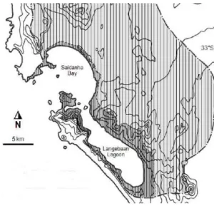
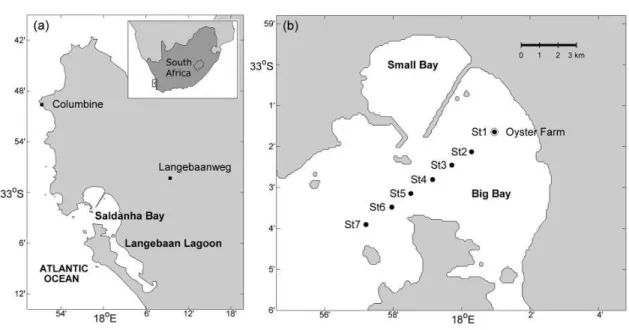
Figure 1 – Location of Saldanha Bay: 1) Southern Africa; 2) South Africa; 3) North from Cape
town; 4) Satellite view of Saldanha Bay. ...1
Figure 2 – Production methods illustration (left side) a tray method (right side); source: A. Figueras (2004). ...9
Figure 3 –Mytilus Galloprovincialis, shell illustration (left side) and picture (right side). Source: A. Figueras, (2004)... 10
Figure 4 – Crassostrea gigas shell illustration (left side) and picture (right side). Source: (Helm, 2005) ... 11
Figure 5 – Saldanha Bay illustration before iron ore construction. Source: B. W. Flemming, (1977)... 13
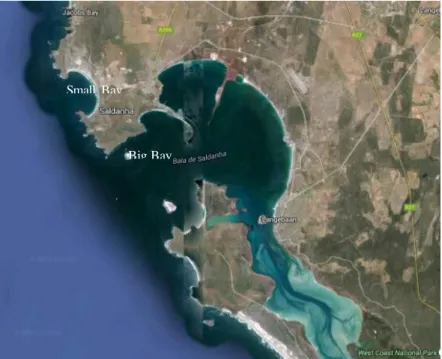
Figure 6 – Saldanha Bay actual satellite picture. Source: Google maps... 14
Figure 7 – Simplified modelling framework used... 19
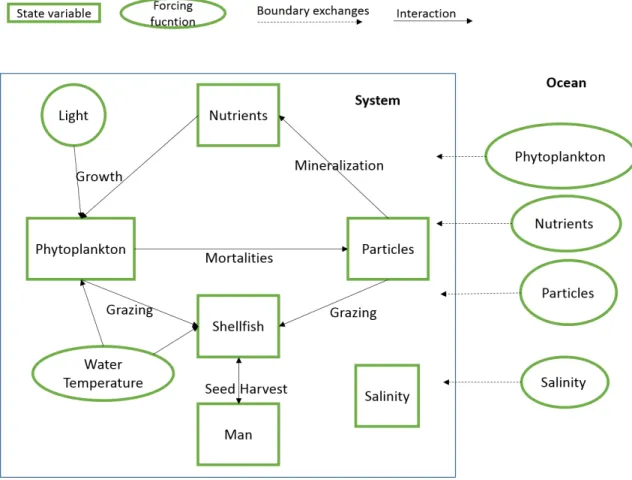
Figure 8 – Conceptual model schematization. ... 20
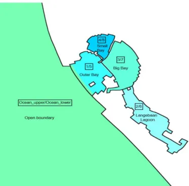
Figure 9 – Models box scheme organization. ... 21
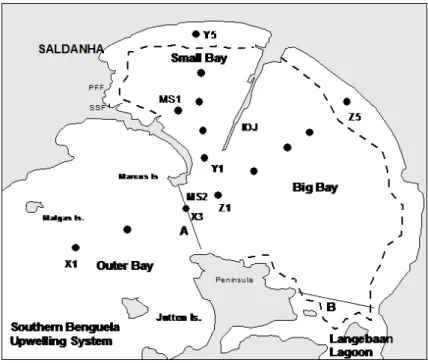
Figure 10 – Sampling stations spatial distribution inside the Bay. Source: Smith and Pitcher, (2015)... 22
Figure 11 – Sampling stations for particle matter spatial distribution. Source:Monteiro and Largier, (1999) ... 23
Figure 12 – Hydrodynamic model illustration. ... 24
Figure 13 – Temperature forcing functions used for each box. ... 26
Figure 14 – Ocean boundaries salinity curves. ... 27
Figure 15 – Boundary conditions for silica, phosphate, nitrite, nitrate and ammonia. ... 28
Figure 16 – SPM (left side) and POM (right side) boundary conditions. ... 30
Figure 17 – Boundary phytoplankton biomass. ... 31
Figure 18 – Temperature results for each box and measured data. ... 37
Figure 19 – Salinity results for each box. ... 38
Figure 20 – DIN results for each box. ... 39
xiii
Figure 22 – SPM results for each box... 41
Figure 23 – POM results for each box. ... 42
Figure 24 – Phytoplankton results for each box. ... 43
Figure 25 – Phytoplankton results for boxes 3 and 4. ... 43
Figure 26 – Standard scenario harvested weight for each species for each area ... 46
Figure 27 – Oyster individual weight evolution in box 3 (left side) box 4 (right side), mussel individual weight evolution in box 4 (bottom) ... 46
Figure 28 – Oyster individual weight for 3 different POM scenarios: standard model (mean 1.1 mg L-1 POM); case 1 (mean 1.3 mg L-1 POM); case 2 (mean 0.9 mg L-1)... 47
Figure 29 – Difference between phytoplankton biomass before and after adding shellfish farms to the model. ... 48
Figure 30 – Harvest results for different seeding intensities of mussel (left) and oyster (right), inside Small Bay ... 51
Figure 31 – Number of seeds in Small Bay for the two maximum scenarios ... 51
Figure 32 – Harvested shellfish in live weight and wet meat in tonnes for the maximum production scenarios in Small Bay... 52
Figure 33 – Oyster harvested weight per seeded weight inside Big Bay ... 53
Figure 34 – Comparison of harvested live and wet meat weight of oyster in Small and in Big Bay. ... 53
Figure 35 – Average phytoplankton biomass inside each box ... 54
Figure 36 – Comparison of maximum production capacity in each box ... 55
Figure 37 – Scenario 2 annual shellfish harvest. ... 55
Figure 38 – Scenario 2 oyster annual harvest in box 4. ... 56
xiv
LIST OF TABLES
Table 1- Nitrogen removal costs for different removal strategies, source: Ferreira and Bricker,
(2015)...7
Table 2 – Stations used for each box group. ... 25
Table 3 – Initial salinity conditions for each box. ... 27
Table 4 – Initial conditions for each box ... 29
Table 5 – Initial conditions for each box to POM and SPM ... 30
Table 6 – Initial phytoplankton biomass for each box... 31
Table 7 – Phytoplankton parameters used... 32
Table 8 – Suspended particle matter used parameters. ... 33
Table 9 – Companies working in Saldanha Bay, respective annual production and licensed area. ... 34
Table 10 – Mussel and oyster production, number of seeds, farm area, seed and harvested shellfish weight. ... 35
Table 11 – Comparison between measured average DIN and mean DIN results for each box. .. 39
Table 12 – Measured average phosphate comparison with mean results phosphate for each box. ... 40
Table 13 – Modelled and estimated production for each box, organized in species. ... 45
Table 14 – Bivalve ecosystem removals for each farmed box. ... 48
Table 15 – Mean phytoplankton comparison, before and after adding the farms into the model, in boxes 3, 4, 7, and 8. ... 49
Table 16 – Total scenario removal for each species and total ... 50
1
1
Introduction
The government of South Africa approved a National Development Plan, Vision 2030 that aims to reduce poverty, unemployment and inequality by this date. For the present government, “aquaculture’s role and contribution to food security is central to addressing poverty, unemployment, and inequality” (National Aquaculture Policy Framework, 2013).
The coastal Town of Saldanha, in South Africa, is located near a Bay which has excellent conditions for mussel and oyster culture. This Bay is home for farms of both species, with an annual total production of about 2400 tonnes. Saldanha Bay is located in the southwest coast of the country, forming part of the Benguela Current Large Marine Ecosystem. Due to the upwelling in Benguela current system, this Bay has nutrient rich waters, providing a productive environment for phytoplankton growth (Olivier et al., 2013).
2 The central question addressed in this thesis is whether the current farming activities are working at the Bay’s carrying capacity defined as the maximum production achievable without affecting the ecosystem, including other such as fisheries to an unacceptable level. This question is developed into four main objectives: (1) to analyse the carrying capacity of Saldanha Bay for shellfish production at the scale of the Bay; (2) to describe the main environmental variables and processes and their interactions with the aquaculture activities; (3) to develop different production scenarios; (4) to illustrate how ecological models can support management decisions for Saldanha Bay.
1.1
Carrying capacity
Carrying capacity has been interpreted in a range of different perspectives, such as, physical, social, economic and environmental. Davies and McLeod (2003), for instance, considered bivalve carrying capacity as “the potential maximum production a species or population can maintain in relation to available food resources” (production perspective) as Lindsay G. Ross et al. (2013) defined carrying capacity as “the level of resource use (…) that can be sustained over the long term by the natural regenerative power of the environment” (an ecological perspective). Inglis, G.J. et al. (2000) defined carrying capacity in the broader and more important perspective, considering that carrying capacity can be interpreted in four categories: physical, production , ecological and social carrying capacity;
With a similar perspective, FAO defined in 2013 an approach to aquaculture, which has three principles: (1) aquaculture development without degradation of the ecosystem beyond its resilience capacity; (2) improvement of human well-being and equity for all relevant stakeholders; and (3) development in the context of other policies, sectors, and goals.
3 The individual use of either ecological or production carrying capacity criteria is not adequate for shellfish farming management. The strict ecological perspective does not allow any change in the receiving environment and the production capacity does not consider any environmental criterion (Guyondet et al., 2010). A general carrying capacity should be a compromise between production and ecological carrying capacity (Gibbs, 2007; McKindsey et al., 2006), the ultimate goal must be the development of the most productive farm without compromising its long term viability nor the ecosystem stability (Guyondet et al., 2010). McKindsey et al. (2006), uses the definition of G.J. et al. (2000) to build a decision framework that integrates its four categories to determine the overall capacity for bivalve aquaculture. This framework uses physical carrying capacity, production carrying capacity, ecological carrying capacity and social carrying capacity, in this order. In this way it is possible to calculate the general carrying capacity for a certain location. This study intends to combine physical, production, and ecological carrying capacity concepts, using these methods. The generic carrying capacity should also include both local and system scale approaches (Smaal et al., 1997). The system scale is used to determine the propagation of local effects (Guyondet et al., 2010) and the local scale is used for farm management considerations (Ferreira et al., 2007; Strohmeier et al., 2008).
The importance given to sustainable development and consequently to ecological carrying capacity varies around the globe, for instance, the developing and underdeveloped countries are less committed to it (Aguilar-Manjarrez et al., 2010). Carrying capacity is a central concept in ecosystem-based management, as it avoids “unacceptable changes” in the natural ecosystem and social structures by setting upper limits to aquaculture considering environmental limits and social acceptability for aquaculture. It is very important to evaluate the carrying capacity to an area before establish large-scale shellfish farms, to ensure a suitable food supply for the expected production and to avoid and minimize ecological impacts (Ferreira et al., 2008).
1.2
Aquaculture potential
4 Fish have the highest protein content in their flesh of all food animals. They are more efficient than any terrestrial farmed animals, converting feed to body tissue. Besides all this, aquatic animals discharge two to three times less nitrogen to the environment when compared to terrestrial food production systems (Costa-Pierce, 2010).
1.3
Aquaculture
Aquaculture is the cultivation of aquatic organisms including finfish, shellfish, and plants. Cultivation involves the enhancement of natural production processes such as feeding, stocking, and protection from predators. The act of farming means that there is some kind of ownership, individual or corporate, over the stock (Handbook of Fishery Statistical Standards.).
Aquaculture can take place on land or in waterbodies; the latter include freshwater such as rivers or lakes, brackish water such as estuaries, and fully saline water such as Bays and open coastal water. In onshore aquaculture, ponds are most widely used for production. Cage based aquaculture for freshwater has bigger impacts. Although the use of ponds in brackish water faces substantial competition for space and environmental problems, ocean onshore production has developed in some areas where it wouldn’t be possible otherwise. The coastal floating cage farms have proved to be the most effective production system. The production of seaweed and marine molluscs has been developing since the 1990s to specialized techniques allowing it to grow significantly. (Bostock et al., 2010)
Growth of freshwater aquaculture is increasing pressures on natural resources, mainly water, feeds, and energy. Most freshwater aquaculture involves water intake from the environment and post-production effluent stream. Given the increasing pressures on fresh water supplies greater use of brackish and marine water is expected in the future (Bostock et al., 2010).
5 Most mollusc farming needs no feed inputs and the majority of freshwater fish production uses a low-protein, grain-based diets, and organic fertilizers. Much of the marine species crustaceans and other fish aquaculture use a higher quality diet usually containing fish meal and fish oil. Some aquaculture, such as tuna fattening needs small pelagic fishes. Although not essential, feeds for herbivorous and omnivorous species frequently contains fish meal and oil. The rapid expansion of carnivorous species could also increase pressure on fish meal and oil supplies. Overall the supplies of fish meal and oil won’t be sufficient to meet the increasing demands for aquafeed ingredients. Nevertheless this isn’t expected to be a great constraint, but the demand for alternative feed materials will increase. (Bostock et al., 2010)
There are several approaches to integrate aquaculture with other activities, such as, fisheries, agriculture, and Integrated Multi-Trophic Aquaculture (IMTA). Many aquaculture systems need captured fish for its feeds and aquaculture has an important role in fisheries capture enhancements, releasing farmed fish. Their release can however represent significant ecological and genetic risk to wild fish stocks.
The integration of fish species from different trophic levels can be made in the same water body or with some other water based linkage. This combination generates a synergetic relationship that acts as a bioremediation measure. A perfect system of this nature would be environmentally neutral. Such methods face a number of challenges, such as species selection, economic value , and existing regulations for aquaculture.
The integration of aquaculture and agriculture is most common in developing countries, as it diminishes the risks of mono culture. These systems use the synergy between systems to diversify production and to enhance productivity.
1.4
Aquaculture around the world
6 With few exceptions such as Norway, aquaculture development in developed countries is very limited. In these countries aquaculture growth has been limited by user conflicts, access to sites, complicated regulatory regimes, lack of government investment, consumer disinterest, and lack of aquaculture education. In the poorest nations, aquaculture development has not occurred significantly, except for, Bangladesh, India, Vietnam, and Egypt (Costa-Pierce, 2010).
1.5
Importance of site selection for Aquaculture in Africa
With the decline of fish stocks worldwide, aquaculture is looked at as an important solution, especially for Africa, in which many areas contain an undernourished population dependent on marine and freshwater fishing for incomes (Wit, 2013). The development of aquaculture needs to be planned in order to diminish environmental and social impacts, and to predict optimum production scenarios (Byron and Costa-Pierce, 2013). The use of GIS is the most efficient, cheap, and fast way to select sites for aquaculture. It involves the identification of economically, socially, and environmentally available areas (McLeod et al., 2002). The use of these models requires regional data and the costs of data collecting in the sea are often high. Given the economic panorama in most of the African countries, this kind of expenses can be a limiting factor. Therefore, use of remote sensing has great potential and importance to the use of GIS and in this region, to determine the viability of some projects and decision making (Wit, 2013).
1.6
Shellfish aquaculture
7 Bivalves may have an important role in the nutrient credit programs. There is an excess of nutrient inputs to the water in numerous areas of the European Union (EU) and North America, mostly from non-point sources. The concept of a nutrient credit program is to reduce the nutrient loads by using a market based approach. This approach uses economic incentives to reduce nutrient discharges, by attributing credits to the involved polluters, which they can sell if come to reduce their emissions. In this way, the ones who can reduce their emissions by a lower price can sell their remaining credits. This could create new monetary income opportunities for farmers, who can remove nutrients from the water at a low price, as table 1 shows. The shellfish nutrient removal is one of the cheapest methods of doing it as it has great potential. These programs are already in use in some parts of the US, although not in the EU nor African countries, such as South Africa.
Table 1- Nitrogen removal costs for different removal strategies, source:(Ferreira and Bricker, 2015)
Non-point-source nutrient management strategy Cost (euro kg-1 N)
Shellfish 11 – 278
Agricultural 0.2 – 870
Urban stormwater 56 – 6720
Wastewater treatment upgrades 0.9 – 14 093
Wetlands 1.1 – 396
Other 5.2 – 404
1.6.1
Impacts of Shellfish aquaculture
8 Many studies have been made to determine the impacts of bivalve farming. The biodepositon process results in the enrichment of organic materials in sediment and this may cause the reduction of the level of dissolved oxygen in the lowest layer, increase levels of sulphides, changes of benthic assemblages and azoic conditions (Zhang et al., 2009), resulting in the appearance of opportunistic species and biodiversity decrease in the substrate (Stenton-dozey et al., 1999). When close to the production carrying capacity, shellfish aquaculture may reduce the zooplankton availability, by over-compete it in phytoplankton consumption. This might reduce some higher trophic level fish, which would depend on zooplankton (Jiang and Gibbs, 2005), the introduction of exotic species and proliferation of certain species such as starfish and jellyfish are possible impacts as well (McKindsey et al., 2011).
Souchu et al. (2001) tested the effects of shellfish farming in the water column in Thau Lagoon in Mediterranean France. A nutrient surplus was observed in the water column near the farms, as a cause of plankton removal by shellfish. Thau Lagoon however, has very different physical conditions than Saldanha Bay, as a Mediterranean lagoon with low tides, wind, and wave events. Chamberlain et al. (2001), studied the effects of mussel farming on the surrounding sediments in Southwest Ireland in two different farms, and obtained different results for each. One (lower current speed) showed organic material enrichment and an impoverished benthic community as the other showed no significant impacts. Studies on suspended shellfish (mussels and oysters) culture in Tasmania (Crawford et al., 2003), and Nova Scotia (Grant et al., 1995) found little impact on the benthic community. Stenton-Dozey et al. (2001) studied the impacts of mussel farms in Saldanha Bay and found significant impacts on the substrate, such as anoxic conditions, presence of opportunistic polychaetes and a significant reduction in macrofaunal biomass. Zhang et al. (2009) studied the impacts of intensive shellfish and seaweed farming in Sanggou Bay, China and found some biochemical and biological changes, but these were considered low impact over a longer term. Kaspar et al. (1985) studied the impacts of mussel production in Kenepuru Sound, New Zealand and it found a strongly affected benthic community, with biodiversity reduction and a surplus of nitrogen in the water column.
9
1.7
Production methods
The main cultivated species in Saldanha Bay are the oyster Crassostrea gigas and the mussel Mytilus galloprovincialis, and constitute the focus of this study the two species are cultivated using similar techniques: raft culture; long-line culture; rack culture; on-bottom culture; and perforated plastic trays/mash bags. There are several variations of the same methods with different materials. Figure 2 illustrates some of these methods.
Figure 2 – Production methods illustration (left side) a tray method (right side); source: A. Figueras (2004).
Mussel seed can be collected manually or using collecting ropes where it attaches naturally, hatchery is not common for mussels. The mussels are afterwards grown on ropes, which can be suspended from rafts, wooden frames, or longlines of floating plastic buoys. Mussel can be harvested around the year, but this should be avoided during spawning periods.
Oyster seeds can be obtained through artificial collectors too or in hatcheries, which can force the animal spawning, having seeds available all year round. The oysters can be set in mesh bags or perforated plastic trays in the low intertidal zone, or in suspension ropes as with Mytilus galloprovincialis. They are also not harvested during the spawning period, for lower quality meat. (Aypa, n.d.; Garrido-Handog, n.d.)
1.8
Oyster and Mussel biology
10 The class Bivalvia is one of six Mollusc classes and includes all the animals enclosed in two shell valves, such as, the mussel, oyster, clam, and scallops. The shell serves as protection for predators, a skeleton for the attachment of muscles, and it helps to avoid mud and sand into the mantle cavity in burrowing species. Between bivalve species the shell’s form, colour, and markings diverge significantly.
Bivalves are filer feeders and feed mainly on phytoplankton, they have the ability to select the food filtered from the water. The food is bounded with mucous, passed to the mouth, and sometimes rejected and discarded out of the animal, when is named “pseudofaeces” (Helm et al., 2004).
1.8.1
Mussels
Mussels have two shells, similar in size and approximately triangular. Shell colour varies with age and location of the animal. The two shells are held and articulated together at the anterior through a ligament. The foot serves to attach the mussel to the substrate or other mussels, by the secretion of tough filaments in the ventral part of the mussel (Gosling, 2008).
Mussel length varies under the environmental conditions over which it lives. Under optimal conditions a mussel can reach a much bigger length than when exposed to marginal conditions. The shells of closely packed mussels have higher length to height ratios, from those in less crowded sites (Gosling, 2008).
The mussel species used for this study is Mytilus galloprovincialis, or Mediterranean mussel. These species live in waters with temperature ranging from 10 to 20°C, salinity around 34‰ psu. This species can reach up to 15cm but the normal length is 5-8cm. (Figueras, 2004). Figure 3 illustrates this species shell.
11
1.8.2
Oyster
The European flat oyster, Ostrea edulis, valves are roughly circular, one valve is flat and the other cupped, and they are hinged together by a tense ligament on the dorsal side. The flat side of the shell is attached to the substrate. The American Eastern oyster, Crassostrea virginica, has a more lengthened shape than the European one, and the upper shell more profoundly cupped. The shell is for both species thick and solid. In general the Ostrea edulis has a maximum shell height of 100mm as Crassostrea virginica ca reach 350mm length (Gosling, 2008).
The species studied in this work is Crassostrea gigas, also known as the Pacific oyster, originally from Japan. This bivalve is an estuarine species that prefers hard bottom substrate, from the lower intertidal area to depths of 40m. The optimal salinity range is 20 –25 ‰, but it can live in salinities between 10‰ psu and 35‰ psu. It tolerates temperatures from -1.8 to 35°C and it can achieve commercial size in 18-30 months when in good conditions. Its rapid growth and wide range of tolerance to environmental conditions, made this oyster the preferred choice for many farmers worldwide. This oyster has an elongated, cupped, and extremely rough shell, as Figure 4 illustrates. The maximum length is 30 cm, but the normal length ranges between 8 to 15 cm (Helm, 2005; Pauley et al., 1988).
Figure 4 – Crassostrea gigas shell illustration (left side) and picture (right side). Source: (Helm, 2005)
1.9
Legal Framework
12 The most relevant legislation in South Africa consists of three acts: (i) the Marine Living Resources Act of 1998, was written for fisheries and is under revision to improve its applicability for aquaculture; (ii) the National Environmental Management: Biodiversity Act of 2004, regulates farming of non -native species; (iii) the National Environmental Management: Integrated Coastal Management Act of 2008, with focuses on a sustainable management of coastal waters; (Olivier et al., 2013)
1.9.1
Health and safety regulation
Oyster are often consumed live and raw, and mussels easily accumulate algal biotoxins (Pitcher et al., 2011). Therefore, health and hygiene standards for culture, packaging, and sale are very
important for consumer safety. The South African Live Molluscan Shellfish Monitoring and Control Program carries out regular and compulsory monitoring for heavy metals, biotoxins, and human microbial pathogens.
1.9.2
General policy
The most pertinent national policies to aquaculture are: the Policy for the Development of a Sustainable Marine Aquaculture Sector in South Africa (PDSMAS), from the Department of Environmental Affairs and Tourism in 2007; the National Industrial Policy Framework (NIPF); the Western Cape Aquaculture Development Initiative; and Generic Environmental Best Practice Guideline for Aquaculture Development and Operation in the Western Cape; South Africa has policies towards the development of sustainable and competitive aquaculture, the co-ordination between the different state Departments involved (PDSMAS) and towards financial and technical support to small, medium, and micro enterprises (NIPF). (Olivier et al., 2013)
13
1.10
Physical description of Saldanha Bay
Saldanha Bay is located on the South African west coast, about 100km north of Cape Town, and is directly connected to the shallow tidal Langebaan Lagoon. The Bay and the lagoon are considered areas of great biodiversity in the country. A number of marine areas around the Bay have been declared protected, and Langebaan Lagoon and much of the surrounding land are part of the West Coast National Park (Clark et al., 2012).
Saldanha Bay consists of an outer Bay and an inner, shallower Bay (Figure 5). This was considerably altered in in the 1970’s with the construction of a causeway for iron ore and oil terminals (Figure 6). This created two sectors: the Big and Small Bay (Pitcher et al., 2015; Clark et al., 2012)). The area of the lagoon is about 40 km2 (Flemming, 1977) the Bay’s area is about 45 km2 (Grant et al., 1998).
14
Figure 6 – Saldanha Bay actual satellite picture. Source: Google maps.
South Africa is exposed to strong climatic influences: The South Atlantic Ocean high pressure system that lies to southwest; The Indian Ocean high pressure system in the east; and the westerlies wind system to south where low pressure systems develop; This results in strong wind systems along the country (Kruger et al., 2010). The prevailing winds tend to be equatorward, parallel to the coast, inducing upwelling (Harris, 1978). During the winter the northwesterly winds dominate.
Upwelling is a phenomenon that occurs when a surficial water layer drives away from the coast, and the bottom cold and nutrient rich water comes to the surface, replacing the upper layer near the coast. The cause of upwelling can be wind stress, parallel to coast that results in a current opposite to the coast (Coriolis Effect), or when the water near the coast is warmer than the ocean water resulting in a similar current effect (Monteiro and Largier, 1999).
The upwelling season in Benguela lasts around 10 months, from August to May at which time the Bay is typically stratified. The local winds can affect the Bay waters in two ways. It drives upwelled bottom water into the Bay, enhancing thermal stratification. On the other hand, these winds can drive the vertical mixing and entrainment of intruded upwelled waters. Typically coastal winds drive upwelling and local winds mixing. In Saldanha Bay, upwelling process is very important for water renewal, and during such events the residence time is half the normal time (Monteiro and Largier, 1999). Nutrient input into the Bay is largely dependent on the advection of cold NO3- rich bottom water into the Bay and the vertical turbulent flux across the thermocline.
Monteiro and Largier, (1999) propose a 4 phase explanation of the upwelling process in the short term. First the equatorward wind drives vertical mix and upwelling, there is an intrusion of the
Small Bay
15 cold bottom water, in phase three there is formation of a thermocline, and in the last phase the bottom cold water drains away. During phase 2 there is nutrient availability and the only limitation for phytoplankton production is light. During phase 3, thermocline formation limits NO3- supply to the surface layer and nutrient availability becomes the main limitation to production.
1.11
Use conflicts
Water quality is very important in aquaculture, as it influences the farmed species health. Good water quality results in an increased production efficiency and product quality (Boyd and Tucker, 2012) beyond that shellfish producers must meet public quality standards for water quality and are subject to quality control in several countries including South Africa. Therefore farmers cannot tolerate any activity that changes their farms’ water quality (Shumway et al., n.d.). Filter-feeding aquaculture uses an important resource, space, by which it can conflict with other activities, such as, wild stock fisheries, mineral extraction, and tourism, as it may occupy areas where these activities will not be allowed to occur (Gibbs, 2004). Therefore shellfish aquaculture can conflict with all activities that may compete for space use or affect water quality.
There are a number of activities in Saldanha Bay that can affect water quality, such as: - Port
- Liquid petroleum facility - Shipyard
- Reverse osmosis desalinization plants - Sewage discharges
- Fish processing plant - Urban development - Tourism
The port expansion, requires extensive dredging and marine blasting, and the fish processing factories discharge effluents with significant quantities of organic material, which can lead to deterioration in water quality in the Bay. Ships using the Port of Saldanha discharge large volumes of ballast water, which represents a great risk, of introducing alien species and contaminants into the Bays water. Urban development increases the volume of storm water entering the Bay, which is a major source of non-point pollution and typically contains contaminants such as, bacteria, nutrients, hydrocarbons, pesticides, solvents, metals, and plastics. The population growth results in increased pressure through increased waste waters (Clark et al., 2012).
1.12
Carrying capacity studies
16 which divide the ecosystem in boxes and simulate hydrodynamic transport (Duarte et al., 2003). Bivalves are dependent on the ecosystem’s primary production, and therefore, mathematical models can be very useful in understanding and simulate the interactions in such ecosystems. The most commonly used models are the bio-physical ones that consider the influence of hydrodynamics on transport and mixing, biochemistry, and population dynamics (Dowd, 2005; Franco et al., 2006). These models offer considerable potential for simulating the growth of species, and determining of the conditions providing best growth potential, both very useful to aquaculture management.
Several studies built ecological models, trying to determine the carrying capacity for a certain species production in different study sites all around the world: Ferreira et al., (2008) for mussel and oyster production in four loughs in Northern Ireland; Filgueira et al., (2014) for oyster production in the Richibucto Estuary, eastern Canada; Brigolin et al., (2009) mussel farming in northern Adriatic Sea in Italy; Luo et al., (2001) for menhaden production in Chesapeake Bay; Duarte et al., (2003) Sungo Bay, Shandong Province, People’s Republic of China for IMTA of bivalve shellfish and kelp; Bacher et al., (1997) for mussel in Marennes-Oléron Bay, France; Guyondet et al., (2010) mussel production in Grande-Entrée Lagoon (GEL) ecosystem, Canada.
1.13
Bivalve studies in Saldanha Bay
17 Other studies regarding shellfish production were made for Saldanha Bay impact of mussel culture on the substrate by Stenton-Dozey et al., (2001); Stenton-dozey et al., (1999), (see above). Probyn et al. (2000) studied the physical factors causing the seasonal appearance of toxic algal blooms in the Bay. Probyn et al., (2001) summarize the effects of these algal blooms on shellfish production. Anderson et al., (1999) studied the potential of fish effluents for the production of Gracilaria gracilis, for increasing both production efficiency and nutrient removal from the water.
19
2
Methods
This work focused on the construction of an ecological model. This model aims to simulate the ecological dynamics of Saldanha Bay, creating a powerful management tool for system analysis. The model may be used to predict how the different ecological variables would respond or change to the introduction of new inputs, and to simulate different shellfish production scenarios and determine the Bay’s carrying capacity for this industry. This was carried out using data which was collected for other studies adapting it into an ecological model and a shellfish individual growth model.
Figure 7 – Simplified modelling framework used.
This model was built using EcoWin, an object oriented program developed for building ecological models. The program is described in more detail in Tools section. The model uses 8 objects: hydrodynamics; light, water temperature, nutrients, phytoplankton, suspended particle matter, bivalve shellfish, and Man. Hydrodynamics includes the salinity state variable and is responsible for particles and dissolved substances transport inside the Bay. These components use different data sources. They are inserted in two ways: forced in each box, for which are named forcing functions; forced in boundaries, named state variables; or derived from other variables.
20 Salinity, nutrients, particles, and phytoplankton are forced in the boundaries, in this case only the ocean boundaries. This means the ocean boundaries have forcing functions for each of these variables (in this case, also for each of the two ocean layers). Each box has a given initial value for each state variable, that will afterwards change dynamically, influenced by the water coming from the boundaries and the other variables.
Figure 8 – Conceptual model schematization.
21
Figure 9 – Models box scheme organization.
2.1
Tools used
In order to combine the variables and build scenarios EcoWin was used in order to resolve hydrodynamics, biochemistry, and population dynamics for target species. EcoWin works with a series of self-contained objects that correspond to sub-models in other approaches. The model can be divided in two main parts, the shell module and the ecological objects. The shell module communicates with the various ‘ecological’ objects, provides the user interface, and executes other maintenance tasks (Ferreira, 1995).
Each object contains its own properties (state variables, parameters, etc.) and methods (functions). Those methods control interactions between state variables and can be easily changed, through inheritance (Ferreira, 1995). Objects have some important properties that make them interesting for ecological modelling: encapsulation, inheritance, polymorphism, modularity, reliability, and reusability. These assets provide flexibility to EcoWin, simplify further development of descendant objects, reduce the propagation of errors, and promote code re-use (Ferreira, 1995).
22 The phytoplankton biomass turns into particulate organic matter (POM), through mortalities, which in turn mineralized into inorganic nutrients such as nitrate and phosphate. Nutrients are consumed by phytoplankton which in turn is consumed by “Shellfish” object. “Shellfish” is harvested and seeded by “Man” object. Light, water temperature, and salinity influence the phytoplankton growth, water temperature, and salinity will influence the shellfish growth. Figure 7 aims to schematize and resume the model’s concept visually.
This study also used a program named Winshell to help with the shellfish object calibration. The model simulates the individual growth of oysters, clams, and mussels. This program is designed to determine how this bivalve will grow in a certain location. The user may insert its local water specifications, such as food availability, water temperature, salinity, and suspended matter. It is also possible to choose the seed size and seeding period. This model shows tabulated results of the shellfish growth, energy dynamics, and total uptakes from the environment.
2.2
Data
With the help of Dr Grant Pitcher, from the University of South Africa, data from two different studies was acquired. Smith and Pitcher, (2015) collected data for temperature, salinity, dissolved oxygen, chlorophyll, nutrients, and light at various water depths, over a period of one year, with a bimonthly frequency, for 8 stations distributed across the Bay. This data covers the water column vertically and stations are distributed across two main areas, the Big Bay and the Outer Bay, as Figure 9 illustrates. These two zones are equivalent to boxes 1 and 5 (Outer Bay) and boxes 3 and 7 (Big Bay). Stations 1, 2, 3 and 4 are inside the Big Bay area and the remaining in the Outer Bay.
23 Sampling for suspended particle matter and particle organic matter was made by Probyn and is explored in Monteiro and Largier, (1999), and used in this study. This study determined the particle composition in several positions across the Bay in 1997, between the 25 of February and 8 of March as shown in Monteiro & Largier (1999). The Figure below illustrates the sampling areas stations.
Figure 11 – Sampling stations for particle matter spatial distribution. Source:(Monteiro and Largier, 1999)
2.3
The Hydrodynamic model
The hydrodynamics object contains 4 variables: salinity; tracer; volume; and evaporation; Salinity is forced in the ocean border and evaporation is forced with a constant value all year. Volume is forced with an initial value, and the rest evolves dynamically with the fluxes and evaporation effects, the tracer is used to test the Bay residence time.
The hydrodynamic model was developed specifically for the study site by Stephen Luger, yet the model has never been tested. Thus the first step of this study aims to analyse if this model works properly.
24
Figure 12 – Hydrodynamic model illustration.
The key features analysed are the tidal change and the boxes volume evolution, the number of tides per day and the tidal amplitude. The volume evolution in each box was analysed in order to understand if the tidal movement is synchronized, and if they maintain the mean volume during the year. Tides were counted and analysed in amplitude to check if are accordingly to the real values in Saldanha Bay.
An adaptation of this same model was then used in EcoWin. This model is a part of the initial model cut in 91 days (3 months). By using this model, in a study that aims to model the Bay for several years, there are some yearly tidal variations that are lost, namely the equinoctial tides. This implies some simplification of the hydrodynamic model and therefore some loss of precision. Two outputs were taken in EcoWin, namely salinity and volume tables for each box for 10 years. Salinity was tested with different conditions, initial in each box and coming from the ocean along the year.
2.4
Forcing Functions
Light and water temperature were the two only forcing functions used. This means that their value in each box will be defined strictly by a predefined curve and will not be changing dynamically with the other objects. This is made this way because the effects of other variables are insignificant and because it is too complex and unnecessary to model. This kind of approach has been successfully utilized in other studies such as Bacher et al., (1997); Ferreira et al., (2008, 2007).
Box1 Box2 Box3 Box4 Box5
Julian day in from box 3 in from box 5 in from ocean_in from box 3in from box in from box 1in from box 2in from box 4in from box 7in from box 3in from box in from box 7in from box 1in from ocean_
182 -3557 -1360 6388 1530 -97 3557 -1530 -477 165 477 150 -3308 1360 3152
182 -2510 -1472 4977 1544 -115 2510 -1544 -244 452 244 179 -2992 1472 2333
182 736 -1862 725 440 -115 -736 -440 510 230 -510 307 -165 1862 -2024
182 4806 -1588 -4671 -1872 16 -4806 1872 862 361 -862 272 2752 1588 -5528
182 3709 -3529 -1314 -1737 90 -3709 1737 636 21 -636 138 2583 3529 -7040
182 -460 -5765 6537 70 -13 460 -70 -17 -51 17 101 -445 5765 -5065
183 -4360 -6126 12001 1386 -81 4360 -1386 -730 -500 730 -53 -2415 6126 -2470
183 -5031 -5223 11566 1633 -98 5031 -1633 -614 -1217 614 -37 -1657 5223 -2492
183 -1614 -4389 5902 270 -37 1614 -270 -63 -1394 63 -107 1475 4389 -5946
183 3074 -4016 -452 -1581 90 -3074 1581 511 -649 -511 -87 3689 4016 -8846
183 4123 -3506 -1975 -1516 84 -4123 1516 584 436 -584 -10 2447 3506 -7064
183 910 -2323 1361 -290 19 -910 290 -76 631 76 -102 -252 2323 -2114
183 -3052 -1069 5365 1184 -62 3052 -1184 -744 319 744 -195 -2611 1069 2559
183 -3781 -31 5111 1493 -81 3781 -1493 -630 -109 630 -73 -2617 31 3647
183 -508 347 225 430 -37 508 -430 -78 86 78 -56 -401 -347 801
183 3662 646 -5574 -1334 63 -3662 1334 538 284 -538 -22 2405 -646 -2795
183 4042 990 -6422 -1536 83 -4042 1536 513 384 -513 -87 2616 -990 -2763
183 1007 1836 -3025 -411 14 -1007 411 10 348 -10 -76 304 -1836 1382
184 -3207 2161 2278 1102 -69 3207 -1102 -524 -171 524 20 -2223 -2161 5391
184 -5273 1347 5449 1687 -97 5273 -1687 -692 -1068 692 -4 -2188 -1347 4782
25
2.5
Temperature
Water temperature is a critical component of the ecological model, since it is rate-limiting for key processes such as phytoplankton production and bivalve clearance rates. In this application of EcoWin, temperature was simulated as a forcing function by fitting a family of curves to measured data. Since temperature distributions were not spatially homogenous, which is unsurprising given the model framework of upper and lower boxes, and also the differences in circulation between the various Bays and the lagoon, data from different sampling stations (Fig JGF1) were used to derive polynomial functions for each box. A specific descendant object was then coded in EcoWin to simulate the water temperature in various parts of the Bay over an annual cycle. For multi-annual simulations, this cycle is iterated.
The available data from Smith and Pitcher, (2015) covers only for boxes 1, 5, 3 and 7. According to Pitcher and Calder, (1998) the water temperature in Small Bay is slightly higher, but similar, to Big Bay. Due to the lack of data for the Small Bay and this similarity in the temperature numbers with the Big Bay, the same curves were assumed for both areas. The lack of data for Langebaan lagoon made it also necessary to improvise: Station 1 is the one with the most similar characteristics to Langebaan, low depth and higher temperatures (Henry et al., 1977), therefore this station temperatures were assumed to describe the profile inside the lagoon, and used to determine the curve for Boxes 2 and 6.
Station 7 is the available closest data from the ocean boundaries. For this reason all the curves for salt nutrients and phytoplankton coming from the ocean were drawn from the data in this station, and excluded from the calculus for the Outer Bay. Table to resumes which stations were used for each box.
Table 2 – Stations used for each box group.
Boxes Stations
1/5 6; 5
3/7 and 4/8 4; 3; 2;
2/6 1
26 The depth used for boxes 1 and 3 was 14,96m and 6,64m respectively, box 2 is much shallower with a depth of 1,91m. The lower boxes used data counting from the respective upper box depth till the bottom. The values for November, in all stations except 1, had to be extrapolated. The similarities between curves allowed the use of station 1 results (box 2 and 6) to guide the extrapolation for the remaining ones.
The curves were determined, using 6 points for the 6 available months, and a trend line was adapted, typically a polynomial one with the necessary correlation. Which by the table of Sokal and Rohlf (James and Sokal, 1995) is the R≥ 0.811 to 95% confidence.
The polynomial functions were then determined, and the values extrapolated with the adjusted functions (starting in the 18th and end in the 309th day) for the remaining days would not make sense for some of the boxes. Therefore composite functions were developed for some, using a linear function for the first 18 days, or between 309th and the 365th every time the value for these periods was too different. The following functions in Figure 13, show the equations use for each box, temperature (ºC) being the dependent variable and for time the independent one.
Figure 13 – Temperature forcing functions used for each box.
2.6
Salinity
27
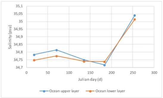
Figure 14 – Ocean boundaries salinity curves.
Salinity at the ocean border shows lower values in the winter and peak in spring. The maximum value is about 35 psu and the lower values about 34.7 psu, both in the ocean upper layer. The average salinity in the ocean is 34.8 psu.
Initial salinity values were defined for all boxes, with the absent of a determined value for day 1 (the 1th of January) the value for the 18th was used. This value was determined using the same methods as for temperature. Table 3 shows the determined values for each box.
Table 3 – Initial salinity conditions for each box.
Box Box 1 Box 2 Box 3/4 Box 5 Box 6 Box 7/8
Salinity (psu)
34.79 34.86 34.80 34.74 34.78 34.76
2.7
State variables
Pelagic state variables are forced at the ocean boundary. This means that there is an independent annual flux for each variable coming from the ocean, and the rest is dependent on mixture, transport, consume or new inputs.
The nutrients object contains 5 state variables: ammonia; nitrite; nitrate; phosphate; and silica; All of these state variables are forced in the ocean layer.
The phytoplankton object uses: the phytoplankton biomass; and others not analysed. The phytoplankton biomass growth is dependent on light, nutrients, exudation, respiration (light and dark), natural mortality, and removal by other organisms such as filter-feeding shellfish.
34,7 34,75 34,8 34,85 34,9 34,95 35 35,05 35,1
0 50 100 150 200 250 300
Sa li n it y ( p s u )
Julian day (d)
28 Suspension matter object has 2 state variables: suspension matter; and particulate organic matter; both are forced in the ocean layer, and are affected (inside each box) by phytoplankton mortality, deposition processes, and mineralization.
2.8
Nutrients
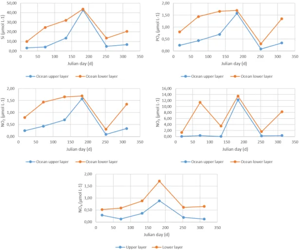
This object was processed similarly to the remaining to the following variables: ammonia, nitrite, nitrate, phosphate, and silica. The only difference was that the only data available for these nutrients was for station 1 (the one further from the ocean boundary). Figure 15 describe the boundary conditions for each nutrient.
Figure 15 – Boundary conditions for silica, phosphate, nitrite, nitrate and ammonia.
29
Table 4 – Initial conditions for each box
Box 1 Box 2 Box 3 Box 4 Box 5 Box 6 Box 7 Box 8
NH2
(µmol L-1)
0.01 0.01 0.01 0.01 0.10 0.10 0.10 0.10
NH3
(µmol L-1)
0.07 0.07 0.07 0.07 1.35 1.35 1.35 1.35
NH4
(µmol L-1)
0.28 0.28 0.28 0.28 0.52 0.52 0.52 0.52
Si
(µmol L-1)
3.27 3.27 3.27 3.27 9.80 9.80 9.80 9.80
PO4
(µmol L-1)
0.24 0.24 0.24 0.24 0.80 0.80 0.80 0.80
2.9
Suspended Matter
A series of data collected by Probyn (unpublished) - station positions described in Monteiro and Largier, (1999) was used to determine suspended particulate matter (SPM) and particulate organic matter (POM). These data set came with SPM and particulate organic carbon (POC). To determine particulate organic matter the following formula was used:
𝑃𝑂𝑀 = 𝑟 ∗ 𝑃𝑂𝐶
Being r = 1,88(Lam and Bishop, 2007). These data was only available for some days of February
and March, but for a series of areas in the Bay, as Figure 16 shows. For the ocean boundary
transect A was used. For the Big Bay initial values the Z values, for the Small Bay the Y values
30
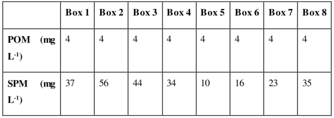
Table 5 – Initial conditions for each box to POM and SPM
The ocean boundary curves are described in the charts below. The model extrapolated the curve
for the rest of the year alone. Both SPM and POM have considerably higher concentrations in the upper layer.
Figure 16 – SPM (left side) and POM (right side) boundary conditions.
2.10
Phytoplankton
Phytoplankton boundary conditions curve (Figure 17) was drawn using the same methods as for Nutrients. The curve shows a peak around September.
Box 1 Box 2 Box 3 Box 4 Box 5 Box 6 Box 7 Box 8
POM (mg
L-1)
4 4 4 4 4 4 4 4
SPM (mg
L-1)
31
Figure 17 – Boundary phytoplankton biomass.
Using the available data the initial values for each box were calculated and inserted into the model. Table 6 shows the initial values calculated for each box.
Table 6 – Initial phytoplankton biomass for each box
Box number Box 1 Box 2 Box 3 Box 4 Box 5 Box 6 Box 7 Box 8
Phytoplankton
biomass
(µg chl a L-1)
8.6 2.3 5.5 5.5 3.9 2.1 11.0 11.0
2.11
Parameters
Standard parameterization from other models such as Belfast Lough model built by Ferreira et al., (2008), were used and adjusted in this model system where applicable. The parameters used to regulate phytoplankton are shown in the Table 7. “Pmax” and “Ks” are used in Michaelis Menten equation and regulate the Phytoplankton growth based on nutrient concentration. The following equation represents the Michaelis-Menten equation for phytoplankton growth; P is phytoplankton growth and [N] nutrient concentration.
𝑃 =𝑃𝑚𝑎𝑥 ∗ [𝑁]𝐾𝑠 + [𝑁]
“Iopt” is used in Steele, (1962) equation and is defined as the optimum light for phytoplankton production, above this value there is photo-inhibition, and the production decreases. This equation is described below, being “Ppot” the potential production and “I” the light energy:
0 5 10 15 20 25 30
0 50 100 150 200 250 300
P h y to p la n k to n b io m a s s ( µ g c h l a L -1) Time (d)
32
𝑃𝑝𝑜𝑡 =𝑃𝑚𝑎𝑥 ∗ 𝐼𝐼𝑜𝑝𝑡 ∗ 𝐸𝑥𝑝(1 −𝐼𝑜𝑝𝑡)𝐼
“Maintenance respiration” and “Respiration coefficient” are the energy consumed during the night and during production process respectively, used in the total budget equation.
Table 7 – Phytoplankton parameters used.
Parameter Value Description
Pmax (h-1) 0.3 Maximum phytoplankton production
Ks (µmol L-1) 2 Half saturation constant
Lopt (W m-2) 200 Optimum light intensity
Dead loss (d-1) 0.01 Percentage of dead loss per day
Maintenance respiration (d-1) 0.4 Energy spent during low production (night) Respiration coefficient (d-1) 0.3 Energy spending rate during production (day)
33
Table 8 – Suspended particle matter used parameters.
Parameter Value Description
SPM resuspension (d-1) 0.50 Resuspension ratio to SPM
Turbulence (d-1) 0.10 Turbulence ratio
POC fraction (no units) 0.16 SPM fraction of POC
POM mineralization rate (d-1) 0.060 POM mineralization rate
POM to nitrogen (DW to N) 0.046 POM to nitrogen in mineralization POM to phosphorus (DW to P) 0.0034 POM to phosphorus in mineralization
2.12
Shellfish
Winshell was used to test the growth potential of the two bivalve species in both boxes, using temperature, SPM, POM, salinity, and phytoplankton results from the model. These values were only used for calibration, and do not consider competition, as the growth is considered individually.
In order to simulate the reality in Saldanha at the moment, several farmers were contacted for information about their culture practices, location, areas under production, and production values. Small Bay shelters the production of both mussel and oyster, as Big Bay only for oysters. The farms are located only in the upper boxes, namely boxes 3 and 4.
34
Table 9 – Companies working in Saldanha Bay, respective annual production and licensed area.
Company Product Location Area
(ha)
Annual production
(ton)
Oyster Saldanha Bay Oyster Company
Small Bay and Big Bay
35
(10 SB + 25 BB) 525
West Coast Big Bay 5 140
Blue Safire Pearls
Small Bay 5 40
Total - - 45 705
Mussel Imbaza Mussels Small Bay 30 1000
Blue Ocean Mussels
Small Bay 50 1000
Total - - 80 2000
35
Table 10 – Mussel and oyster production, number of seeds, farm area, seed and harvested shellfish weight.
Shellfish Parameters Box 3 (Big
Bay)
Box 4 (Small
Bay)
Mussel Farm area (ha) - 80
Number of seeds - 50 million
Seed weight (g) - 0,65 g
Harvested weight (g) - 25 – 40 g
Oyster Farm area (ha) 30 15
Number of seeds 5 million 2 million
Seed weight (g) 4.3 4,3 g
37
3
Results and Discussion
3.1
Water temperature
Temperature in the Outer Bay is lower than in the remaining boxes, as it is more strongly under the effect of the ocean circulation water. In the Outer Bay the temperature ranges between 11 ºC and 15 ºC. The Big and Small Bay have a maximum of 18 ºC and a minimum 11 ºC. Langebaan
has the higher temperatures with a maximum of 20 ºC.
Figure 18 show’s temperature stratification during the summer period in all boxes except for
boxes 2 and 6, which is in agreement to what has been studied in Monteiro and Largier, (1999).
Water temperature in the upper boxes is higher during the summer, lower boxes show higher values during the winter due to the break of the thermocline. Langebaan Lagoon has a more homogeneous water temperature depth profile (less stratification) as the remaining areas. As such,
both boxes 2 and 6 have warmer water during the summer and colder in the winter.
The general presence of thermocline during the summer and mixture in the winter in all areas is accordingly to the reality in the bay. The temperature range and the differences between boxes seem also very acceptable.
38
3.2
Salinity
Salinity shows an identical profile in all boxes, the lower values are observed in winter, minimum of 34.7 and a maximum value of 35 psu in the spring. The average salinity is 34.8 psu.
Figure 19 – Salinity results for each box.
Salinity data is available to boxes 1, 3, 5, and 7, therefore, and as all boxes have very similar results respecting salinity, only this boxes were tested. All boxes correlated strongly (r>0.945; v=3) except box 3 (r=0.339; v=3). Even without correlation box 3 had identical mean salinity values (34.80 psu against 34.78 measured) and showed a lower value during winter as measured value, as the remaining boxes did. As a result all boxes seem to have acceptable salinity results.
3.3
Dissolved Inorganic Matter
The nutrient variable used for the phytoplankton growth is dissolved inorganic carbon (DIN), the sum of NO2, NO3, and NO4, as such, these nutrients are analysed as DIN. The results obtained, show a similar profile for all boxes, all boxes have a major peak in the winter with two smaller peaks during summer. The average DIN is 4 µmol L-1, the maximum is 14 µmol L-1 and the minimum value is close to 0 µmol L-1. Figure 20 illustrates DIN annual variation.
34,7 34,75 34,8 34,85 34,9 34,95 35 35,05
350 400 450 500 550 600 650 700
Sa
li
n
it
y
(
p
s
u
)
Julian day (d)
39
Figure 20 – DIN results for each box.
The only data available to test the nutrient results is the same used to insert them, and therefore in station 1. Most boxes had average annual DIN close to the data used to build the model, except for box 2 which had lower values. Table 11 illustrates the annual average DIN measured and modelled for the different boxes.
Table 11 – Comparison between measured average DIN and mean DIN results for each box.
Box 1 Box 2 Box 3 Box 4 Upper layer Box 5 Box 6 Box 7 Box 8 Lower layer
DIN
(µg L-1)
3.4 0.75 2.63 2.22 2.6 6.5 6.9 6.5 4.9 7.6
Boxes 2 and 6, as expected, have different values from the remaining, because they have a very distinct morphology and a weak connection to the remaining boxes. The observed DIN mean value for each box is not too distant from the measured ones and the spatial variability within the Bay is not known, so this shows only that this values are inside an acceptable range.
DIN may vary substantially and it is difficult to predict, due to the dynamics and communication with the other objects, namely, phytoplankton and POM. These dynamics alter DIN in the water column, which is consumed by phytoplankton and augmented by POM mineralization.
0 2 4 6 8 10 12 14 16
360 410 460 510 560 610 660 710 760
DI
N
(
u
m
o
l
L
-1)
Julian day (d)
40
3.4
Phosphate
As observed in figure 21, the 8 boxes have a similar curve for the phosphate concentration. The curve has three peaks: a maximum value in June; an intermediate peak in the autumn; and a smaller one in the spring.
Figure 21 – Phosphate annual results for each box.
The tests made to phosphate are similar to the ones made to DIN (same data source). All upper boxes correlate with measured data (r>0.958; v=4) and none of lower boxes correlates, (r<0.811; v=4). The upper boxes show higher values than the measured ones, about 2 times the measured values. The lower boxes have very similar values to the measured ones. It is difficult to conclude anything besides the average phosphate concentration results are in an acceptable range of values.
Table 12 – Measured average phosphate comparison with mean results phosphate for each box.
Box 1 Box 2 Box 3 Box 4 Upper layer Box 5 Box 6 Box 7 Box 8 Lower layer PO4
(µg L-1) 0.84 1.0 1.0 1.0 0.56 1.0 1.1 1.1 1.1 1.2
0 0,2 0,4 0,6 0,8 1 1,2 1,4 1,6 1,8
360 410 460 510 560 610 660 710 760
P h o s p h a te ( µ g L -1)
Julian day (d)
41
3.5
Suspended Particulate Matter
The SPM shows a relatively stable evolution across the year, with 4 small peaks occurring approximately every 3 months. The maximum value is 32 mg L-1 the minimum 21 mg L-1 and the average 26 mg L-1.
Figure 22 – SPM results for each box.
The only SPM data available is for a 10 day period, which is not sufficient to test SPM. Therefore there can only be commented that SPM results are inside the data range, as the measured range is: 9 to 61 mg L-1 and the results range is 21 to 32 mg L-1, which is acceptable.
19 21 23 25 27 29 31 33
350 400 450 500 550 600 650 700
SP
M
(
m
g
L
-1)
Julian day (d)