BJRS
RADIATION SCIENCES
07-03B (2019) 01-14ISSN: 2319-0612 Accepted: 2019-06-14
Bayesian estimation of the relative deviations between
activities in the radionuclide standardization
Cacais
a,bF.L., Delgado
aJ.U., Loayza
bV.M., Rangel
aJ.A.
a Instituto de Radioproteção e Dosimetria – IRD/LNMRI, Rio de Janeiro- RJ, Brazil b Instituto Nacional de Metrologia, Qualidade e Tecnologia – Inmetro, Rio de Janeiro- RJ,
ABSTRACT
The dissemination of the activity is performed from radionuclide sources prepared in a sequence of dilutions and weighing methods. In this process, the activity of the source can be estimated statistically from the deposited mass and the activity concentration of the master solution. After preparation, the activity is obtained from absolute or relative measurement methods. However, the methods of activity determinations used may not fulfill the necessary independence of the conventional statistical approach due to the presence of possible correlations between activities that arise with the use of the same standardized sources or with the same method of quantity measurements. In this paper, Bayesian estimates for the relative deviation of activities and their uncertainty were obtained in order to evaluate the performance of the main sources’ preparation method. The estimate result (0.55 ± 0.27) % for a data set of radionuclide standardization performed between 2017 and 2018 at LNMRI, although close to zero, shows one should investigate possible effects affecting the preparation and measurement of the sources. This Bayesian estimate was validated by monte carlo simulation method.
1.
INTRODUCTION
In the area of Radionuclide Metrology, the dissemination of activity [1] is carried out from radionuclide sources (standards for the dissemination of quantity) prepared from a sequence of dilutions and weighing [2] of a solution with high concentration of activity. Dilutions are carried out in glass ampoules with a stable isotope acid carrier solution of the radionuclide in order to maintain the stability of the standard and avoid the adsorption of radionuclides on the inner wall of the flask and heavy [3]. Weighing are performed by means of the several differential weighing methods (the pycnometer method, the substitution method, elimination method and modified elimination method), depends on the required uncertainty associated to activity per mass of the source [4]. After the source preparation, the activity is determined from absolute or relative measurement methods for liquid or solid sources [5].
In this process of preparation of sources, two estimates of activity are available, the first obtained from the multiplication of the mass deposited by the activity concentration of the master solution and the second one obtained from the measurement methods. As the activity measurement does not change the activity of the prepared source, the relative deviation between the two activity values can be used to evaluate the performance of the process of preparation of sources and possible effects between the preparation of solid and liquid sources and the measurement of the activity. In order to performing these evaluations in presence of set of relative deviation and its uncertainty a mean value that summarizes all information about deviation is required.
The problem to estimation of the mean value should be faced as that of the estimation of the key-comparison reference value (KCRV) for a data set. By this way a mean value for the relative deviation as the weighted mean based on classical statistical is recommended [6]. However, the presence of correlations between the relative deviation arisen from usage of the same standard sources and the activity measurement method does not comply with the independence required to this statistical approach. Thus, in order to get around this problem, in this work, a Bayesian estimate for the weighted mean of the relative deviation was determined for a data set of 45 radionuclide standardizations performed between 2017 and 2018 at LNMRI.
2.
THEORETICAL BACKGROUND
2.1. Bayesian theory applied to relative deviation
The relative deviation of the activities is defined according to equation (1). In this work we consider the activity determined from the source preparation process Ad with uncertainty from the master solution, the measured activity of the radionuclide source A and its measurement uncertainty and, only as reference (without uncertainty) for the relative deviation, the average activity Am.
D = 𝐴𝐴 − 𝐴𝐴𝐴𝐴 𝑑𝑑
𝑚𝑚 (1)
The uncertainty of the relative deviation D is determined from the uncertainties of the activities A and Ad, all of activities were corrected to the same reference date.
The system of measurements of sources activities yields as results the activity A and associated uncertainty u, which are assumed to be based on a large number of counts after all corrections for systematic effects have been applied. It is considered that these results, when determined from the GUM [7], come from a normal probability distribution centered on ξ, which describes the measurement system, this is the likelihood function related to the parameter ξ, according (2) [8]. The same hypothesis is assumed for the activity determined after the preparation of the sources, Ad.
p(A, u|ξ) ∝ exp �− 12 �𝐴𝐴 − ξu �2� (2)
As the relative deviation defined in (1) is a function of the difference between the measured activity and the determined activity, its measurement system also obeys a normal distribution and thus, by changes of variables in (2), the likelihood function can be rewritten as a function of the relative deviation D, the measurement uncertainty of the relative deviation uD and the parameter η, as previously, the likelihood can be associated to a normal distribution, now centered on η, (3).
p(D, uD|η) ∝ exp �− 12 �𝐷𝐷 − η
uD �
2
� (3)
To determine the posterior probability distribution p (η | D, uD) it is necessary to define the a priori distribution p (η) associated to the parameter [9]. As we do not have any information about the behavior of the parameter η that allows us to associate some probability distribution to it, it is
natural to use a reference non-informative prior (4), that is a constant when the estimation is based on a location parameter [10].
p(η) ∝ 1 (4)
Thus, after the first measurement of activity A1 and uncertainty u1, the values D1 and uD1 are determined from (1). The posterior distribution p (η | D, uD) can be obtained (5).
p(η|D1, uD1) ∝ exp �− 12 �𝐷𝐷1u− η D1 �
2
� (5)
After observing the measurements sequences, conditionally independent given the parameter η,
D = {D1, .., Dn} and uD = {uD1, .., uDn}, the posterior distribution becomes (6).
p(η|𝐃𝐃, 𝐮𝐮D) ∝ exp �− 12 ��𝐷𝐷𝑖𝑖u− η Di � 2 𝑛𝑛 𝑖𝑖=1 � (6)
The exponent of the à posteriori distribution can be rewritten in order to represent it as a normal distribution. − 12 ��𝐷𝐷𝑖𝑖u− η Di � 2 𝑛𝑛 𝑖𝑖=1 = − 12 ��𝐷𝐷𝑖𝑖2 𝑢𝑢𝐷𝐷𝑖𝑖2 𝑛𝑛 𝑖𝑖=1 − 2η � 𝐷𝐷𝑖𝑖 𝑢𝑢𝐷𝐷𝑖𝑖2 𝑛𝑛 𝑖𝑖=1 + η2� 1 𝑢𝑢𝐷𝐷𝑖𝑖2 𝑛𝑛 𝑖𝑖=1 � (7)
The first term in (7) does not depend on the parameter η and only has known values, so it can be included in the normalization factor of the à posteriori (8).
p(η|𝐃𝐃, 𝐮𝐮D) ∝ exp �− 12 �𝑢𝑢𝑝𝑝12�η2− 2η𝑢𝑢𝑝𝑝2𝑏𝑏��� ∴ 1 𝑢𝑢𝑝𝑝2 ≡ � 1 𝑢𝑢𝐷𝐷𝑖𝑖2 𝑛𝑛 𝑖𝑖=1 ; 𝑏𝑏 ≡ �𝑢𝑢𝐷𝐷𝑖𝑖 𝐷𝐷𝑖𝑖 2 𝑛𝑛 𝑖𝑖=1 (8) In (8), the square of the term between brackets is completed by adding and subtracting (bu2p)2, where the last term in does not depend on the parameter η, so it can be included in the normalization factor. Then, the expression for à posteriori becomes (9).
p(η|𝐃𝐃, 𝐮𝐮D) ∝ exp �− 12 �𝑢𝑢1
𝑝𝑝2�η − 𝑏𝑏𝑢𝑢𝑝𝑝
2�2�� (9)
This expression for à posteriori distribution is the same of a random variable obeying a normal distribution with mean bu2p and variance u2p. Thus, from the definitions of b and u2p, it can be concluded that the expected value and the parameter variance are, respectively, the weighted mean and variance obtained from the measured values, which pertain to the sequences D and uD (10).
E(η|𝐃𝐃, 𝐮𝐮D) = 𝑢𝑢𝑝𝑝2 � 𝐷𝐷𝑖𝑖 𝑢𝑢𝐷𝐷𝑖𝑖2 𝑛𝑛 𝑖𝑖=1 e V(η|𝐃𝐃, 𝐮𝐮D) = 𝑢𝑢𝑝𝑝2 = �� 1 𝑢𝑢𝐷𝐷𝑖𝑖2 𝑛𝑛 𝑖𝑖=1 � −1 (10) In presence of previous knowledge about the correlation between each relative deviation Di, the presented theoretical description should be rewritten in matrix form. In such case, the probability distribution associated to the vector of deviations D* is a multivariate normal distribution with a
covariance matrix W, equation (11), where 1 is a unitary column vector and the superscript refers to
transpose vector [11].
p(𝐃𝐃∗, 𝐖𝐖|η) ∝ exp �− 1
2(𝐃𝐃∗− 𝟏𝟏η)𝐓𝐓𝐖𝐖−𝟏𝟏(𝐃𝐃∗− 𝟏𝟏η)� (11)
Due to the lack of conditional independence, the likelihood factorization in equation (6) is not possible. However the Bayes theorem and the consideration about a reference non-informative prior remains valid (12).
p(η|𝐃𝐃∗, 𝐖𝐖) ∝ exp �− 1
2(𝐃𝐃∗− 𝟏𝟏η)𝐓𝐓𝐖𝐖−𝟏𝟏(𝐃𝐃∗− 𝟏𝟏η)� (12)
As before, bracketed terms can be rearranged from a few multiplications and keep only the factors that contain the parameter (13).
p(η|𝐃𝐃∗, 𝐖𝐖) ∝ exp �− 1
2 �(𝟏𝟏𝑻𝑻𝐖𝐖−𝟏𝟏1) �η2− 2η �
𝟏𝟏𝑻𝑻𝐖𝐖−𝟏𝟏𝐃𝐃∗
𝟏𝟏𝑻𝑻𝐖𝐖−𝟏𝟏1 ���� (13)
A normal distribution for η can be obtained in analogy to the procedure used to obtain equations (8) and (9) (14). p(η|𝐃𝐃∗, 𝐖𝐖) ∝ exp �− 1 2 �(𝟏𝟏𝑻𝑻𝐖𝐖−𝟏𝟏1) �η − � 𝟏𝟏𝑻𝑻𝐖𝐖−𝟏𝟏𝐃𝐃∗ 𝟏𝟏𝑻𝑻𝐖𝐖−𝟏𝟏1 � 2 ��� (14)
The expected posterior value and variance are obtained, as before, from the terms in the normal distribution (15) [12].
E(η|𝐃𝐃∗, 𝐖𝐖) = 𝟏𝟏𝑻𝑻𝐖𝐖−𝟏𝟏𝐃𝐃∗
𝟏𝟏𝑻𝑻𝐖𝐖−𝟏𝟏1 e V(η|𝐃𝐃∗, 𝐖𝐖) = 1
𝟏𝟏𝑻𝑻𝐖𝐖−𝟏𝟏1 (15)
A coverage interval can be established from probability distribution, the same way as in classical statistics, by converting the normal distribution into a standardized normal distribution
Φ(z) and by defining a random variable Z as a function of the mean and standard deviation of à posteriori (16).
Z = [η − E(η|𝐃𝐃∗, 𝐖𝐖)] �V(η|𝐃𝐃⁄ ∗, 𝐖𝐖) (16)
Assuming two quantiles of the reduced normal -zγ and zβ that contain a coverage probability (1 − α), the probability of finding Z in the coverage interval [-zγ, zβ], which is given by equation (17).
P �−zγ ≤ [η − E(η|𝐃𝐃∗, 𝐖𝐖)] �V(η|𝐃𝐃⁄ ∗, 𝐖𝐖)≤ zβ� = Φ�zβ� − Φ�−zγ� = 1 − α (17) The interval covered with the quantiles (13) has length of (zβ−zγ)�V(η|𝐃𝐃, 𝐖𝐖), (18).
E(η|𝐃𝐃∗, 𝐖𝐖) − zγ �V(η|𝐃𝐃∗, 𝐖𝐖) ≤ η ≤ E(η|𝐃𝐃∗, 𝐖𝐖) + zβ �V(η|𝐃𝐃∗, 𝐖𝐖) (18) It is important to highlights that in Bayesian statistics the coverage interval, also called the credibility interval, is determined for the random variable, the parameter η, and the interval is deterministic [11], unlike in the classical statistics, where the coverage interval is given for the deterministic parameter and the interval is a random variable [13].
From the definition and symmetry of the reduced normal distribution, the probabilities of the quantiles, respectively, β and γ are related to the coverage probability, (19).
Φ�zβ� − Φ�−zγ� = 1 − (β + γ) = 1 − α ⇒ α = β + γ (19)
According to the range probability value (1 − α), several quantum zγ and zβ can be established for different probabilities β and γ; however, in Bayesian theory the confidence interval for the parameter is determined by the pair of quantiles that form the shortest length (zβ−zγ)�V(η|𝐃𝐃, 𝐖𝐖), subject to restriction (19). This minimum length interval may be different from the probabilistically symmetric range (usually used in classical statistics) for asymmetric or multimodal (multiple peaks) probability distributions. However, this is not the case for the normal distribution and other symmetric and unimodal distributions where the minimum and probabilistically symmetric length confidence intervals coincide, and β = γ = α / 2, (20).
E(η|𝐃𝐃∗, 𝐖𝐖) − zα 2
� �V(η|𝐃𝐃∗, 𝐖𝐖) ≤ η ≤ E(η|𝐃𝐃∗, 𝐖𝐖) + zα�2 �V(η|𝐃𝐃∗, 𝐖𝐖) (20) In this paper, the expanded uncertainty U that forms the confidence interval for the parameter η is defined, for a 95% coverage probability, by (21).
𝑈𝑈 = z2,5% �V(η|𝐃𝐃∗, 𝐖𝐖) (21)
3.
CALCULATION PROCEDURE
3.1. Input data
The data set obtained from 45 sources prepared between 2017 and 2018 are shown in Tables 1 and 2. In these Tables, the expanded uncertainty U is a relative one. The terms GMX, CI and AC refers to respectively gamma spectrometry, ionizing chamber and 4πβ-γ anti-coincidence counting methods. In standard ID column are indicated the ionizing chamber calibration factor (different for each nuclide) or the standard code. Solid (S) and Liquid (L) are the physical states of the source.
The covariance matrix W required in equation (15) was obtained from covariance matrix ψA between pairs of measurement activities, from covariance between pairs of estimated activities ψAd and the crossed covariance between measurement and estimated activities ψAd,A (22).
𝐖𝐖 = 𝐌𝐌−𝟏𝟏�Ψ
A+ ΨAd− ΨA,Ad− ΨA,AdT �𝐌𝐌−𝟏𝟏 (22)
In equation (22) the diagonal matrix M is composed by the mean of the activities. The elements
of each covariance matrix were calculated considering the square of the lowest standard uncertainty between equal radionuclides, measured with the same measurement method and radionuclide standard. This approach is justified because this kind of covariance is related to B-type uncertainties which should have the same value for the pairs of activities uncertainties.
Table 1.First 27data used to determine activity deviation and a posteriori parameters.
Master Solution Source
Radionuclide (kBq) Ad (%) U Method Stand. ID (kBq) A (%) U Method Stand. ID Code
137Cs 20.7 0.92 GMX Factor 21.1 1.3 GMX 24S99 14S03 137Cs 20.7 0.98 GMX Factor 21.4 1.4 GMX 24S99 67S08 137Cs 228.9 0.73 GMX Factor 221.3 1.4 GMX 24S99 74S14 137Cs 57.1 0.74 GMX Factor 60.0 1.3 GMX 24S99 193S14 137Cs 57.6 0.74 GMX Factor 56.7 1.4 GMX 24S99 214S14 241Am 0.106 1.4 GMX 32 0.11 9.2 GMX 32 14L17 152Eu 49.9 1.5 CI3 Factor 48.9 3.5 GMX 36 45L17 241Am 0.69 1.4 GMX 32 0.69 1.5 GMX 32 55L17 60Co 0.64 0.84 GMX 67 0.63 1.0 GMX 47 55L17 137Cs 1.02 2.7 GMX 113 1.04 2.8 GMX 79 55L17 210PB 1.06 2.5 GMX 17 1.00 3.5 GMX 8 55L17 57Co 1.06 0.76 CI3 Factor 1.08 1.7 GMX 35 55L17 133Ba 1.41 1.0 GMX 24 1.49 1.3 GMX 24 55L17 134Cs 1.66 0.85 CI3 Factor 1.71 2.8 GMX 60 55L17 54Mn 1.85 1.2 CI3 Factor 1.77 1.3 GMX 43 55L17 65Zn 2.12 1.8 CI3 Factor 2.33 2.0 GMX 36 55L17 226Ra 1.11 2.6 GMX 03 1.10 2.5 GMX 47 66L17 60Co 21.7 0.50 CI3 Factor 21.7 2.5 GMX 47 87L17 137Cs 11.3 1.3 CI3 Factor 11.4 2.8 GMX 79 88L17
60Co 20.8 0.50 CI3 Factor 21.0 1.2 CI3 Factor 87L17
241Am 6.2 1.4 GMX 32 5.8 1.3 GMX 52 18L18
241Am 5.8 1.4 GMX 32 5.5 1.4 GMX 52 17L18
60Co 2.48 1.3 NaI 10 2.47 1.3 NaI 107 47
60Co 2.48 1.3 NaI 10 2.5 6.2 CI3 Factor 47
226Ra 0.132 2.6 GMX 03 0.134 2.6 GMX 47 29L18
22Na 365 0.69 CI3 Factor 337 2.2 GMX 132S08 13S17
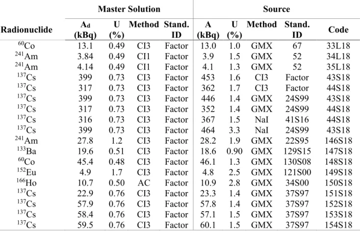
Table 2.Last 18data used to determine activity deviation and a posteriori parameters.
Master Solution Source
Radionuclide (kBq) Ad (%) U Method Stand. ID (kBq) A (%) U Method Stand. ID Code
60Co 13.1 0.49 CI3 Factor 13.0 1.0 GMX 67 33L18
241Am 3.84 0.49 CI1 Factor 3.9 1.5 GMX 52 34L18
241Am 4.14 0.49 CI1 Factor 4.1 1.3 GMX 52 35L18
137Cs 399 0.73 CI3 Factor 453 1.6 CI3 Factor 43S18
137Cs 317 0.73 CI3 Factor 362 1.7 CI3 Factor 44S18
137Cs 399 0.73 CI3 Factor 446 1.4 GMX 24S99 43S18
137Cs 317 0.73 CI3 Factor 352 1.4 GMX 24S99 44S18
137Cs 316 0.73 CI3 Factor 367 1.5 NaI 41S16 44S18
137Cs 399 0.73 CI3 Factor 464 3.3 NaI 24S99 43S18
241Am 27.8 1.2 CI3 Factor 28.2 1.9 GMX 22S95 146S18 133Ba 19.6 0.51 CI3 Factor 18.6 0.90 GMX 129S15 147S18 60Co 45.4 0.48 CI3 Factor 46.1 1.3 GMX 130S08 148S18 152Eu 4.9 1.7 CI3 Factor 4.8 2.5 GMX 121S00 149S18 166Ho 10.7 0.50 AC Factor 10.9 2.8 GMX 34S00 150S18 137Cs 22.9 0.76 CI3 Factor 23.3 1.4 GMX 37S97 151S18 137Cs 57.9 0.76 CI3 Factor 57.8 1.4 GMX 37S97 152S18 137Cs 58.4 0.76 CI3 Factor 57.1 1.5 GMX 37S97 153S18 137Cs 59.5 0.76 CI3 Factor 60.1 1.5 GMX 37S97 154S18
3.2. Validation by Monte Carlo method
The introduced theory was validated by the propagation of distributions principle as stated in JCGM 101 [8]. It was performed 7 × 10⁵ simulations for each random variable normally distributed A and Ad in Table 1. The mean of the normal distribution is the activity while the standard deviation is considered the relative standard uncertainty. The covariance matrix W also took part in
this simulation which was implemented by Monte Carlo method (MCM) using a properly spreadsheet plugin.
4.
RESULTS AND DISCUSSION
Table 2 shows the expected value and the expanded uncertainty for the parameter η of the posterior distribution of the relative deviation D obtained by Bayesian theory and Monte Carlo method. These results are very compatible so one can consider the theory is validated.
Table 2.A posteriori estimates for parameter η .
E[η|D,uD]
(%) (%) U
Bayesian 0.5514 0.27
MCM 0.5512 0.26
Figure 1: MCM results for parameter η.
Figure 1 shows the simulation results by MCM which confirms the normal distribution for the parameter η. Besides, the parameters kurtosis and skewness emphasizes the convergence for a normal distribution to the simulation of the experimental data.
Figure 2 shows the comparison between the estimated values and the values of the individual relative deviations Di for the radionuclide sources.
Figure 2: Individual relative deviations Di, expected posterior value E[η | D, uD] and confidence interval limits for parameter η.
It is important to note that if the covariance was not considered the expected value would be almost the double 1.16% with the same uncertainty so it would affected by the greater values which are responsible for the dispersion between the individual deviations. It can clearly observed with respect to the set of 137Cs sources at right upper corner.
5.
CONCLUSIONS
From the radioactive decay law, it is expected that a source of radionuclides will naturally reduce activity, and that with the application of corrections to these effects, as was done in this paper, the variation of the activity with time is zero. However, the result (of this work) indicates that the variation of the activity between the preparation of the sources and the measurement is positive, although it is very close to zero, but should be of order 1% if the lack of independence was not considered. This result may be a consequence of effects on source preparations, such as residual evaporation and correction of the balance indication, or effects arising on activity measurements resulting, for example, from calibration factors. A further research will be done to test these hypotheses and adequately conclude on the cause of the positive relative deviation between activities.
One can conclude as a performance characteristic to preparing process that the accuracy to prepared sources from a nominal activity value previously specified is not better than (0.55 ± 0.27) %.
ACKNOWLEDGMENT
Scholarship program PRONAMETRO / Inmetro.
REFERENCES
[1] CHRISTMAS, P. Traceability in radionuclide metrology. Nucl. Instrum. Methods Physics. Res. vol. 223, p. 427–434, 1984.
[2] CACAIS, F, et al. Validação da incerteza de pesagens no preparo de padrões de radionuclídeos
por método de monte carlo, CBMRI, 2016. Available at: <
http://media.2018.cbmri.org.br/media/uploads/s/[email protected]_1537223354_318198.pdf > Last accessed: 19 Feb. 2019.
[3] SIBBENS, G.; ALTZITZOGLOU, T. Preparation of radioactive sources for radionuclide metrology. Metrologia, vol. 44, p. S71–S78, 2007.
[4] LOURENÇO, V.; BOBIN, C. Weighing uncertainties in quantitative source preparation for radionuclide metrology. Metrologia, vol. 52, p. S18–S29, 2015.
[5] VERDEAU, E. Metrological references for nuclear measurements provided by LNE-LNHB to users through a strict traceability chain, IEEE - 1st International Conference on Advancements in Nuclear Instrumentation, Measurement Methods and their Applications,
2009.
[6] COX, M. G. The evaluation of key comparison data. Metrologia, vol. 39, p. 589–595, 2002.
[7] JCGM, BIPM, IEC, IFCC, ILAC, ISO, IUPAC, IUPAP and OIML 2008 Guide to the
Expression of Uncertainty in Measurement (GUM:1995 with Minor Corrections) JCGM
100:2008 (Sèvres: Bureau International des Poids et Mesures).
[8] JCGM. Evaluation of Measurement Data—Supplement 1 to the ‘Guide to the Expression of Uncertainty in Measurement’—Propagation of Distributions using a Monte Carlo Method
[9] KOCH, K. Introduction to Bayesian Statistics, 2ª ed., Berlin, Springer, 2007.
[10] LIRA, I; KYRIAZIS, G. Bayesian inference from measurement information. Metrologia,
vol. 36, p. 163–169, 1999.
[11] MIGON, H. Statistical Inference: an Integrated Approach, 1ª ed., London, Oxford
University Press, 1999.
[12] WUBBELER, G., et al. Maintaining consensus for the redefined kilogram. 2018.
Available at: <
https://iopscience.iop.org/0026-1394/55/5/722/media/METaadb6b_Suppdata.pdf>. Last accessed: 19 Feb. 2019.


![Figure 2: Individual relative deviations D i , expected posterior value E[ η | D, u D ] and confidence interval limits for parameter η](https://thumb-eu.123doks.com/thumbv2/123dok_br/18277851.881294/11.892.90.811.239.774/individual-relative-deviations-expected-posterior-confidence-interval-parameter.webp)
