* Corresponding author: E-mail: [email protected]
Received: March 10, 2016 Approved: October 26, 2016
How to cite: Bagio B, Bertol I, Wolschick NH,
Schneiders D, Santos MAN. Water
erosion in different slope lengths
on bare soil. Rev Bras Cienc Solo. 2017;41:e0160132.
https://doi.org/10.1590/18069657rbcs20160132 Copyright: This is an open-access article distributed under the terms of the Creative Commons Attribution License, which permits unrestricted use, distribution, and reproduction in any medium, provided that the original author and source are credited.
Water Erosion in Different Slope
Lengths on Bare Soil
Bárbara Bagio(1)
, Ildegardis Bertol(2)*
, Neuro Hilton Wolschick(1)
, Danieli Schneiders(1) , and Maria Aparecida do Nascimento dos Santos(1)
(1)
Universidade do Estado de Santa Catarina, Departamento de Solos e Recursos Naturais, Programa de Pós-graduação em Ciência do Solo, Lages, Santa Catarina, Brasil.
(2)
Universidade do Estado de Santa Catarina, Departamento de Solos e Recursos Naturais, Lages, Santa Catarina, Brasil.
ABSTRACT: Water erosion degrades the soil and contaminates the environment, and one
influential factor on erosion is slope length. The aim of this study was to quantify losses of soil (SL) and water (WL) in a Humic Cambisol in a field experiment under natural rainfall conditions from July 4, 2014 to June 18, 2015 in individual events of 41 erosive rains in the Southern Plateau of Santa Catarina and to estimate soil losses through the USLE and RUSLE models. The treatments consisted of slope lengths of 11, 22, 33, and 44 m, with an average degree of slope of 8 %, on bare and uncropped soil that had been cultivated with corn prior to the study. At the end of the corn cycle, the stalk residue was removed from the surface, leaving the roots of the crop in the soil. Soil loss by water erosion is related linearly and positively to the increase in slope length in the span between 11 and 44 m. Soil losses were related to water losses and the Erosivity Index (EI30), while water losses were related to rain depth. Soil losses estimated by the USLE and RUSLE model showed lower values than the values observed experimentally in the field, especially the values estimated by the USLE. The values of factor L calculated for slope length of 11, 22, 33, and 44 m for the two versions (USLE and RUSLE) of the soil loss prediction model showed satisfactory results in relation to the values of soil losses observed.
Keywords: soil loss, water loss, USLE, RUSLE.
INTRODUCTION
Water erosion is the main factor of soil degradation since it impoverishes the place of origin of erosion and pollutes the environment outside of that place, especially water resources. Rainfall erosion is influenced by rainfall, soil, relief, soil cover, and management and conservation practices, including the stages of detachment, transport, and deposition that occur concomitantly (Ellison, 1947; Wischmeier and Smith, 1978; Renard et al., 1997). Rain is the active agent in rainfall erosion and the magnitude of its influence depends on its intensity, duration, and volume, which is reflected in erosivity. The soil is the passive agent and its susceptibility to erosion depends on its intrinsic characteristics, expressed by erodibility. In untilled soil, without surface cover and without conservation practices, soil erosion depends predominantly on erosivity, erodibility, and on the particular conditions of soil relief (Wischmeier and Smith, 1978; Renard et al., 1997).
The relief factor is represented by the length, the degree of slope, and the shape of the slope, with remarkable influence on water erosion, since it is an energy factor that maximizes surface runoff. The effect of slope length on erosion occurs through an increase in the volume and the speed of runoff, resulting in increased capacity of the runoff to disaggregate and transport sediments (Bagarello and Ferro, 2010).
The effect of slope length on SL is not yet sufficiently understood. Research results on this topic are different and even contradictory since intrinsic characteristics of the soil, type of use, cropping system, and management of soil and crops influence this relation (Lal, 1988). Zingg (1940) observed a three-fold increase in SL upon doubling slope length, whereas Laflen and Saveson (1970) demonstrated that SL increased linearly with increasing length. Bertoni et al. (1972) noted an increase in SL of around 1.5 times upon doubling slope length, a ratio also observed by Wischmeier and Smith (1978). According to Rejman et al. (1999), SL decreased with increasing slope length, whereas Silva and De Maria (2011) observed practically insignificant SL in slope lengths of 25, 50, and 75 m. They could not, therefore, establish a relation between these two variables. These studies were carried out under natural rainfall conditions on a plot scale in various locations and rainfall regimes, with different types of land use and soil management practices, different plants and crop residues, and variable steepness of terrain, which partially explains the diversity of the results. However, in general, in bare and uncovered soil, SL increased with length of slope.
Factors that influence erosion are represented and constitute the structure of the erosion prediction model in the USLE and RUSLE versions, widely used to predict average SL on an annual basis (Foster et al., 1977; Wischmeier and Smith, 1978), whose formula is as follows:
A = R K L S C P Eq. 1
in which A = average soil loss (Mg ha-1 yr-1); R = rainfall erosivity factor (MJ mm ha-1 h-1 yr-1); K = soil erodibility factor (Mg ha h ha-1 MJ-1 mm-1
); L = length of slope factor (dimensionless); S = degree of slope factor (dimensionless); C = soil cover and management factor (dimensionless); and P = practice of conservationist support factor (dimensionless).
In the USLE and RUSLE, the L factor is calculated according to the following general equation:
L = 22.1
(
λ)
mEq. 2 in which λ = slope of any length, m; 22.1 = standard slope length of the plot, m; and
and 0.2 for slope <0.01 m m-1) in the USLE. In the RUSLE, the exponent m is also dependent on the slope. It is obtained using the equation:
m =1 + ββ Eq. 3
in which β = ratio between erosion in the rill and erosion interrill. In soil conditions moderately susceptible both to erosion in rill and to erosion interrill, β is calculated by the following equation:
β =
(
0.0896)
senθ
[3(senθ)0.8 + 0.56] Eq. 4
in which θ = slope angle.
Modification of the model to the RUSLE version, with inclusion of the value of β for calculation of the m exponent, resulted in an increase in the predictive ability of the RUSLE in relation to the USLE, especially on slopes up to a length of approximately 100 m (Renard et al., 1997).
Based on the above, the following hypotheses were formulated: in bare soil, the relation between slope length and soil loss is linear; soil losses are related to water losses and the Erosivity Index (EI30), while water losses are related to the rain depth; soil losses are underestimated by the USLE and RUSLE compared to the values observed in the field; and the L factor of the USLE and modified L factor of the RUSLE result in a satisfactory estimate of soil loss.
The aim of this study was to quantify soil losses and water losses experimentally in the field, assess soil losses using the USLE and RUSLE models, and relate the soil loss values estimated by the USLE and RUSLE with the values observed in the field for different slope lengths.
MATERIALS AND METHODS
This study was conducted under natural rainfall conditions on a plot scale at 27° 49’ S and 50° 20’ W and 923 m altitude in Lages, Santa Catarina, Brazil. The weather is the Cfb type in the Köppen classification system according to Wrege et al. (2011), with erosive rainfall totaling 1,533 mm and annual erosivity totaling 5,033 MJ mm ha-1 h-1 (Schick et al., 2014a). The soil is classified as a Cambissolo Húmico Alumínico léptico (Santos et al., 2013), a Humic Cambisol, in according to the criteria of the IUSS/WRB (2006), with clayey texture and a siltstone substrate, whose erodibility is 0.0175 Mg ha h ha-1 MJ-1 mm-1 (Schick et al., 2014b).
In 2012 the ground was tilled a number of times with plow and harrow to incorporate 5 Mg ha-1 of dolomitic limestone and 300 kg ha-1 of formulated fertilizer 5-20-10 (N-P-K). In November, beans were sown manually and harvested in April 2013, followed by one plowing and one harrowing and then the soil remained fallow until July, at which time one more plowing and two harrowings were done. In November, corn was sown, without fertilizer, with the aid of a “saraquá” (manual seeder), and it was harvested in May 2014. Stalk residue was removed from the soil surface. Over these conditions, the plots that would define the treatments were set up.
Four treatments (T) were evaluated in two field replications, consisting of different slope lengths with varying degrees of slope, due to topographical variation of the ground, as follows: T1 - slope length of 11 m and average degree of slope of 0.084 m m-1; T2 - slope length of 22 m and an average degree of slope of 0.082 m m-1; T3 - slope length of 33 m and average degree of slope of 0.077 m m-1; and T4 - slope length of 44 m and average degree of slope of 0.076 m m-1. The soil was kept without cultivation and without plant cover during the study.
Collection of runoff in the field and processing of samples in the laboratory to calculate SL and WL were made according to Cogo (1978) from July 2014 to June 2015 in 41 erosive rainfalls.
The R factor for both versions of the model (USLE and RUSLE) was obtained by multiplication of total kinetic energy by the maximum intensity in 30 min, called the erosivity index (EI30). To obtain this index in daily rainfalls, erosive rainfalls were rated manually in segments of uniform intensity and recorded on spreadsheets. Subsequently, kinetic energy was calculated as reported by Wischmeier and Smith (1958), according to equation 5:
E = 0.119 + 0.0873 log I Eq. 5
in which E = kinetic unitary energy, MJ ha-1 mm-1; and I = rainfall intensity, mm h-1. This equation is applicable to rainfall intensities of up to 76 mm h-1. Above that threshold, the kinetic energy unit of the rainfall is considered constant at 0.2832 MJ ha-1 mm-1.
The soil K factor was calculated by the ratio between the value of the SL observed in the standard 22-m-length plot and the value of the R factor (EI30) of the rains in the experimental year for the USLE and RUSLE.
The values of the L factor for the USLE and RUSLE were calculated according to equation 2; the exponent m of equation 2 for the RUSLE was calculated according to equation 3, and the values of β in equation 3 were calculated according to equation 4.
The values of the C (soil cover and management) and P (conservation practice) factors were considered equal to one (1) since the soil was kept without cultivation and surface cover and no conservation practices were adopted in the year of the experiment. Due to variation in the degree of slope within each plot and among plots, we calculated the average S factor (degree of slope of the terrain factor) for each plot, as well as the S factor of the standard degree of slope of the USLE and RUSLE (0.09 m m-1), as proposed by Wischmeier and Smith (1978) and Renard et al. (1997).
For the USLE, the S factor was calculated using the following equation: S = 0.065 + 4.56 senθ + 65.41 (senθ)2
Eq. 6 in which S = steepness factor; and θ = slope angle.
To calculate the S factor of the RUSLE the following equation was used:
S = 10.8 senθ + 0.03 Eq. 7
For final adjustment of the SL values, a correction factor (Fc) was calculated based on the S factor calculated for the standard plot by equation 5, according to the following formula:
Fc = S 0.09 mm-1
Average S of the plot Eq. 8
The SL and WL data by water erosion were initially analyzed in regard to normality through the “Shapiro-Wilk” test and then subjected to analysis of variance; when the treatments differed, the average values were compared by the Tukey test (p≤0.05), using Assistat 7.7 Beta (Silva and Azevedo, 2016). Graphical relationships were made: soil loss (SL) × water loss (WL); SL × EI30; WL × rain depth (RD); L factor of the USLE × SL observed; L factor of the RUSLE × SL observed; SL estimated by the USLE × SL observed; SL estimated by the RUSLE × SL observed; and SL estimated by the USLE × SL estimated by the RUSLE.
RESULTS AND DISCUSSION
Losses of water and soil through erosion
The increase in water loss (WL) by surface runoff was linear with increasing rain depth (RD) (p≤0.01) (Figure 1a), as reported by Barbosa et al. (2012), Amaral et al. (2014), and Bertol et al. (2014). According to Bertol et al. (2014), the increase in RD results in an increase in the volume and speed of runoff and, therefore, in the erosive power.
There was an increase in SL values with an increased EI30 of the rains (p≤0.05) (Figure 1b), with greater dispersion of points than was seen in figure 1a. The points located above the linear regression line indicate that some rains with low EI30 values caused high SL values. The points below the line mentioned, show high EI30 rains that caused low SL. One of the reasons for this may be the water content in the soil prior to the rainfalls, a variable depending on the interval between rains. According with Istok and Boersma (1986), water content in the soil is a determining factor in the variation of water infiltration in the soil and, therefore, a factor in the variation of runoff and soil loss by erosion. Although the variation in water content in the soil has not been quantified, its effect in modifying SL can be more expressive than that of EI30 considering individual rainfalls, according to observations made by Eltz (1977). Furthermore, the observed dispersion can be explained by temporal variation in the rainfall pattern that determined its erosivity, as shown by the data of Schick et al. (2014b).
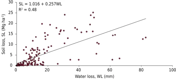
The erosive potential of rain (EI30) is associated with the shearing energy generated by runoff from the soil and the impact of raindrops (Wischmeier and Smith, 1958). In the condition of bare soil without cultivation, the absence of protection on the soil allows the erosive power of the rain to strengthen its capacity to produce erosion. Therefore, under the condition of bare and uncultivated soil, as was the case in this study, the WL explained the SL (p≤0.05) (Figure 2), which was more than could occur under conditions of cultivated soil covered by crop residue, as observed by Schick et al. (2016).
Figure 1. The relation between (a) values of water loss (WL) and rain height (RH) (p<0.01) and (b) values of soil losses (SL) and erosivity (EI30) (p<0.05) (individual values of each variable and
average of the treatments).
0 20 40 60 80 100
0 20 40 60 80 100
WL= - 6.042 + RH0.588 R2 = 0.70
Rain height, RH (mm)
Wa
ter loss, WL (mm)
0 200 400 600 800 1000
0 5 10 15 20 25
Erosivity, EI30 (MJ mm ha-1 h-1)
Soil loss, SL (Mg ha
-1)
SL = 1.579 + 0.019EI30 R2 = 0.33
On bare soil, the impact of raindrops acts on the surface, disaggregates the soil, facilitates formation of a surface seal during the rain and evolves into a crust, causing greater water loss through evaporation (Duley, 1939; Tackett and Pearson, 1965). Soil crusting was visually observed by the authors during the experimental period, but was not quantified. Several studies confirm the occurrence of sealing and crusting of the surface by the action of rain and/or runoff under various management conditions, especially on bare soil (Reichert et al., 1994; Reichert and Norton, 1995; Lado et al., 2004; Le Bissonnais et al., 2005; Rosa et al., 2013).
The SL per unit of area did not vary statistically among treatments (Table 1) showing only a tendency to increase with an increase in slope length, similar to results obtained by Bagarello and Ferro (2010) and in disagreement with Bertoni et al. (1972) and Wischmeier and Smith (1978). This tendency of increase can be observed in figure 3a. The theoretical line of adjustment indicates that in the length of 44 m of terrain, the SL increased 45.5 Mg ha-1 (regression coefficient = 1.455), in the average of the ramp.
Duplication of the slope length from 11 m to 22 m led to an increase of 9.2 % in SL in Mg ha-1 (Table 1), which was lower than the increase reported by Bertoni et al. (1972) and Wischmeier and Smith (1978). For those authors, upon doubling the length of the slope, soil losses are expected to increase an average of 50 %, ranging from 20 to 80 %. Furthermore, according to Wischmeier and Smith (1978), an increase in SL from the increase of slope length should result in a ratio, in which the value of the regression coefficient (b) ranges from 0.2 to 0.8, with an average of 0.5. The increase in erosion with the length of slope is explained by the greater erosive power of surface runoff, determined mainly by the increase in the volume and speed of runoff.
Table 1. Values of total soil losses in the different treatments obtained in the period from July 4, 2014 to June 18, 2015 and expressed in weight per unit of area and in weight for each slope length
studied (average of replications)
Treatment Soil loss
Mg ha-1
Mg
11 m 153 0.36 c
22 m 167 0.82 bc
33 m 183 1.32 b
44 m 201 1.93 a
CV (%) 18 12
Means values followed by different letters in the column differ statistically from each other by the Tukey test (p≤0.05).
Figure 2. Relation between soil losses (SL) and water losses (WL) (individual values of each variable and average of replicates) (p<0.05).
0 20 40 60 80 100
0 5 10 15 20 25 30
Water loss, WL (mm)
Soil loss, SL (Mg ha
-1)
Studies done before and after Wischmeier and Smith (1978) confirmed that there is a potential link between the increase in soil weight lost per unit of area and the increase in the length of the slope. By doubling the length of the slope, Zingg (1940) observed a threefold increase in total soil loss. Bertoni et al. (1972) found an increase of 1.4 and 1.6 times in SL when doubling the slope length from 25 to 50 m and from 50 to 100 m, respectively, with degree of slope between 6.5 and 7.5 % and average rainfall of 1,300 mm annually. In studies conducted in natural rainfall conditions on bare soil, Lal (1984) observed an increase in SL with an increase in slope length. Akeson and Singer (1984) reported that the SL ranged from 51 Mg ha-1 in a slope length of 2.4 m to 144 Mg ha-1 in a slope length of 14.7 m.
In other research studies under natural rainfall conditions, this tendency was not confirmed. With slope lengths of 0.25, 0.4, 1.0, 2.0, 5.0, 11, 22, 33, and 44 m in bare and uncultivated soil condition, Bagarello and Ferro (2010) observed that the SL did not vary with the length of the slope in 40 erosive rainfall events over 10 years. The explanation of these authors was that the increase in slope length had a moderate effect in increasing the erosion in the interrill and an appreciable effect on reduction of rill erosion. Thus, the relation found between the SL and the length of slope, plain and simple, under the conditions evaluated was not enough to explain the potential relation published by Wischmeier and Smith (1978). In studying slope lengths of 5, 10, and 20 m for four months, Rejman et al. (1999) found that the SL decreased with an increase in slope length.
Considering only the total weight of soil lost in each slope length studied (Table 1), the variation in SL was statistically significant among treatments (p≤0.05), from 0.36 Mg in the treatment with slope length of 11 m to 1.93 Mg in the treatment of 44 m. Doubling the slope length from 11 to 22 m increased SL 2.28 times, while doubling the length from 22 to 44 m increased the SL 2.35 times. This increase is confirmed in figure 3b. The theoretical line of adjustment indicates that at the length of 44 m of terrain, the SL increased 4.7 Mg (regression coefficient = 0.047) in the average of the ramp considering the eroded area in each treatment, i.e., 22 m2 in T1, 44 m2 in T2, 66 m2 in T3, and 88 m2 in T4.
The SL values observed in the field, calculated in terms of soil loss per unit of area (Mg ha-1 ) facilitated comparison with other studies in the literature. However, the loss per unit of area conceals the real differences between the treatments. Thus, it appears that in this study, this data should be presented as the total weight of soil lost in each length of slope.
The treatment of 22 m slope length (standard length for the USLE) exhibited SL of 167 Mg ha-1 (Table 1) under erosivity of 6,066 MJ mm ha-1 h-1
. Schick et al. (2014b), working with data from 20 years of an experiment in the same soil as this study, calculated SL Figure 3. Relation between soil losses (SL), weight × area (a) and weight (b) and slope lengths (SLe) (total values per treatment) (p<0.01).
0 10 20 30 40 50
140 150 170
160 180 190 200 210
WL = 136 + 1.455SLe R2 = 0.99
Slope length, SLe (m)
Soil loss, SL (Mg ha
-1)
0 10 20 30 40 50
0.0 0.4 0.8 1.6
1.2 2.0 2.4
Soil loss, SL (Mg)
SL = 0.195 + 0.047SLe R2 = 0.99
of 85.3 Mg ha-1 yr-1 under erosivity of 4.883 MJ mm ha-1 h-1, likewise for a treatment on a standard plot of the USLE. Therefore, the SL observed in 22 m of length was 2.18 times greater than the historical mean for the region obtained by these authors. This difference is explained as follows: in the study of Schick, the soil underwent conventional tillage (one plowing, two harrowings) twice a year; in addition, the erosivity that occurred between 2014 and 2015 was 20 % greater than the historical average. Moreover, since it was the first year of erosion assessment in this study, the soil had a large amount of sediment disaggregated by the treatments prior to setting up the study, facilitating transport by runoff, greater than the average erosion over 20 years obtained by Schick et al. (2014b). According to these authors, as soil erosion progresses over time, the SL decreases because the same erosive energy of the rain encounters a layer of soil more resistant to erosion.
Likewise under the soil conditions found in the standard plot of the USLE, Beutler et al. (2003) found SL of 71.16 Mg ha-1 yr-1 in a Latossolo Vermelho
(Oxisol) under erosivity of 11,005 MJ mm ha-1 h-1
, while Silva et al. (2009) obtained SL of 175 Mg ha-1 yr-1 in a Cambissolo Háplico (Inseptisol) with annual erosivity of 4,865 MJ mm ha-1 h-1. This demonstrates the wide variation in SL due to variations mainly from soil type and rainfall patterns.
The SL tolerance established for the soil used in this study was 9.6 Mg ha-1 yr-1 (Bertol and Almeida, 2000). The SL values for the treatments of 11, 22, 33, and 44 m were 16, 17, 19, and 20 times greater than that tolerance, respectively, demonstrating that bare soil should be avoided.
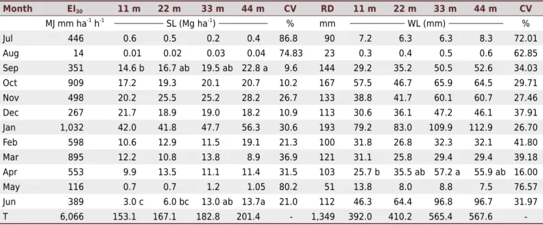
Soil loss exhibited wide numeric variation between months of the year and between treatments; it was 0.01 Mg ha-1 in August 2014 in the slope length of 11 m and 56.3 Mg ha-1 in January 2015 in the length of 44 m, according to the EI30, which ranged from 14 to 1032 MJ mm ha-1 h-1 among the respective months (Table 2).
In September and June, the SL showed a statistical difference (p≤0.05) among treatments. The WL ranged from 0.3 mm in August 2014 in the 11-m treatment to 112.9 mm in January 2015 in the 44-m treatment according to the RD that ranged from 23 to 193 mm between the respective months. There was a statistical difference (p≤0.05) in the WL only in April. Numerically, temporal variation of SL was 563 times for a variation of 74 times in EI30, while for WL, the temporal variation was 376 times for a variation of 8 times in the RD, demonstrating that the SL depended much more on the EI30 than the
Table 2. Values of erosivity (EI30), soil loss (SL), rain depth (RD), and water loss (WL) obtained from July 2014 to June 2015 and annual
total (T), in different treatments (average of replications)
Month EI30 11 m 22 m 33 m 44 m CV RD 11 m 22 m 33 m 44 m CV MJ mm ha-1
h-1
SL (Mg ha-1
) % mm WL (mm) %
Jul 446 0.6 0.5 0.2 0.4 86.8 90 7.2 6.3 6.3 8.3 72.01
Aug 14 0.01 0.02 0.03 0.04 74.83 23 0.3 0.4 0.5 0.6 62.85
Sep 351 14.6 b 16.7 ab 19.5 ab 22.8 a 9.6 144 29.2 35.2 50.5 52.6 34.03 Oct 909 17.2 19.3 20.1 20.7 10.2 167 57.5 46.7 65.9 64.5 29.71 Nov 498 20.2 25.5 25.2 28.2 26.7 133 38.8 41.7 60.1 60.7 27.46 Dec 267 21.7 18.9 19.0 18.2 10.9 113 30.6 36.1 47.2 46.1 37.91 Jan 1,032 42.0 41.8 47.7 56.3 30.6 193 79.2 83.0 109.9 112.9 26.70 Feb 598 10.6 12.9 11.5 19.1 21.3 100 31.8 26.8 32.3 32.1 41.80 Mar 895 12.2 10.8 13.8 8.9 36.9 121 31.1 25.8 29.4 29.4 39.18 Apr 553 9.9 13.5 11.1 11.4 31.5 103 25.7 b 35.5 ab 57.2 a 55.9 ab 16.00
May 116 0.7 0.7 1.2 1.05 80.2 51 13.8 8.0 8.8 7.5 76.57
Jun 389 3.0 c 6.0 bc 13.0 ab 13.7a 21.0 112 46.3 64.4 96.8 96.7 31.97 T 6,066 153.1 167.1 182.8 201.4 - 1,349 392.0 410.2 565.4 567.6
WL depended on the RD. This temporal variation in SL and WL was normal, due to the influence of climate on the characteristics of the rains, which determined their depth and erosivity, and to the temporal variability of water content in the soil, due to the interval between rains and to variation in climate. Lower variation of WL in comparison to SL is in accordance with what has been observed in studies on water erosion under various conditions (Schick et al., 2000; Beutler et al., 2003; Cogo et al., 2003; Schick et al., 2014) due to limits on water infiltration in the soil according to its characteristics.
The months of October 2014 and January 2015 concentrated 32 % of the annual EI30 and 27 % of the annual RD, and in those months, SL was equivalent to 19 % and WL to 16 % of the annual total, in the average of the treatments (Table 2). These values are similar to those reported by Schick (2014) and Schick et al. (2014b), who found that there is a close relationship between the SL and the EI30 and between the WL and the RD in bare soil conditions in an experiment at this same location. Thus, these two months are problematic in terms of soil and water conservation in the area of research because they concentrate most of the erosion due to the greater erosive potential of the rains on an annual basis.
The treatment in which the slope length was 11 m had WL equivalent to 29 % of the RD, considering the annual total, followed by 30 % in the treatment of 22 m, 42 % in that of 33 m, and 42 % in that of 44 m. Zingg (1940), in a compilation of data from various experiments conducted over 20 years with simulated rain, found that WL decreased with an increase in slope length, which was also verified by Lal (1983). A smaller increase in WL in longer slopes was observed by Silva and De Maria (2011). According to the author, the reduction in the rate of increase in water loss per unit of area can be explained due to greater possibility of water infiltration into the soil and/or evaporation on longer slopes, in which there is also greater variation of the degree of slope of the terrain compared to the shorter ones.
Estimation of soil loss through erosion by the USLE and RUSLE
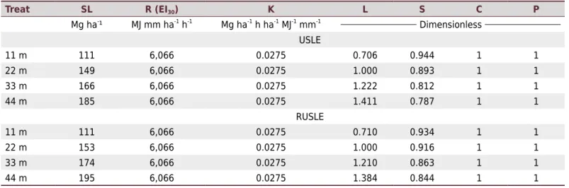
During the experimental period, total rainfall was 1,349 mm (Table 2), resulting from 41 erosive rains, with an absolute value of the EI30 index of 6,066 MJ mm ha-1 h-1 yr-1 (Tables 2 and 3). Schick et al. (2014a), studying the historical series of rainfall for 24 years for the same location, found an average annual number of erosive rainfalls of 51, 1,279 (mm) total rainfall, and EI30 index of 5,033 MJ mm ha-1 h-1 yr-1). Therefore, even with 20 % fewer erosive rains in this study than in the work of Schick, the depth and the EI30 of the rains were 5 and 21 % greater, respectively. The value of the K factor of 0.0275 Mg ha h ha-1 MJ-1 mm-1 calculated from data of the experimental year was 57 % greater than the value of 0.0175 Mg ha h ha-1 MJ-1 mm-1 found by Schick et al. (2014b) in a historical series of data over 20 years for the same soil.
Table 3. Values of SL estimated by the USLE and RUSLE, R factor (EI30), K factor, L factor, S factor, C factor, and P factor in the
different treatments (Treat) (average of replications)
Treat SL R (EI30) K L S C P
Mg ha
-¹ MJ mm ha-1 h-1
Mg ha-1 h ha-1
MJ-1 mm-1
Dimensionless USLE
11 m 111 6,066 0.0275 0.706 0.944 1 1
22 m 149 6,066 0.0275 1.000 0.893 1 1
33 m 166 6,066 0.0275 1.222 0.812 1 1
44 m 185 6,066 0.0275 1.411 0.787 1 1
RUSLE
11 m 111 6,066 0.0275 0.710 0.934 1 1
22 m 153 6,066 0.0275 1.000 0.916 1 1
33 m 174 6,066 0.0275 1.210 0.863 1 1
The values of the L factor calculated showed a lower numeric variation between the two versions (USLE and RUSLE) of the model, while the values of the S factor ranged more widely in the interval of the treatments (Table 3). For the USLE, the L factor ranged from 0.706 in the slope length of 11 m to 1,411 m in 44 m, whereas for the RUSLE, the same factor ranged from 0.710 to 1.384 in the respective slope lengths. For the S factor in the USLE, the range of values for these slope lengths was 0.944 to 0.787, whereas for the RUSLE, this variation was from 0.934 to 0.844.
The SL estimated by the USLE ranged from 111 mg ha-1 for the slope length of 11 m to 185 mg h1 for 44 m, whereas for the RUSLE, the variation in SL was from 111 to 195 mg h-1 in the respective treatments (Table 3). The USLE and RUSLE underestimated the SL compared to the observed values (Table 1) for the four treatments, despite the fact that the values of the R and K factors used in calculation of the SL estimated in the research period were higher than the values determined by Schick et al. (2014a,b). For the USLE, the estimate was 13 % lower than the observed data in the average of treatments, whereas for the RUSLE, the estimates were 10 % lower than those observed, with the error of the estimates decreasing with increasing slope length, for both versions.
The lower SL values predicted by the USLE and RUSLE in relation to the observed data occurred due to the fact that this model was developed for temperate climate conditions. There was thus an underestimation of the values of the model input factors, especially the R factor, due to discrepancy between the rainfall pattern in the conditions where the model was developed and the prevailing climate in the research area. Equation 5, proposed for the USLE, was used to calculate the kinetic energy of the rains. This may configure the theoretical basis to explain the underestimation of SL values estimated by the model, in its two versions, in relation to the SL observed. Furthermore, any model for prediction of phenomena is a mere approximation of reality, which, in itself, explains the error between the SL values experimentally observed and the ones estimated. Nevertheless, it can be said that the USLE and RUSLE properly estimated the SL, compared with the observed values, and that the RUSLE estimated the SL better than the USLE.
The changes made in the S factor of the RUSLE, containing different calculations for slopes higher or lower than 9 %, may have partially, but more intensely, influenced the estimate of SL in relation to the USLE, which has a single formula for obtaining the S factor, regardless of the conditions evaluated.
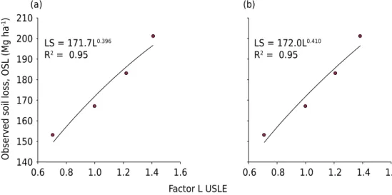
The values of SL observed showed a satisfactory relationship with the L factor for the two versions of the model, the USLE and RUSLE (Figures 4a and 4b). The adjustment coefficient between the variables was significant (p≤0.01) in the two versions.
Figure 4. The relation between values of total soil loss (SL) observed in each treatment and the values of the L factor (a) of the USLE and (b) of the RUSLE (average of replicates).
Factor L USLE 140
150 160 170 180 190 200 210
Observed soil loss, OSL (Mg ha
-1)
LS = 171.7L0.396 R2 = 0.95
LS = 172.0L0.410 R2 = 0.95
(a) (b)
For the USLE, in situations in which the degree of slope of the terrain is equal to or greater than 0.05 m m-1, the relation between SL and the L factor should be: SL = a L0.5 (Wischmeier and Smith, 1978). In this equation, L represents the relation between two lengths of slope; a is the intercept of the relation and represents the SL observed in slope length (22.1 m); and b is the exponent that represents the effect of the degree of slope of the terrain. Thus, for the data observed, the value of 0.396 for the exponent b found in the relation (Figure 4a) satisfactorily approached the value proposed by Wischmeier and Smith (1978) for the USLE, which is 0.5.
For the RUSLE, under the conditions of the study, the value of the exponent b in the equation of the factor L, calculated according to equations 2, 3, and 4, would be 0.487. The equation adjusted for the SL observed versus the L factor resulted in a value of 0.410 (Figure 4b). Thus, the value of b, of 0.410, found in the RUSLE version was closer to the calculated value (0.487) for this version than that observed for the USLE version (Figure 4a). The relatively small difference between the estimated and observed values for the USLE and RUSLE (Figures 5a and 5b, respectively) means that for the conditions of the study, the two versions estimated the SL with good approximation to the observed losses, constituting appropriate tools for prediction of SL, especially the RUSLE. Both versions of the model, but mainly the USLE, underestimated the SL. As for the effectiveness of the model, there was little variation between the observed data and the estimated data, especially in the largest slope lengths, as also observed in the study by Tiwari et al. (2000). Comparing the SL estimated by the USLE and RUSLE in plots under natural rain conditions, the authors found that, in general, the efficiency of the model was low for low values of SL, while for high SL, the efficiency was high. The results obtained for the RUSLE agrees with that obtained by Cecílio et al. (2009) in a study in a hydrographic micro basin of Viçosa, Minas Gerais, Brazil, in a Latossolo Vermelho-Amarelo (Oxisol); it was observed that the model underestimated the SL. The results also agree with Spaeth et al. (2003), who, in results obtained by using simulated rainfall, showed a strong tendency of the RUSLE to underestimate the SL. Risse et al. (1993) and Nearing (1998) verified that two versions of the model tended to overestimate the SL when they occurred in small quantities and to underestimate when in large quantities. The tendency of the USLE and RUSLE to underestimate SL disagrees with the results obtained by Amorim et al. (2010), who found a tendency of overestimation of SL by the models, regardless of the amount of soil lost.
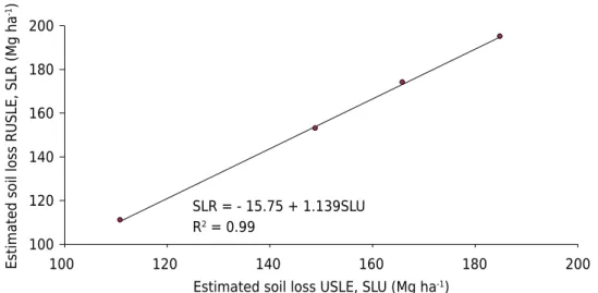
There were no significant differences in the estimated values of SL using the USLE and RUSLE for the different slope lengths in the study (Figure 6), meaning that both versions of the model turned out to be useful tools for SL prediction under the conditions evaluated.
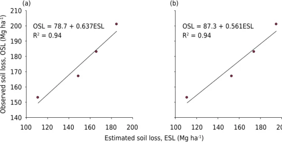
Figure 5. Relation between the values of observed soil loss (OSL) and the values of estimated soil loss (ESL); estimates made (a) by the USLE and (b) by the RUSLE in each treatment (average of replicates).
100 120 140 160 180 200
140 150 160 170 180 190 200 210
Estimated soil loss, ESL (Mg ha-1) OSL = 78.7 + 0.637ESL
R2 = 0.94 R2 = 0.94
(a)
100 120 140 160 180 200
OSL = 87.3 + 0.561ESL (b)
Observed soil loss, OSL (Mg ha
The use of this model in the USLE and RUSLE versions for SL prediction was only possible because of a database covering more than 20 years for the area under study. It should be noted that this erosion model was developed in temperate environments, to which its parameters were fitted, conditions quite different from the climate and soil conditions found in subtropical and tropical climates. Thus, according to Amorim (2003), it is essential to carry out a performance evaluation of this model when applied to Brazilian conditions before it is extensively used for prediction of SL. In addition, it is recommended that more water erosion studies be carried out under both natural rainfall and simulated rainfall conditions in different regions of the country so as to form a national database that allows use of this model throughout Brazil. It should be noted that problems related to underestimations or overestimations of SL values can be partially mitigated when more research is done so that all the values of the factors influencing erosion become known for different locations.
CONCLUSIONS
In the range between 11 m and 44 m, the soil losses by erosion are related in a positive and linear manner with an increase in slope length.
Water losses are related to rain amount; and soil losses are related to water loss and to the EI30.
Soil losses estimated by the USLE and RUSLE model have lower values than those observed experimentally in the field for bare soil at slope lengths between 11 m and 44 m, particularly the values estimated by the USLE.
The values of the L factor calculated for slope lengths of 11 m, 22 m, 33 m, and 44 m for the two versions (the USLE and RUSLE) of the soil loss prediction model show satisfactory results in relation to the soil loss values observed.
REFERENCES
Akeson M, Singer MJ. A preliminary length factor for erosion on steep slopes in Guatemala and its use to evaluate “curvas a nivel”. Geoderma. 1984;33:265-82. https://doi.org/10.1016/0016-7061(84)90029-6
Amaral AJ, Cogo NP, Bertol I. Comprimento crítico de declive e erosão hídrica, em três doses de resíduo cultural e dois modos de semeadura direta. Rev Cienc Agrovet. 2014;13:130-41.
Figure 6. Relation between values of soil loss estimated by the RUSLE (SLR) and estimated by the USLE (SLU) in each treatment (average of replicates).
100 120 140 160 180 200
100 120 140 160 180 200
Estimated soil loss USLE, SLU (Mg ha-1)
Estimated soil loss RUSLE, SLR (Mg ha
-1)
Amorim RSS. Avaliação dos modelos de predição da erosão hídrica USLE, RUSLE e WEPP para condições edafoclimáticas brasileiras [tese]. Viçosa: Universidade Federal de Viçosa; 2003. Amorim RSS, Silva DD, Pruski FF, Matos AT. Avaliação do desempenho dos modelos de predição da erosão hídrica USLE, RUSLE e WEPP para diferentes condições edafoclimáticas do Brasil. Eng Agríc. 2010;30:1046-9. https://doi.org/10.1590/S0100-69162010000600006 Bagarello V, Ferro V. Analysis of soil loss data from plots of differing length for
the Sparacia experimental area, Sicily, Italy. Biosyst Eng. 2010;105:411-22. https://doi.org/10.1016/j.biosystemseng.2009.12.015
Barbosa FT, Bertol I, Werner RS, Ramos JC, Ramos RR. Comprimento crítico de declive relacionado à erosão hídrica, em três tipos e doses de resíduos em duas direções de semeadura direta. Rev Bras Cienc Solo. 2012;36:1279-90. https://doi.org/10.1590/S0100-06832012000400022
Bertoni J, Pastana FI, Lombardi Neto F, Benatti Júnior R. Conclusões gerais das pesquisas sobre conservação do solo no Instituto Agronômico. Campinas: Instituto Agronômico; 1972. (Circular técnica, 20).
Bertol I, Almeida JA. Tolerância de perda de solo por erosão para os principais solos do estado de Santa Catarina. Rev Bras Cienc Solo. 2000;24: 657-68. https://doi.org/10.1590/S0100-06832000000300018
Bertol I, Barbosa FT, Mafra AL, Flores MC. Soil water erosion under different cultivation systems and different fertilization rates and forms over 10 years. Rev Bras Cienc Solo. 2014;38:1918-28. https://doi.org/10.1590/S0100-06832014000600026
Beutler JF, Bertol I, Veiga M, Wildner LP. Perdas de solo e água num Latossolo Vermelho Aluminoférrico submetido a diferentes sistemas de preparo e cultivo sob chuva natural. Rev Bras Cienc Solo. 2003;27:509-17. https://doi.org/10.1590/S0100-06832003000300012 Cecílio RA, Rodriguez RG, Baena LGN, Oliveira FG, Pruski FF. Aplicação dos modelos RUSLE e WEPP para a estimativa da erosão hídrica em microbacia hidrográfica de Viçosa (MG). Rev Verde Agroecol Desenv Sust. 2009;4:39-45.
Cogo NP, Levien R, Schwarz RA. Perdas de solo e água por erosão hídrica influenciadas por métodos de preparo, classes de declive e níveis de fertilidade do solo. Rev Bras Cienc Solo. 2003;27:743-53. https://doi.org/10.1590/S0100-06832003000400019
Cogo NP. Uma contribuição à metodologia de estudo das perdas de erosão em condições de chuva natural. I. Sugestões gerais, medição dos volumes, amostragem e quantificação de solo e água da enxurrada (1ª aproximação). In: Anais do 2º Encontro nacional de pesquisa sobre conservação do solo; 1978; Passo Fundo. Passo Fundo: Embrapa-CNPT; 1978. p.75-98.
Duley FL. Surface factor affecting the rate of intake of water by soils. Soil Sci Soc Am J. 1939;4:60-4.
Ellison WD. Soil erosion studies. Agric Eng. 1947;28:145-7, 197-201, 245-8, 297-300, 349-51, 402-5, 442-4.
Eltz FLF. Perdas por erosão sob precipitação natural em diferentes manejos de solo e coberturas vegetais. I. Solo da unidade de mapeamento São Jerônimo - 1ª fase experimental [tese]. Porto Alegre: Universidade Federal do Rio Grande do Sul; 1977.
Foster GR, Meyer LD, Onstad CA. An erosion equation derived from basic erosion principles. Trans Am Soc Agric Eng. 1977;20:678-82. https://doi.org/10.13031/2013.35627) @1977
Istok JD, Boersma L. Effect of antecedent rainfall on runoff during low-intensity rainfall. J Hydrol. 1986;88:329-42. https://doi.org/10.1016/0022-1694(86)90098-3
International Union of Soil Sciences/Working Group Word Reference Base - IUSS/WRB. World reference base for soil resources 2006. Rome: Food and Agriculture Organization of the United Nations; 2006. (World Soil Resources Reports, 103).
Laflen JM, Saveson IL. Surface runoff from graded lands of low slopes. Trans Am Soc Agric Eng. 1970;13:340-1. https://doi.org/10.13031/2013.38603
Lal R. Effects of slope length on erosion of some Alfisols in Western Nigeria. Geoderma. 1984;33:181-9. https://doi.org/10.1016/0016-7061(84)90054-5
Lal R. Effects of slope length on runoff from Alfisols in Western Nigeria. Geoderma. 1983;31:185-93. https://doi.org/10.1016/0016-7061(83)90012-5
Lal R. Effects of slope length, slope gradient, tillage methods and cropping systems on runoff and soil erosion on a tropical Alfisol: preliminary results. International Assoc. Hydrol Sci Publ. 1988;174:79-88.
Le Bissonnais Y, Cerdan O, Lecomte V, Benkhadra H, Souchere V, Martin P. Variability of soil surface characteristics influencing runoff and interrill erosion. Catena. 2005;62:111-24. https://doi.org/10.1016/j.catena.2005.05.001
Nearing MA. Why soil erosion models over-predict small soil losses and under-predict large soil losses. Catena. 1998;32:15-22. https://doi.org/10.1016/S0341-8162(97)00052-0
Reichert JM, Norton LD. Surface seal micromorphology as affected by fluidized bed combustion bottom-ash. Soil Technol. 1995;7:303-17. https://doi.org/10.1016/0933-3630(94)00015-V
Reichert JM, Norton LD, Huang C. Sealing, amendment, and rain intensity effects on erosion of high-clay soils. Soil Sci Soc Am J. 1994;58:1199-205. https://doi.org/10.2136/sssaj1994.03615995005800040028x
Rejman J, Usowicz B, Debicki R. Source of errors in predicting soil erodibility with USLE. Polish J Soil Sci. 1999;32:13-22.
Renard KG, Foster GR, Weesies GA, McCool DK, Yoder DC. Predicting soil erosion by water: A guide to conservation planning with Revised Universal Soil Loss Equation (RUSLE). Washington, DC: US Gov. Print Office; 1997. (Agricultural Handbook, 703).
Risse LM, Nearing MA, Laflen JM, Nicks AD. Error assessment in the universal soil loss equation. Soil Sci Soc Am J. 1993;57:825-33. https://doi.org/10.2136/sssaj1993.03615995005700030032x Rosa JD, Cooper M, Darboux F, Medeiros JC, Medeiros JC. Processo de formação de crostas superficiais em razão de sistemas de preparo do solo e chuva simulada. Rev Bras Cienc Solo. 2013;37:400-10. https://doi.org/10.1590/S0100-06832013000200011
Santos HG, Jacomine PKT, Anjos LHC, Oliveira VA, Oliveira JB, Coelho MR,
Lumbreras JF, Cunha TJF. Sistema brasileiro de classificação de solos. 3a ed. Rio de Janeiro: Embrapa Solos; 2013.
Schick J. Fatores R e K da USLE e perdas de solo e água em sistemas de manejo sobre um Cambissolo Húmico em Lages, SC [tese]. Lages: Universidade do Estado de Santa Catarina; 2014.
Schick J, Bertol I, Batistela O, Balbinot Júnior AA. Erosão hídrica em Cambissolo Húmico Alumínico submetido a diferentes sistemas de preparo e cultivo do solo. I - Perdas de solo e água. Rev Bras Cienc Solo. 2000;24:427-36. https://doi.org/10.1590/S0100-06832000000200019
Schick J, Bertol I, Cogo NP, Paz González A. Erosividade das chuvas de Lages, Santa Catarina. Rev Bras Cienc Solo. 2014a;38:1890-905. https://doi.org/10.1590/S0100-06832014000600024
Schick J, Bertol I, Cogo NP, Paz González A. Erodibilidade de um Cambissolo Húmico sob chuva natural. Rev Bras Cienc Solo. 2014b;38:1906-17. https://doi.org/10.1590/S0100-06832014000600025
Schick J, Bertol I, Barbosa FT, Miquelluti DJ. Erosão hídrica em Cambissolo Húmico submetido a diferentes sistemas de manejo. Rev Bras Cienc Solo. 2016. (Submitted)
Silva AM, Silva MLN, Curi N, Avanzi JC, Ferreira MM. Erosividade da chuva e erodibilidade de Cambissolo e Latossolo na região de Lavras, sul de Minas Gerais. Rev Bras Cienc Solo. 2009;33:1811-20. https://doi.org/10.1590/S0100-06832009000600029
Silva RL, De Maria IC. Erosão em sistema plantio direto: influência do comprimento de rampa e da direção de semeadura. Rev Bras Eng Agríc Amb. 2011;15:554-61. https://doi.org/10.1590/S1415-43662011000600003
Spaeth KE, Pierson Jr FB, Weltz MA, Blanckburn WH. Evaluation of USLE and RUSLE estimated soil loss on rangeland. J Range Manage. 2003;56:234-46. https://doi.org/10.2307/4003812
Tackett JL, Pearson RW. Some characteristics of soil crusts formed by simulated rainfall. Soil Sci. 1965;99:407-13.
Tiwari AK, Risse LM, Nearing MA. Evaluation of WEPP and its comparison with USLE and RUSLE. Trans Am Soc Agric Eng. 2000;43:1129-35. https://doi.org/10.13031/2013.3005
Wischmeier WH, Smith DD. Predicting rainfall erosion losses: a guide to conservation planning. Washington, DC: USDA; 1978. (Agricultural Handbook, 537).
Wischmeier WH, Smith DD. Rainfall energy and its relationships to soil loss. Trans Am Geophys Union. 1958;39:285-91. https://doi.org/10.1029/TR039i002p00285
Wrege MS, Steinmetz S, Reisser Júnior C, Almeida IR, editores. Atlas climático da Região Sul do Brasil: Estados do Paraná, Santa Catarina e Rio Grande do Sul. Pelotas: Embrapa Clima Temperado; Colombo: Embrapa Florestas; 2011.