Bank Failure and the Financial Crisis:
an Econometric Analysis of U.S. Banks
by
André Eduardo Paulo de Oliveira
Master Thesis in Finance and Taxation
Thesis Advisor:
Francisco Vitorino da Silva Martins, Ph.D.
Thesis Co-advisor:Elísio Fernando Moreira Brandão, Ph.D.
Biographical Note
André Eduardo Paulo de Oliveira was born on June 23rd, 1992, in Aveiro, Portugal.
He concluded his undergraduate studies in Management in 2013, at the University of Aveiro, with the final grade of 15. During that period he was a member of a Junior Enterprise with more than 20 people, which he later represented. In 2013, he was a summer intern at a bank.
André also did a summer internship in a small firm of strategic consulting and, while he was doing his Master’s Degree in Finance and Taxation at the School of Economics and Management, University of Porto, he did a professional internship at the same firm. Always looking for personal development, he is now learning Spanish.
Acknowledgments
About two years ago, I was starting one of the most challenging experiences of the personal and academic points of view, a challenge that one day was written in a notebook’s list and which, following the rules, should be scratched out, meaning thereby, challenge accomplished.
Despite the route not being that easy, due to some issues which today I overcame, the development of this investigation was fully involved in self-determination, always looking forward to present a successful research.
However, presenting this project would not even be a possibility without the contribution of Professor Francisco Vitorino Martins, whose incessant availability, technical knowledge and affection for the subject were really precious.
I also would like to thank the remaining Professors from the Master’s Degree Scientific Board, which is led by Professor Elísio Brandão, for the important preparation also given to this stage.
Lastly, I would like to mention my friends, the ones who have supported me when it was needed, and my family, which was absolutely crucial on the achievement of this goal, helping me to keep the focus along the journey.
Abstract
The analysis of bank failures enables the construction of models responsible for an earlier detection from banks with a high probability of being unsound, allowing a preventive behavior. Therefore, this paper uses first a data set of Federal Deposit Insurance Corporation (FDIC) insured U.S. banks from 2000 to 2014, in order to understand the most relevant indicators when it comes to explain bank failures. Results were then compared with those from a special sub-sample, called “crisis sample”, which comprises the period of more failures, from 2008 to 2014. In addition to the indicators’ proposal, combining CAMEL and non-CAMEL ones, applying the Principal Components Analysis and the Logistic Regression also allowed to discover that CAMEL indicators have a quite consistent role when it comes to explain bank failures during periods of financial instability. The increasing of the impact of Management Quality factor during the financial crisis should also be noticed.
JEL Classification: G01, G21, G28, G33
Keywords: Bank Failure, Financial Crisis, CAMELS, Principal Components Analysis, Logistic Regression
Index
1. Introduction ...1
2. Literature Review ...4
3. Methodology ... 10
3.1 Data and Sample ... 10
3.2 Variables ... 11
3.3 Model Specifications ... 13
4. Empirical Results ... 15
4.1. Principal Components Analysis ... 15
4.2. Logit Regressions and analysis to the whole sample ... 16
4.3. Logit Regressions and analysis to the “crisis sample” ... 20
5. Conclusions ... 23
Index of Tables
Table I: Number of Failed Banks per Year ... 10 Table II: Variable Definitions ... 12 Table III: Logit Regressions applied to the whole sample ... 17 Table IV: Summary of the Expected Influence from the Explanatory Variables .. 19 Table V: Logit Regressions applied to the “crisis sample” ... 21
1
1. Introduction
The role of banking system is quite determinant, especially when it comes to a nation’s economic growth and development. This phenomenon is more visible during a crisis, as it was example the subprime, when a considerable number of banks failed.
The beginning of the subprime crisis was firstly related to the inflation in the housing market, since people had to apply higher mortgages. Then, it was offered a subprime rate to people who didn’t fulfill the requirements (a riskier process) of the prime one, enabling them to afford the house anyway. Consequently, and because of the easiness of meeting the conditions to get the lending, an increase in homeownership was generated. However, the strong decrease of house prices as of 2006 led banks to bankruptcy.
Crisis, such as the one mentioned above, motivate, on the one hand, supervisors and regulators and, on the other hand, researchers to study even more how to predict and avoid failures or, at the same time, how to minimize its impacts.
The assessment of bank’s financial health can be done over two different perspectives: on-site and off-site examinations.
The first one, which involves all kinds of banks operations, is quite expensive, which means it is hardly applied with a suitable frequency. However, it doesn’t mean that on-site examinations are not applied to evaluate the soundness of banking institutions. They are and, as a result, they culminate with the attribution of a CAMELS rating. The rating varies between 1 and 5, where 1 and 2 illustrate low failure likelihood and 3, 4 and 5 the opposite. A bank’s poor rating will result in regulatory measures and, if it is not enough, a failing bank letter will be sent to the Federal Deposit Insurance Corporation (FDIC) by the regulator, starting a resolution.
After requesting loan and deposit data and visiting the bank in order to collect information, in person, FDIC has to decide which resolution structure it should opt for. Although the most applied one is purchase and assumption, in which bank’s assets and liabilities are auctioned, there is also deposit pay off. FDIC only uses to select the second one when there are no bidders available.
In contrast, off-site monitoring is essentially supported by financial statement data and regulatory reports, which reduces the process cost. As a result, a more
2 comprehensive number of banks have the possibility to be supervised and with a higher frequency.
Therefore, the purpose of this research - based on an off-site perspective - is to understand which variables explain bank failures in the U.S., using recent data and specific bank variables from FDIC database. The option for the U.S. market is connected to three arguments: the preponderance of its economy, the quantity of banks and the availability of its default information when comparing to any other country.
Moreover, this research contributes to the existing literature through the parallelism or aggregation of four purposes. The first one is the fact that it has been triggered from the connection of a comprehensive literature on banking bankruptcy. The second is related to the combination of methodologies applied, Principal Components Analysis and Logit model. The third one is based on the type of data that is used, specific bank information collected from Federal Deposit Insurance Corporation (FDIC). The last one is the period of time covered by the study, a more comprehensive and, at the same time, recent one.
This research comprises a whole sample, from 2000 to 2014, and a special sub-sample, called “crisis sample”, from 2008 to 2014.
Finally, in this study were used CAMELS and non-CAMELS variables. The acronym stands for Capital Adequacy, Asset Quality, Management Quality, Earnings Ability, Liquidity and Sensitivity to Market Risk. The Non-CAMELS group comprised measures such as credit risk, profitability, tax, growth and size.
Results from the whole sample period highlighted that the ratios of Equity to Total Assets, Net operating Income to Assets, Interest Expense to Interest Income, Net Loans and Leases to Deposits, Noncurrent Assets plus Other Real Estate Owned to Assets, Interest Expenses to Total Liabilities, both belonging to the CAMEL group are quite relevant to explain bank failure. Furthermore, the non-CAMEL ratios of Net Interest Income to Total Assets (representing Profitability) and Loan Loss Allowance to Total Assets (representing Credit Risk) also have an important role to explain bank default. The non-CAMEL ratio of Bank Size is still considered.
Besides, results from the “crisis sample” demonstrate the prominence of CAMEL indicators when it comes to explaining bank failures associated to the last financial crisis in U.S., given the focus of the explanatory power in these variables. Moreover, the
3 demand of a good management during the period of financial instability is also something to take into consideration and which is properly explained during this investigation.
Lastly, a final remark is given related to the capability of the indicators selected by the methodology to represent a wider dimension of information.
The reminder of this research proceeds as follows. The next section presents the literature review. The third section deals with methodology, incorporating also data and some issues about the variables. Then, section four presents the empirical results. Finally, the last section summarizes and concludes the findings of this study.
4
2. Literature Review
The study of bank failure prediction requires a consistent basis of available information. Probably economic and financial crisis are the most powerful sources of applicable knowledge when it comes to understand how to minimize its own consequences.
However, these complex phenomenons also allow the development of literature on banking with the addition of new perspectives and conclusions. Fahlenbrach et al. (2012), for example, classified poor stock return performance of a bank, over the 1998 crisis, as a powerful predictor of poor performance and as a way of forecast a failure during recent financial crisis.
Beltratti and Stulz (2012) connected the impact of governance and regulation to the credit crisis and found that banks with better governance and more fragile financing had a worse performance during the crisis.
Falenbrach and Stulz (2011) also analyzed Chief Executive Officer (CEO) incentives in the perspective of the credit crisis. They found no evidence that a better alignment between the interests of CEOs and shareholders would lead to higher bank stock returns. In fact, they found the opposite.
Lastly, Aebi et al. (2012), addressing an issue related to the corporate governance structure, found that when the Chief Risk Officer reports directly to the board of directors, banks have a better performance during credit crisis.
As it was highlighted there are several studies and preponderant conclusions arising from bank failure literature and it was only made reference to a few authors related to this perspective.
In fact, the literature on bank failure prediction and its accuracy has recently become much broader, including a diversity of failure prediction models. Some of them are going to be explored below.
In spite of the increasing concern about bank distress, firms’ failure forecast dates back to 1960s, when Beaver (1966), one of the first researchers to study bankruptcy prediction, presented a univariate approach of discriminant analysis in order to investigate the predictive ability of financial ratios.
5 Nonetheless, his work was extended by Altman (1968), who, using a multivariate discriminant analysis, assessed the relationship between failure and five financial indicators: working capital to total assets, retained earnings to total assets, earnings before interest and taxes to total assets, market value of equity to total debt and sales to total assets.
Although the use of discriminant analysis has dominated researches until the end of 1970s, a new approach was coming. The most intrinsic reason was the fact that model bases, such as financial data normally distributed and equality of variance-matrix of failed and non-failed banks, were often being violated (Taran, 2012).
Thus, Martin (1977), examining commercial banks introduced the logit model. This methodology, which has associated more than one period of observations, was proved to have a better predictive power than, for example, Discriminant Analysis and other one-period models.
However, focusing on Martin’s (1977) work, he started with twenty-five variables which were allocated to four groups: asset quality, liquidity, capital adequacy and earnings. His final model only had four ratios, which were represented by asset quality, capital adequacy and earnings groups.
Avery and Hanweck (1984), in their research, reinforce the group classification made by Martin (1977). Barth et al. (1985) suggest an extension to the model, with the use of liquidity. In their study, liquidity was estimated by the ratio of liquid assets to total assets and by the natural logarithm of the total assets.
Graham and Horner (1988) refer the influence of an adequate management and, following them, Thomson (1991), with a logit model prediction, evaluated and proved that bank failure is a consequence of the five factors, adding management quality as the fifth factor.
Despite the successive and progressive conclusions from authors, related to the influence and significance of variables linked to the factors quoted above, U.S. regulators had already introduced the CAMEL rating system in order to assess individual banks’ health.
At this moment, it is more intuitive that the acronym CAMEL stands for Capital adequacy (which shows the extent to which banks are able to absorb losses), Asset Quality (which includes risk diversification; a note for the fact that holding inferior
6 quality assets means being more vulnerable to losses), Management Quality (which takes into account the productivity and the management competence as the inverse of failure likelihood; a note for the fact that Management Quality being a hard factor to quantify), Earnings Ability (which have an ambiguous interpretation: a high operational performance vs. a high portfolio risk, however the sustainability of profits is also taken into account) and Liquidity (a low level is risky against a considerable deposit withdrawal but, on the other hand, a high level means poor management), however it somehow has evolved into CAMELS, which includes the addition of Sensitivity to Market Risk (which shows the impact on banks from, for example, fluctuations in the financial market), addressed by a few researchers.
Returning to methodologies, logit models are proved to have a good performance when it concerns to failure prediction and they are still very used in the modern literature, being Estrella et al. (2000), Arena (2008) and Andersen (2008) examples of that. The last one was focused, once again, on the determination of the best predictors of banks failure but, this time, on a Norwegian perspective.
In fact, following the vast literature, logit as well as probit models are able to predict banks’ failure probability, having diverse authors that discuss and test which one best succeeds.
Despite forecasting the probability of bank failure, they don’t determine exactly the moment of failure. Nevertheless, Cox (1972) proposed a solution, Cox proportional hazards model which following Ploeg (2010) have a similar predictive power.
Hazard analysis was used by several authors, such as Shumway (2001), who demonstrated that this methodology outperforms the traditional models, or Wheelock and Wilson (2000). Arena (2008), mentioned above, used both logit and hazard models to investigate bank failures in East Asia and Latin America.
In addition, many more predictive models co-exist. Kolari et al. (2002), for example, use logit and trait recognition, a nonparametric approach described as useful on small samples, to predict large U.S. commercial bank failures, based on data from one year and two years prior to the failure. They find that trait recognition could be a notorious early warning system for large failing banks. On the other hand, Lanine and Venet (2006) extend both methodologies to the Russian context and conclude that
7 although logit and trait recognition perform well, in this context the second outperforms the logit model.
Another model is the called neural networks, firstly used for bankruptcy classification by Odom and Sharda (1990), who used the variables found as significant by Altman (1968) and infer that it, at least, was as precise as discriminant analysis. However, Tam and Kiang (1992) were the first to apply this methodology to banks’ failure prediction. Furthermore, Celik and Karatepe (2007) also applied this model, but to the Turkish case.
Recently, Mayes and Stremmel (2013), with data from 1992 to 2012 from the FDIC for the US, analyzed the performance of different indicators of capital adequacy. Using at first a logit approach and then a Cox proportional hazard estimation, they found that the leverage ratio outperform risk-weighted capital. Furthermore, the leverage ratio, which is a better indicator because it is harder to manipulate, has best results when it comes to complex banks.
Sy et al. (2011), using a Cox proportional hazards model (and a probit model as a benchmark), added non-CAMEL variables extracted from Bankscope database, such as bank’s business structure indicators, off-balance sheet items, derivative investments and credit risk, to assess bank performance. Focusing on nine Central and East Asian countries, they identified a predictive power associated to bank’s derivative investments and credit risk. However, they also realized that business structure ratios and off-balance sheet items don’t fit the sample predictive function.
Jordan et. al. (2010) argue that bank’s failure risk can be detected up to four years prior to failure, since, with a multiple discriminant analysis, their study enabled them to predict US bank failures (for banks which failed between February 2, 2007 and April 23, 2010 and data from FDIC web site) with 66 % accuracy four years prior to failure, 71,4 % three years prior to failure, 78,6 % two years prior to failure and 88,2 % one year prior to failure. Moreover, they proved that the seven indicators referred below can be used to predict bank failure: ratio of non-interest income to interest income, ratio of non-accrual assets plus owned real estate “ORE” to total assets, ratio of interest income to earning assets, ratio of Tier One capital to total assets, Bank Holding Company dummy variable representing whether or not the bank is part of a holding company,
8 Savings Bank dummy variable representing whether or not the bank is a savings bank and MSA dummy variable representing whether or not the bank is located in a “Metropolitan Statistical Area”. Finally, they found that the ratio of real estate loans as a percentage of total assets is a strong predictor of bank failure.
Vilén (2010) conducted a study on U.S. Commercial Banks, from 2004 to 2009, with total assets worth more than 500 million dollars, whose variables were collected from FDIC database. The author started with thirty two variables and after performing the Student’s t-test and single variable logit analysis there were only twenty five independent variables. However, there was still the need to solve the multicollinearity problem whereas the final model included the following variables: nonaccrual rate, loan diversification, return on equity, capital growth, tax exposure, CMO ratio, uninsured deposits, risk free securities, dividend rate, loan growth, assets variation and liquid assets. Consequently, the author referred that previous researches’ findings are still applicable on bank’s failure prediction.
Poghosyan and Cihák (2009) carried out a research in European Union (EU-25) with financial data from Bureau Van Dijk’s BankScope database and NewsPlus database for the period of 1997-2007. They started with CAMEL factors and then they added others related to: depositor discipline, contagion effects, macroeconomic environment, banking market concentration and financial market. Using several versions of the logistic probability model, they found that the probability of default is negatively associated with the level of capitalization and earnings. Furthermore, they argue that the probability of default is inversely related to asset quality whereas management quality and liquidity seem not be significant. Finally, they concluded that contagion effects are important when predicting EU bank failures, in other words, it means that bank’s default probability is higher if there is a recent failure in a bank with similar size in the same country; and that stock prices may be relevant when one’s addressing bank’s default likelihood.
Montgomery et al. (2005) addressed Japan and Indonesia perspective with a logit analysis on financial ratios of commercial banks, whose data came from balance sheets and income statements. They used the following ratios: capital to deposits, equity to deposits, loans to equity, loans to capital, fixed assets to equity, fixed assets to capital, total equity capital to assets, return on equity, return on assets, liquid assets-shot term
9 borrowing to total deposits, equity to risk assets, loans to assets, treasury securities to assets, other securities to assets, capital to assets, core deposits to total liabilities, non-performing loans to total loans and total loan to total deposit. Consequently, they found the ratios loans to deposits and loans to total assets as the most significant when doing the forecasting of both countries’ bank bankruptcy. In the Indonesia case the ratio non-performing loans to total loans has predictive power, as well.
In summary, it’s explicit that there’s a diversity of methodologies coexisting, which are applied to different sets of countries. Databases vary according to the selected country and the period of time is also changeable.
Nevertheless, independent variables are, maybe, the most ambiguous determinant. Although CAMEL factors are globally accepted as decisive when predicting bank failure, ratios that represent each factor are still something that don’t gather total consensus. Furthermore, as it was verified, there are authors that inclusive add non-CAMEL variables, something that this research will follow.
10
3. Methodology
This section provides useful information related to the bank sample, the source of data, variables definitions, combination of methodologies applied and reasons why each one was selected.
Methodology chapter proceeds as follows: first, Data and Sample, then, Variables, and, finally, Model Specifications.
3.1 Data and Sample
This paper uses reports from the Federal Deposit Insurance Corporation (FDIC) statistics on depository institutions (SDI), available on its website. In addition, data were collected on an annual logic, from 2000 to 2014, covering only FDIC insured institutions.
Information for indicators calculation was obtained from the following global items: Assets and Liabilities, Income and Expense and Performance and Condition Ratios.
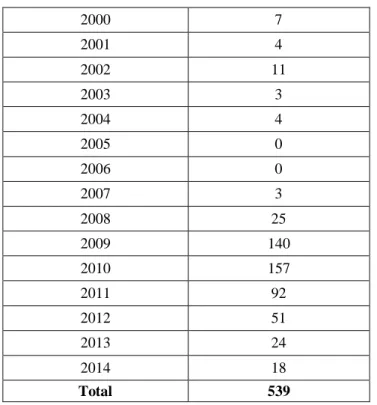
The number of failed banks per year, throughout the investigation period, is shown in Table I.
Table I: Number of Failed Banks per Year
2000 7 2001 4 2002 11 2003 3 2004 4 2005 0 2006 0 2007 3 2008 25 2009 140 2010 157 2011 92 2012 51 2013 24 2014 18 Total 539
11 Furthermore, the study comprises a dataset of 11.121 banks, which represents, during the whole sample period, a total of 128.261 observations, while “crisis sample”, a sub-sample from 2008 to 2014, represents a total of 54.411 observations. It’s also reasonable to point out that the number of banks is not constant over time, there are, as expected, market entries and exits.
3.2 Variables
In this investigation CAMELS and non-CAMELS variables will be used. Therefore, each one of the following factors is going to be represented by one or more indicators: Capital Adequacy, Asset Quality, Management Quality, Earnings Ability, Liquidity and Sensitivity to Market Risk. Besides, the non-CAMELS group comprises measures such as credit risk, profitability, tax, growth and size.
The dependent variable, based on the group of explanatory variables selected from the literature, represents the probability of bank failure.
There are two common strategies that can be applied when it involves variables. The first one consists on selecting a small set of variables which were indicated by earlier studies as being relevant. The second one, on the other hand, starts with a wide set of explanatory variables, including a more comprehensive list of risk factors (Ploeg, 2010).
This research follows the second strategy, applying a methodology in order to shorten the variables list - Principal Components Analysis - something that will be explained later.
Indicators presented in Table II were collected from the literature (Altman et al., 2014; Betz et al., 2014; Halling and Hayden, 2007; Mayes and Stremmel, 2013; Ploeg, 2010; Vilén, 2010; Wang and Ji, (unspecified)).
12 Table II: Variable Definitions
Source of the Definitions: Federal Deposit Insurance Corporation (FDIC)
Group
Designation Indicators
Formula with
FDIC Codes Definitions
(C)apital Adequacy
Equity/Total Assets EQV
Equity/Liabilities EQTOT / LIAB
Tier 1 Risk-based Capital Ratio1 RBC1RWAJ 1 Tier 1 capital as a percent of
risk-weighted assets.
Capital (Leverage) Ratio2 RBC1AAJ
2
Tier 1 capital as a percent of average total assets minus ineligible intangibles.
(A)sset Quality
Return on Assets ROA
Noncurrent Assets3 plus Other Real Estate Owned/Assets
NPERFV
3
Assets that are past due 90 days or more plus assets placed in nonaccrual status.
(M)anagement Quality
Net Interest Income/Number of Employees NIM / NUMEMP
Risk-weighted Assets Adjusted/Total Assets RWAJT / ASSET
Efficiency Ratio4 EEFFR
4
Noninterest expense less amortization of intangible assets as a percent of net interest income plus noninterest income.
(E)arnings Ability
Interest Expense/Interest Income EINTEXP/INTINC
Return on Equity ROE
Net Interest Margin5 NIMY
5
Total interest income less total interest expense as a percent of average earning assets.
Net Operating Income/Assets6 NOIJY 6 Net operating income as a
percent of average total assets.
(L)iquidity
Net Loans and Leases/Total Assets LNLSNTV
Interest Expenses/Total Liabilities EINTEXP / LIAB
Net Loans and Leases/Deposits LNLSDEPR
Domestic Deposits/Total Assets DEPDASTR
(S)ensitivity Volatile Liabilities/Assets VOLIAB / ASSET
Non-CAMELS
Loan Loss Allowance7/Total Assets LNATRES / ASSET
7
Reserve for loan and lease losses that is adequate to absorb estimate credit losses associated with loan and lease portfolio.
Net Interest Income/Total Assets NIM / ASSET
Cash Dividends/Total Assets EQCDIV / ASSET
Applicable Income Taxes/Total Assets ITAX / ASSET
Capital Growth [(EQTOT - EQTOT(-1)) /
EQTOT(-1)] x 100
Loan Growth [(LNLSNET - LNLSNET(-1)) /
LNLSNET(-1)] x 100
13 3.3 Model Specifications
Seeing that at the beginning a vast number of explanatory variables will be contemplated, one would say that it could lead to the multicollinearity problem, due to the probability of existing high correlations between variables.
In this research work, Principal Components Analysis will be applied with the ambition of minimizing redundant information. Therefore, it’s expected that it leads to the most comprehensive variables when it comes to explain banks’ failure. Furthermore, the principal components are not correlated, reducing the multicollinearity problem.
This method will be used first for CAMELS indicators and then it will be applied to non-CAMELS ones.
As it was mentioned before, after Martin (1977), logit model, became a widely applied methodology, especially when it concerns to literature about failure prediction and banking supervision (Andersen, 2008; Arena, 2008; Betz 2014; Li, 2013; Ploeg, 2010).
Consequently, and once it doesn´t assume multivariate normality among independent variables, which is a benefit since bank data uses to be not normally distributed (Vilén, 2010), the logit model will be applied in this research.
The utilization of logistic regression analysis implies that the failure probability relies on a vector of independent variables (Vilén, 2010; Ploeg, 2010). Moreover, the value of dependent variable varies between 1, for failed banks, and 0, for non-failed ones, since the model is characterized by being based on a cumulative function.
To sum up, in the proposed Logit models, the dependent variable is based on a group of explanatory variables selected from the literature and screened through a technical filter (Principal Components Analysis).
Associated to the logistic regression, standard errors are going to be estimated using Huber/White (QML) method. Thereby, standard errors are robust to certain misspecifications of the distribution from the dependent variable.
Following the results from Principal Components Analysis and applying the remaining methodology described above, equations will be first estimated with only
14 CAMELS and then also with non-CAMELS indicators. The more complex model, as it was said before, is the principal focus of this research, in order to gather the most efficient set of indicators to explain bank failures.
Finally, the last results will be compared with the period in which failures number was higher.
15
4. Empirical Results
Empirical Results comprise the analysis procedure and the results of the investigation, in other words, the explanation of the indicators’ screening process, the analysis of full sample results, looking for the most reliable indicators to explain bank failure, and the comparison with the sub-sample ones.
This chapter proceeds as follows: first, Principal Components Analysis, then, Logit Regressions and analysis to the whole sample, and, finally, Logit Regressions and analysis to the “crisis sample”.
4.1. Principal Components Analysis
The indicators’ screening process, Principal Components Analysis, is going to be explained below.
All the CAMELS indicators (eighteen), which were selected from the literature, were included in the first analysis. Only the first seven principal components have an eigenvalue higher than 1.00, which together explain over 65 % of the total variability in the data.
Thus, the indicators’ selection was made according to the following order: Equity to Total Assets (C), Net Operating Income to Assets (E), Interest Expense to Interest Income (E), Net Loans and Leases to Deposits (L), Net Interest Income to Number of Employees (M), Noncurrent Assets plus Other Real Estate Owned to Assets (A) and Interest Expenses to Total Liabilities (L).
The indicators’ selection was made, all along this procedure, by choosing the indicator with higher loading, on each principal component.
In conclusion, the first stage of the Principal Components Analysis culminated in seven indicators: one from Capital Adequacy, one from Asset Quality, one from Management Quality, two from Earnings Ability and two from Liquidity.
On the other hand, the non-CAMELS indicators (seven) were included in a second analysis, isolated from the CAMELS ones. After the application of the same procedure used in the first analysis, only the first three principal components have an eigenvalue higher than 1.00 and together these explain more than 56 % of the total variability in the data.
16 Up to now, the non-CAMELS indicators collected from this analysis have been the following: Net Interest Income to Total Assets, Bank Size and Capital Growth.
However, total variability explained by the two next components is so similar to the last one selected that it was decided to take the two associated indicators to the equation’s estimation phase, as well. Therefore, the five principal components explain over 83 % of the total variability in the data.
Finally, the two additional indicators were Loan Growth and Loan Loss Allowance to Total Assets.
4.2. Logit Regressions and analysis to the whole sample
Table III shows results from three logit regressions, whose main objective is to understand which variables explain banks’ failure (data from 2000 to 2014). Equation 1 represents the estimation of a first model, which only includes CAMELS indicators. In Equation 2, three other indicators were added, a result from the methodology above explained. Moreover, Equation 3 results from the addition of two more “other indicators”, following the reasons given above, as well.
17 Table III: Logit Regressions applied to the whole sample
Top number is the coefficient, bottom number is the p-value, and *, **, *** indicate statistical significance at the 10%, 5% and 1% level, respectively.
Indicators Equation 1 Equation 2 Equation 2.1 Equation 3 Equation 3.1
CAMELS Indicators Constant -1,050277 (0,0000)*** -2,407274 (0,0009)*** -1,665367 (0,0317)** -2,594043 (0,0042)*** -1,658302 (0,0329)** Equity to Total Assets -0,727173
(0,0000)*** -0,748189 (0,0000)*** -0,723298 (0,0000)*** -0,715763 (0,0000)*** -0,687288 (0,0000)*** Net Operating Income to
Assets -0,239284 (0,0000)*** -0,218578 (0,0000)*** -0,231961 (0,0000)*** -0,200369 (0,0000)*** -0,205044 (0,0000)*** Interest Expense to Interest
Income 0,998911 (0,0000)*** 0,876480 (0,0000)*** 0,909980 (0,0000)*** 1,051057 (0,0011)*** 0,854507 (0,0000)*** Net Loans and Leases to
Deposits -5,31E-0,6 (0,0560)* 5,01E-0,6 (0,0000)*** -1,26E-0,5 (0,0000)*** 3,57E-0,6 (0,0081)*** -1,25E-0,5 (0,0001)*** Net Interest Income to
Number of Employees -1,78E-0,6 (0,2855) -0,000668 (0,0000)*** - -0,000538 (0,0170)** -
Noncurrent Assets plus Other Real Estate Owned to Assets
0,150049 (0,0000)*** 0,146751 (0,0000)*** 0,146951 (0,0000)*** 0,127304 (0,0000)*** 0,124194 (0,0000)*** Interest Expenses to Total
Liabilities 0,030378 (0,0948)* 36,82906 (0,0000)*** 8,080554 (0,0000)*** 35,33310 (0,0000)*** 10,63981 (0,0000)*** Other Indicators
Net Interest Income to Total Assets -26,90044 (0,0000)*** -32,78557 (0,0001)*** -31,31569 (0,0068)*** -43,86838 (0,0000)*** Bank Size 0,138815 (0,0070)*** 0,121001 (0,0182)** 0,121244 (0,0307)** 0,097362 (0,0690)* Capital Growth -0,001003 (0,2711) - -0,000874 (0,2675) - Loan Growth -0,000524 (0,4773) -
Loan Loss Allowance to Total Assets 25,81164 (0,0001)*** 32,03025 (0,0000)*** McFadden R-squared 0,642378 0,660913 0,648699 0,664497 0,653780
Akaike info criterion 0,021914 0,022458 0,021548 0,022383 0,021257
Schwarz criterion 0,022614 0,023507 0,022334 0,023630 0,022131
Log likelihood -1194,134 -1107,886 -1175,243 -1095,051 -1158,244
LR statistic 4289,923 4318,745 4340,317 4337,720 4374,315
Prob(LR statistic) 0,000000 0,000000 0,000000 0,000000 0,000000
Obs with Dep=0 109189 99121 109390 98487 109390
18 According to the results presented in TableIII related to Equation 2, one realizes that all indicators, but Capital Growth, are statistically significant (at the 1% level). Therefore, Capital Growth indicator was removed. However, this removal contributed to a new not statistically significant indicator, Net Interest Income to Number of Employees.
Results from a second estimation are now presented in Equation 2.1. It shows six CAMEL indicators, both statistically significant at the 1% level, and two others, one statistically significant at the 5% level in a unilateral test and one statistically significant at the 1% level.
Following the same logic than before from Equation 3 to Equation 3.1, once all indicators but Loan Growth and Capital Growth had revealed to be statistically significant (all but Net Interest Income to Number of Employees and Bank Size at the 1% level), at the beginning Loan Growth was removed and then Capital Growth. However, after a new estimation one could verify that with the removal, Net Interest Income to Number of Employees indicator wasn’t statistically significant anymore. Then, the process was repeated and this indicator was removed.
Consequently, final results, covering six CAMEL indicators, both statistically significant at the 1% level, and three other ones, two statistically significant at the 1% level and one statistically significant at the 10% level in a unilateral test, are presented in the column of Equation 3.1.
The next stage is based on the analysis of Equation 2.1 and Equation 3.1, once, as it was explained above, both represent the final regression models, for the whole sample period. Table IV will be closely observed during the interpretation.
In both equations, the coefficient value of Equity to Total Assets is negative, as it was expected from the literature review. This means that a higher ratio reflects greater ability from banks to protect themselves against financial losses (loan losses or decreases in value of assets), resulting on a lower probability of bank failure.
The ratio Net Operating Income to Assets exhibits a negative coefficient, which follows the literature and means that a higher level of earnings decreases the probability of default.
19 Table IV: Summary of the Expected Influence from the Explanatory Variables
Interest Expense to Interest Income has a positive coefficient as it was predicted. It suggests that unsound banks have less ability to generate profits on interests, which increases the probability of default.
The coefficient of Net Loans and Leases to Deposits ratio presents a negative value. This finding is inconsistent with the literature, which argues that a higher value of the indicator may be connected with a lack of liquidity in order to face unforeseen obligations, increasing the probability of default. However, if the value of the ratio is too low, it could also mean that banks may not be earning as much as it is recommended. Thereby, a higher value of this indicator would result in a lower probability of default.
The positive coefficient of the Noncurrent Assets plus Other Real Estate Owned to Assets ratio is consistent with the investigation preliminary assumptions. It means that unsound banks usually have more non-performing loans, so that they are more likely to fail.
Indicators Influence Source
CAMELS Indicators
Equity to Total Assets - Betz et al. (2014); Wang and Ji (unspecified) Net Operating Income to
Assets - Mayes and Stremmel (2013)
Interest Expense to Interest
Income - Wang and Ji (unspecified); Ploeg (2010)
Net Loans and Leases to
Deposits + Mayes and Stremmel (2013)
Net Interest Income to Number
of Employees - Halling and Hayden (2007)
Noncurrent Assets plus Other
Real Estate Owned to Assets + Mayes and Stremmel (2013) Interest Expenses to Total
Liabilities + Betz et al. (2014)
Other Indicators
Net Interest Income to Total
Assets - Wang and Ji (unspecified)
Bank Size ? Wang and Ji (unspecified); Ploeg (2010); Li (2013)
Capital Growth - Vilén (2010)
Loan Growth - Vilén (2010)
Loan Loss Allowance to Total
20 Interest Expenses to Total Liabilities ratio also measures the cost of funds. Moreover, a higher value reveals problems in maintaining liquidity, which has led banks to take more significant risks. Consequently, banks with a higher value of this ratio are more likely to fail.
The coefficient value of Net Interest Income to Total Assets ratio is negative in both equations, following the literature. It also supports the thesis that sound banks have a greater ability to generate net interest income from its own assets, reducing their probability to get in trouble.
In spite of the inconclusive relation from literature between Bank Size and its failure probability, Equations 2.1 and 3.1 have a positive coefficient related to this indicator. At first sight, one would argue that large banks should have better diversified portfolios and then be less likely to fail. However, results show that maybe big banks are involved in risky lending activities, which had led them to huge losses.
Literature about the influence of Loan Loss Allowance to Total Assets ratio is also ambiguous, stating that, on the one hand, a higher value of this indicator means that banks are more prepared to loan default risks and, on the other hand, a higher value suggests that banks are expecting to experience significant cash flow losses related to their loan portfolios, results from Equation 3.1 are unequivocal. The positive sign from the coefficient supports the second perspective and shows that unsound banks have higher values of this ratio than the remaining ones.
4.3. Logit Regressions and analysis to the “crisis sample”
Equations 2.2 and 3.2, in Table V, result from Equations 2 and 3, respectively, but now the period of time analyzed varies between 2008 and 2014 since, as it is visible in table I, it was when the major number of failures occurred. Therefore, the main goal is to understand the most significant changes in terms of explanatory factors.
As a result, the two equations in the next table represent final solutions, after the removal of all statistically non-significant indicators.
21 Table V: Logit Regressions applied to the “crisis sample”
Top number is the coefficient, bottom number is the p-value, and *, **, *** indicate statistical significance at the 10%, 5% and 1% level, respectively.
Equation 2.2 presents six CAMEL indicators which are statistically significant at the 1% level and two non-CAMEL indicators, which are only statistically significant at the 10% level in a unilateral test.
Indicators Equation 2.2 Equation 3.2
CAMELS Indicators
Constant -0,013305
(0,9798)
-0,895633 (0,0001)*** Equity to Total Assets -0,769666
(0,0000)***
-0,782785 (0,0000)*** Net Operating Income to
Assets
-0,253396 (0,0000)***
-0,257710 (0,0000)*** Interest Expense to Interest
Income
0,940155 (0,0000)***
1,008179 (0,0000)*** Net Loans and Leases to
Deposits
-1,07E-0,6
(0,0000)***
-Net Interest Income to
Number of Employees -
-4,26E-0,6 (0,0805)* Noncurrent Assets plus Other
Real Estate Owned to Assets
0,097471 (0,0000)***
0,101659 (0,0000)*** Interest Expenses to Total
Liabilities 37,89336 (0,0000)*** 39,24315 (0,0000)*** Other Indicators
Net Interest Income to Total Assets -29,11883 (0,0674)* -Bank Size - - Capital Growth -0,000713 (0,0821)* - Loan Growth -
Loan Loss Allowance to
Total Assets -
McFadden R-squared 0,695189 0,693254
Akaike info criterion 0,037813 0,037920
Schwarz criterion 0,039626 0,039329
Log likelihood -804,6644 -809,9515
LR statistic 3670,431 3661,025
Prob(LR statistic) 0,000000 0,000000
Obs with Dep=0 42555 42607
22 Equation 3.2 presents six indicators, belonging all of them to the CAMEL group. Furthermore, all of them, but Net Interest Income to Number of Employees (statistically significant at the 10% level in a unilateral test), are statistically significant at the 1% level.
The coefficients sign from each indicator, in Equations 2.2 and 3.2, is the same which was verified before and was properly justified.
Nevertheless, in Equation 2.2, one of the statistically significant indicators at the 10% level (in a unilateral test) is a new one. Capital Growth indicator follows also what was expected from the literature, in other words, results allocate a negative sign to the coefficient, which means that banks with growing capital are usually in a better condition, keeping them off from a failure situation.
In Equation 3.2, the new indicator is Net Interest Income to Number of Employees, which is essentially an efficiency ratio. The higher the net interest result per employee is, the higher the efficiency of the bank and, as it is visible from the results, the lower the probability of failure. The arising of this indicator may be connected to the necessity of an efficient management during the period of financial crisis, as it was verified by Halling and Hayden (2007).
Finally, the prominence of CAMEL indicators must be highlighted when it comes to explaining bank failures associated to the last financial crisis in U.S., once it becomes more evident the concentration of the explanatory power in these variables, during the period of a higher number of bank defaults. In particular and dissecting Equation 3.2, it has one indicator from Capital Adequacy (Equity to Total Assets), one from Asset Quality (Noncurrent Assets plus Other Real Estate Owned to Assets), one from Management Quality (Net Interest Income to Number of Employees), two from Earnings Ability (Net Operating Income to Assets and Interest Expense to Interest Income) and one from Liquidity (Interest Expenses to Total Liabilities).
It also must be said that the resultant models incorporate very complete indicators. In addition to the five factors of CAMEL, which were stated in the last paragraph, Net Loans and Leases to Deposits was also used to represent the Credit Risk dimension in other studies. Moreover, Interest Expenses to Total Liabilities was used by Hasan et al. (2014) to represent Sensitivity to Market Risk, as well.
23
5. Conclusions
The recent financial turmoil has triggered so many significant losses for financial institutions and countless bank failures that it could only result in reexaminations of important issues, such as performance and soundness of banks, from academic and policy-makers.
This research focuses on obtaining the most efficient set of indicators to explain bank failures in the U.S. and in order to accomplish that it comprises a whole sample, from 2000 to 2014, and a special sub-sample, called “crisis sample”, from 2008 to 2014. Through a different combination of methodologies, thereby using the Principal Component Analysis and the Logistic Regression, and joining CAMELS with non-CAMELS indicators such as credit risk, profitability, tax, growth and size measures, this study goes further than the existent literature.
One of the main reasons behind the analysis of bank failures is the construction of models which are able to earlier detect signs of banks with a high probability of being unsound, allowing regulators to act in a preventive way against the damages in the economy.
Regression results from the whole sample period highlighted that the ratios of Equity to Total Assets, Net operating Income to Assets, Interest Expense to Interest Income, Net Loans and Leases to Deposits, Noncurrent Assets plus Other Real Estate Owned to Assets, Interest Expenses to Total Liabilities, both belonging to the CAMEL group,are quite relevant to explain bank failure. Furthermore, the non-CAMEL ratios of Net Interest Income to Total Assets (representing Profitability) and Loan Loss Allowance to Total Assets (representing Credit Risk) also have an important role on explaining bank default. The non-CAMEL ratio of Bank Size is still considered.
Moreover, the results from the “crisis sample” point out to the prominence of CAMEL indicators when it comes to explain bank failures associated to the last financial crisis in the U.S., given the concentration of explanatory power in these variables.
Besides, the arising of Net Interest Income to Number of Employees indicator (representing Management Quality) may be connected to the demand of a good management during the period of financial instability.
24 Finally, indicators resulting from final solutions are quite robust in terms of the diversity of information explained.
In this investigation, the effects of macroeconomic variables and financial market indicators weren’t taken into consideration due to the complexity of data collection. However, it’s something that, added to the present results and work concept, probably deserves further research.
One other way, may be connected to the adaptation of the work concept used, putting indicators which came from the results, the most relevant to explain bank failures, in a predictive basis model and so trying to understand its predictive power (from one to four years before, for example).
25
References
Aebi, V. et al. (2012), “Risk management, corporate governance, and bank performance in the financial crisis”, Journal of Banking & Finance, Vol. 36, pp. 3213-3226.
Altman, E. (1968), “Financial Ratios, Discriminant Analysis and the Prediction of corporate Bankruptcy”, Journal of Finance, Vol. 23, Nº 4, pp. 589-609.
Altman, E. et al. (2014) “Anatomy of Bank Distress: The Information Content of Accounting Fundamentals Within and Across Countries”, SSRN Working Paper.
Andersen, H. (2008), “Failure prediction of Norwegian banks: a logit approach”,
Norges Bank Working Paper.
Arena, M. (2008), “Bank Failures and Bank Fundamentals: A Comparative Analysis of Latin America and East Asia during the Nineties using Bank Level Data, Journal of
Banking and Finance, 32, pp. 299-310.
Avery, B. and A. Hanweck (1984), “A Dynamic Analysis of Bank Failures”, Bank
Structure and Competition Conference Proceedings, Federal Reserve Bank of Chicago,
pp. 380-395
Barth et al. (1985), “Thrift Institution Failures: Causes and Policy Issues”, Proceedings, Federal Reserve Bank of Chicago, pp. 184-216.
Beaver, H. (1966), “Financial Ratios and Predictors of Failure”, Journal of Accounting
Research, 4, pp. 71-102.
Betz, F. et al. (2014), “Predicting distress in European banks”, Journal of Banking &
26 Celik, E. and Y. Karatepe (2007), “Evaluating and forecasting banking crises through neural network models: An application for Turkish banking sector”, Expert Systems
with Applications, Vol. 33, pp. 809-815.
Cox, R. (1972), “Regression Models and Life-Tables”, Journal of the Royal Statistical
Society, 34, pp. 187-220.
Estrella, A. et al. (2000), “Capital Ratios as Predictors of Bank Failure”, Economic
Policy Review, Federal Reserve Bank of New York, 6, pp. 33-52.
Fahlenbrach, R. and R. Stulz (2011), “Bank CEO incentives and the credit crisis”,
Journal of Financial Economics, Vol. 99, pp.11-26.
Fahlenbrach, R. et al. (2012), “This time is the same: using banking performance in 1998 to explain bank performance during the recent financial crisis”, Journal of
Finance, Vol. 67, pp. 2139-2185.
Graham, C. and E. Horner (1988), “Bank Failure: An Evaluation of the Factors Contributing to the Failure of National Banks”, Proceedings, Federal Reserve Bank Chicago, pp. 405-435.
Halling, M. and E. Hayden (2007), “Bank Failure Prediction: A Three-State Approach”, Working paper, Oesterreichische National Bank and University of Utah.
Hasan, I. et al. (2014), “The Determinants of Global Bank Credit-Default-Swap Spreads”, Bank of Finland Research Discussion Papers.
Jordan, J. et al. (2010), “Predicting Bank Failures: Evidence from 2007 to 2010”, SSRN
Working Paper.
Kolari et al. (2002), “Predicting large US commercial bank failures”, Journal of
27 Lanine, G. and R. Venet (2006), “Failure Prediction in the Russian Bank Sector with Logit and Trait Recognition Models”, Expert Systems with Applications, pp. 463-478.
Li, Q. (2013), "What Causes Bank Failures During the Recent Economic Recession? ”,
Honors Project, Paper 28.
Martin, D. (1977), “Early Warning of Bank Failure. A Logistic Regression Approach”,
Journal of Banking and Finance, Vol. 1, pp. 249-276.
Mayes, D. and H. Stremmel (2013), “The Effectiveness of Capital Adequacy Measures in Predicting Bank Distress”, Presented at the Financial Markets and Corporate Governance Conference, 2013.
Montgomery et al. (2005), “Coordinated Failure? A Cross-Country Bank Failure Prediction Model”, Financial Stability Review, Vol. 5.
Ng, J. and S. Roychowdhury (2014), “Loan loss reserves, regulatory capital, and bank failures: Evidence from the 2008-2009 Economic Crisis”, Review of Accounting
Studies, 19 (3), pp. 1234-1279.
Odom, D. and R. Sharda (1990), “A Neural Network Model for Bankruptcy Prediction”,
International Joint Conference on Neural Networks, 2, 163-167
Ozel, G. and A. Tutkun (2013), “Probabilistic Prediction of Bank Failures with Financial Ratios: An Empirical Study on Turkish Banks”, Pakistan Journal of Statistics and Operation Research, Vol. 9, Nº 4, pp. 409-428.
Ploeg, S. (2010), “Bank Default Prediction Models: A Comparison and an Application to Credit Rating Transitions”, MA thesis, Erasmus School of Economics Rotterdam
Poghosyan, T. and M. Cihák (2009), “Distress in European Banks: An Analysis Based on a New Dataset”, IMF Working Papers.
28 Shumway, T. (2001), “Forecasting Bankruptcy More Accurately: A Simple Hazard Model”, Journal of Business, 74, pp. 101-124.
Sy, M. et al. (2011), “Bank Failure Prediction: Empirical Evidence from Asian Banks - Impact of Derivatives and Other Balance Sheet Items”, School of Economics, Finance and Marketing, RMIT University, Melbourne, Australia.
Tam, Y. and Y. Kiang (1992), “Applications of Neural Networks: The Case of Bank Failure Predictions”, Management Science, 38 (7), pp. 926-947.
Taran, Y. (2012), “What factors can predict that a bank will get in trouble during a crisis? Evidence from Ukraine”, MA thesis, Kyiv School of Economics.
Thomson, B. (1991), “Predicting Bank Failures in the 1980s”, Economic Review, Federal Reserve Bank of Cleveland, Vol. 27, Nº1, pp. 9-20.
Vilén, M. (2010), “Predicting Failures of Large U.S. Commercial Banks”, Master’s Thesis, Aalto University School of Economics.
Wang, X. and Z. Ji (unspecified), “Bank Failure Prediction: Empirical Evidence from US & UK Banks – Impact of Derivatives and Other Balance Sheet Items”, https://mediacast.blob.core.windows.net/production/Faculty/StoweConf/submissions/sw fa2014_submission_228.pdf, accessed on September 5, 2015.
Wheelock, C. and W. Wilson (2000), “Why do Banks Disappear? The Determinants of U.S. Bank Failures and Acquisitions”, The Review of Economics and Statistics, MIT Press, 82, pp. 127-138.