Studying elements ofgenetic programming for multiclass classification

(1)

UNIVERSIDADE DE LISBOA FACULDADE DE CI ˆENCIAS DEPARTAMENTO DE INFORM ´ATICA

STUDYING ELEMENTS OF GENETIC

PROGRAMMING FOR MULTICLASS

CLASSIFICATION

Jo ˜ao Eduardo Silva Pombinho Batista

MESTRADO EM ENGENHARIA INFORM ´

ATICA

Especializaç ão em Interaç ão e Conhecimento

Dissertac¸ ˜ao orientada por:

Prof. Dra. Sara Guilherme Oliveira da Silva

(2)

(3)

Are you doing anything next Saturday? We could go for a walk, or watch ducks and talk.

(4)

(5)

Agradecimentos

First of all, I would like to thank my advisor Sara Silva for all her support through these last two years. I would also like to thank her for allowing me to freely explore any approaches I came up with and using a part of her time to discuss them with me. I would also like to thank her for, when I was having doubts, reminding me which path I wanted to take my life to, and supporting my decisions.

A special thank to all the faculty members who, directly or indirectly, helped me through these five years with words of support, suggestions, by making an example of how good professionals work, or by explaining to me how the academic world works. Namely, my advisor Sara Silva, Francisco Martins, Jo˜ao Marques Silva, Paulo Urbano, and Ant´onio Branco.

I would also like to thanks everyone that both support and allowed me to delay the work done in my thesis. Namely, from the group ”Questões da Vida”, Filipe Pereira, João Cardoso, João Antunes, João Rodrigues, and Dharmite Prabhudas, from the group ”Fculianos”, João Becho, João Pinto, Tiago Correira, Francisco Araújo, Pedro Vieira, and Nuno Rodrigues, and everyone that I met during this last year, namely, Margarida Penedos, José Sousa, João Nobre, Kelly Silveira, Daniela Oliveira, and João Ye.

I would like to thank the Department of Informatics for allowing me to have the role of Monitor over this year and all my students, for their company over this year. Without them this year would have been way more monotonous.

A great thanks to those who took their time to read my thesis and give me suggestions on how I should improve my writing. Namely, my advisor Sara Silva, Filipe Pereira, Tiago Costa, M´ario Carvalho, and Nuno Rodrigues.

Last but not least, I would like to thank those who, although I haven’t been mee-ting very frequently, were inspiring, suppormee-ting, and always provided a great company. Namely, Lu´ıs Sampaio, David Silva, and my best friend, Ana Beatriz Alves.

(6)

(7)

Resumo

A classificação é tanto uma das mais fundamentais tarefas no que toca à tomada de decisões como um dos principais tipos de problemas que a aprendizagem automática tenta resolver. Ela encontra-se dividida em duas categorias, classificação binária e classificação multiclasse. O primeiro tipo pode ser facilmente resolvido de várias formas utilizando métodos já dispon´ıveis. Por outro lado, a classificação multiclasse requer métodos mais especializados, devido à alta complexidade dos problemas desta natureza. Outro pro-blema que este tipo de classificação enfrenta é que métodos como redes neuronais ou florestas aleatórias, apesar de serem os métodos que actualmente fornecem melhores re-sultados, podem não oferecer modelos facilmente interpretáveis.

Na implementação padrão de Programação Genética (PG), descrita em Genetic Pro-gramming: vol. 1, On the programming of computers by means of natural selection(1992) [3], cada indiv´ıduo é representado como uma árvore em que os nós não terminais contêm funções e os nós terminais contêm valores numéricos ou ´ındices para as caracter´ısticas de cada amostra, permitindo-lhes calcular valores em R quando lhes são dadas amostras de um conjunto de dados. Estes indiv´ıduos conseguem facilmente resolver problemas de regressão linear e de classificação binária. A classificação binária é tipicamente resolvida de uma forma simples. Por exemplo, num problema com uma classe A e uma classe B, o individuo pode associar a amostra à classe A se o valor obtido for negativo, caso contrario associará a amostra à classe B. Em (J. R. Koza, 2010) [7], é poss´ıvel ver que a PG tem ótimos resultados nestes dois tipos de problemas. No entanto, como foi dito anteriormente, um problema de classificação com múltiplas classes requer métodos mais especializados para obter bons resultados, fazendo com que a implementação padrão de PG não seja adequada para este tipo de problemas.

Apesar da PG nunca ter sido o método mais adequado para resolver problemas de classificação multiclasse, em (V. Ingalalli, 2014) [8], foi proposto um novo método, ba-seado em PG, que não só consegue ter bons resultados em classificação multiclasse, con-segue também devolver modelos interpretáveis. Este método, chamado M2GP (Multidi-mentional Multiclass Genetic Programming), é uma variante do algoritmo tradicional em que cada indiv´ıduo em vez de ter apenas um nó na sua raiz, tem vários nós. Esta alteração fez com que os indiv´ıduos em vez de devolverem um valor em R, devolvessem um valor em Rn. Agora os indiv´ıduos conseguem ter um espaço de sa´ıda com n dimensões onde

(8)

são representadas as amostras do conjunto de treino. A geometria deste espaço de sa´ıda permite que seja feita uma abordagem de classificação baseada em agregados, onde cada classe é representada pelo conjunto de coordenadas obtidas pelo indiv´ıduo quando lhe são dadas as amostras dessa classe. Neste tipo de classificação cada ponto é associado à classe cujo centroide se encontra mais próximo. O M2GP consegue ter resultados comparáveis aos dos perceptrões multicamadas e das florestas aleatórias. Desde a sua criação foram feitos melhoramentos ao algoritmo como o M3GP [4], o eM3GP [2] e o M4GP [20].

Neste projeto, iremos estudar o algoritmo M3GP. Este algoritmo é semelhante ao seu antecessor M2GP. A diferença entre as duas abordagens encontra-se no número de nós que um indiv´ıduo tem quando é criado e como é que esse número varia ao longo das gerações. No M2GP, os indiv´ıduos começam todos com um número preestabelecido de nós e esse número é mantido até ao final do treino. No M3GP, cada indiv´ıduo começa com apenas um nó na sua raiz, tal como no algoritmo padrão de PG, de forma a procurar soluções em espaços com menos dimensões nas primeiras gerações. À medida que as gerações passam, são usados operadores genéticos que permitem adicionar e remover dimensões aos indiv´ıduos, permitindo-lhes explorar espaços em dimensões superiores.

Apesar do M3GP dar resultados melhores que o seu antecessor, este continua a po-der ser melhorado. A implementação original deste algoritmo avalia os indiv´ıduos da população com base no número de amostras corretamente classificadas no conjunto de treino. Este método de avaliação tem dois problemas. O primeiro é que uma avaliação deste tipo não incentiva que haja uma evolução suave do espaço geométrico gerado por este indiv´ıduo. O segundo problema deve-se à complexidade da função utilizada para associar amostras a uma classe. Este algoritmo utiliza a distância de Mahalanobis [12] para associar as amostras à classe do centroide mais próximo. Usando esta distância, a complexidade do cálculo da distância de um ponto a um centroide em Rn é de O(n3), enquanto que a complexidade usando a distância Euclidiana é de O(n). O método usado para selecionar os operadores genéticos também pode ser melhorado. Na implementação original são usadas probabilidades fixas para escolher os operadores genéticos. Apesar desta abordagem dar bons resultados, da mesma forma que existem operadores que são inúteis na fase inicial da evolução, pode haver operadores que só são úteis em fases ini-ciais da evolução. Um exemplo seria o operador que remove nós da raiz dos indiv´ıduos no algoritmo M3GP, se os indiv´ıduos começam com apenas uma dimensão, este método é inútil na primeira geração. Selecionar estes métodos em etapas de evolução em que eles têm uma probabilidade reduzida de aumentar os resultados da avaliação dos indiv´ıduos pode, no m´ınimo, atrasar a evolução da população.

A primeira etapa deste projeto foi a implementação e validação do M3GP. Esta foi feita em Java [40] e tentou seguir à risca todas as especificações do algoritmo M3GP, descritas em M3GP - Multiclass Classification with GP (2015) [4], de modo a que esta pudesse ser validada replicando os resultados exibidos no artigo. Apesar dos indiv´ıduos

(9)

obtidos na nossa implementação serem maiores e com um maior número de dimensões, seguimos para a segunda e terceira etapas deste projeto quando os indiv´ıduos mostraram resultados que não eram necessáriamente piores em termos de número de amostras corre-tamente classificadas, tanto no conjunto de treino como no conjunto de teste. A diferença no tamanho dos indiv´ıduos pode ser devido ao M3GP original ter sido implementado usando o GPLAB [39], que utiliza medidas adicionais de controlo de inchaço [37, 38] por defeito.

A segunda etapa deste projeto foi a criação de novas funções de avaliação. Estas funções foram desenhadas com o objetivo de adotar uma função de avaliação que permi-tisse que a evolução do espaço de sa´ıda dos indiv´ıduos fosse mais suave. Para tal, em vez de usar uma função de avaliação baseada no número de amostras do conjunto de treino corretamente classificadas, passamos a usar uma função baseada em distância que tenta afastar os centroides dos agregados de amostras enquanto tenta puxar as amostras para o seu respetivo centroide. Havendo a necessidade de obter resultados em tempo útil, em vez de distância de Mahalanobis, foi usada a distância Euclidiana. Os resultados obti-dos foram comparaobti-dos com uma função semelhante à usada no algoritmo original, com a diferença de que esta usa uma função que associa as amostras ao centroide mais próximo usando a distância Euclidiana.

Das duas funções testadas nesta etapa, uma delas deu resultados péssimos e foi ime-diatamente ignorada. A outra função testada deu resultados equivalentes à função usada como ponto de comparação, não só no número de amostras corretamente classificadas, como no tamanho dos indiv´ıduos, no número de dimensões, e na evolução em geral, enquanto tem uma complexidade computacional inferior à função base. Durante esta fase tivemos um problema com a criação da função de avaliação dos indiv´ıduos. As distâncias tendem a ser maiores em espaços geométricos com um número de dimensões mais elevado, como tal foi necessário pensar numa forma de normalizar distâncias entre indiv´ıduos com diferentes numeros de dimensões. Esta tarefa foi feita com sucesso mas acreditamos que existirão funções que consigam fornecer melhores resultados.

A terceira etapa deste projeto foi alterar o método de seleção dos operadores genéticos de modo a que o programa inicialmente desse uma igual probabilidade a cada opera-dor genético de ser selecionado e, com o passar das gerações aprendesse que operaopera-dores genéticos melhoram, ou não, os indiv´ıduos. Desta forma, os operadores que estiverem a ser benéficos para os indiv´ıduos da população terão uma maior probabilidade de se-rem selecionados, enquanto que os operadores prejudiciais irão ter uma probabilidade reduzida. Numa segunda sub-etapa, foram também criados novos operadores genéticos, alegadamente maus, com o objetivo de estudar a evolução das suas probabilidades.

Os resultados obtidos além de indicarem melhorias significativas no número de amos-tras corretamente classificadas em metade dos conjuntos de dados utilizados, também indicaram que o cruzamento da versão padrão de PG é sempre útil e a sua utilidade tende

(10)

a aumentar com o passar das gerações. Também indicam que os operadores que trocam dimensões entre individuos tendem a perder a sua utilidade com o passar das gerações. Uma conclusão tirada nesta etapa final que serve de confirmação para observações fei-tas nas outras etapas é que as populações tendem a usar mais vezes o operador genético que muta o indiv´ıduo adicionando uma dimensão quando o conjunto de dados tem muitas classes. Por fim, foi proposto um novo método de cruzamento que troca as dimensões entre três indiv´ıduos. Este método, por ter uma maior probabilidade de seleção em todos os conjuntos de dados, mostrou ser prefer´ıvel ao cruzamento que troca as dimensões entre dois individuos.

Palavras-chave: Programação Genética, Aprendizagem Automática, Classificação, Multi-classe, Aglomeração Multi-dimensional

(11)

Abstract

Although Genetic Programming (GP) has been very successful in both symbolic re-gression and binary classification by solving many difficult problems from various do-mains, it requires improvements in multiclass classification, which due to the high com-plexity of this kind of problems, requires specialized classifiers.

In this project, we explored a multiclass classification GP-based algorithm, the M3GP [4]. The individuals in standard GP only have one node at their root. This means that their output space is in R. Unlike standard GP, M3GP allows each individual to have n nodes at its root. This variation changes the output space to Rn_{, allowing them to construct}

clusters of samples and use a cluster-based classification.

Although M3GP is capable of creating interpretable models while having competitive results with state-of-the-art classifiers, such as Random Forests and Neural Networks, it has downsides. The focus of this project is to improve the algorithm by exploring two components, the fitness function, and the genetic operators’ selection method.

The original fitness function was accuracy-based. Since using this kind of functions does not allow a smooth evolution of the output space, we tried to improve the algorithm by exploring two distance-based fitness functions as an attempt to separate the clusters while bringing the samples closer to their respective centroids.

Until now, the genetic operators in M3GP were selected with a fixed probability. Since some operators have a better effect on the fitness at different stages of the evolution, the fixed probabilities allow operators to be selected at the wrong stages of the evolution, slowing down the learning process. In this project, we try to evolve the probability the genetic operators have of being chosen over the generations. On a later stage, we proposed a new crossover genetic operator that uses three individuals for the M3GP algorithm. The results obtained show significantly better results in the training set in half the datasets, while improving the test accuracy in two datasets.

Keywords: Genetic Programming, Machine Learning, Classification, Multiclass, Multidimensional clustering

(12)

(13)

List of Figures

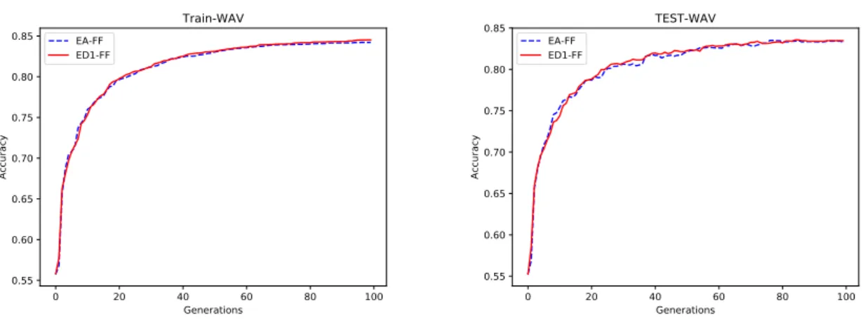
5.1 Evolution of training(left) and test(right) accuracies of the EA-FF and ED1-FF popula-tions when learning the WAV dataset. . . 37 5.2 Evolution of training(left) and test(right) accuracies of the EA-FF and ED1-FF

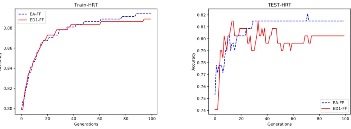
popula-tions when learning the YST dataset. . . 37 5.3 Evolution of training(left) and test(right) accuracies of the EA-FF and ED1-FF

popula-tions when learning the HRT dataset. . . 38 5.4 Evolution of training(left) and test(right) accuracies of the EA-FF and ED1-FF

popula-tions when learning the MCD3 dataset. . . 38 5.5 Evolution of probability of selection of the St-XO GO over the generations in all dataset,

using the EA-FF(left) and the ED1-FF(right), using the five original GOs. . . 45 5.6 Evolution of probability of selection of the Swap-dim GO over the generations in all

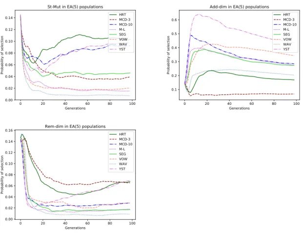
dataset, using the EA-FF(left) and the ED1-FF(right), using the five original GOs. . . . 45 5.7 Evolution of probability of selection of the St-Mut(left), the Add-dim(right), and the

Rem-dim(bottom) GOs over the generations in all dataset, using the EA-FF and the five

original GOs. . . 46

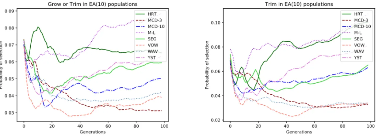
5.8 Evolution of probability of selection of the Swap-dim(left) and the Chop(right) GOs over the generations in all dataset, using the EA-FF and the ten GOs. . . 51 5.9 Evolution of probability of selection of the Grow or Trim(left) and the Trim(right) GOs

over the generations in all dataset, using the EA-FF and the ten GOs. . . 51 5.10 Evolution of probability of selection of the Swap-dim(solid line) and the Swap3-dim(dashed

line) GOs over the generations in the HRT and MCD-3 dataset, using the EA-FF and the

ten GOs. . . 51

A.1 Class Diagram section of the implementation used for the first stage of the project, referent to the initialization of the classifier . . . 67 A.2 Class Diagram section of the implementation used for the first stage of the project,

referent to the evaluation of the population’s individuals . . . 68 A.3 Class Diagram section of the implementation used for the first stage of the project,

referent to the usage of genetic operators. . . 68 xiii

(16)

B.1 Comparison of the number of dimensions between using the accuracy-based function (EA-FF) and using the distance-based function (ED1-FF), marked with *1, in the 8 datasets listed in 3.1. . . 69 B.2 Comparison of training accuracy between the original and our implementation

of M3GP, marked with *, in the 8 datasets listed in 3.1. . . 70 B.3 Comparison of test accuracy between the original and our implementation of

M3GP, marked with *, in the 8 datasets listed in 3.1. . . 71 B.4 Comparison of training accuracy on all datasets between using the Euclidean

Accuracy fitness function (EA) and using the first distance-based fitness function (ED1) . . . 72 B.5 Comparison of test accuracy on all datasets between using the Euclidean

Ac-curacy fitness function (EA) and using the first distance-based fitness function (ED1) . . . 73 B.6 Comparison of training accuracy on the HRT, and MCD3 datasets between using

the Euclidean Accuracy fitness function (EA), and using the first distance-based (ED1) fitness function, while using five genetic operators (5) and ten genetic operators (10). . . 74 B.7 Comparison of training accuracy on the MCD10, and M-L datasets between

us-ing the Euclidean Accuracy (EA) fitness function, and usus-ing the first distance-based (ED1) fitness function, while using five genetic operators (5) and ten ge-netic operators (10) . . . 74 B.8 Comparison of training accuracy on the SEG, and WAV datasets between using

the Euclidean Accuracy (EA) fitness function, and using the first distance-based (ED1) fitness function, while using five genetic operators (5) and ten genetic operators (10). . . 75 B.9 Comparison of training accuracy on the VOW, and YST datasets between using

the Euclidean Accuracy (EA) fitness function, and using the first distance-based (ED1) fitness function, while using five genetic operators (5) and ten genetic operators (10). . . 75 B.10 Comparison of test accuracy on the HRT, and MCD3 datasets between using

the Euclidean Accuracy (EA) fitness function, and using the first distance-based (ED1) fitness function, while using five genetic operators (5) and ten genetic operators (10). . . 76 B.11 Comparison of test accuracy on the MCD10, and M-L datasets between using

the Euclidean Accuracy (EA) fitness function, and using the first distance-based (ED1) fitness function, while using five genetic operators (5) and ten genetic operators (10). . . 76

(17)

B.12 Comparison of test accuracy on the SEG, and WAV datasets between using the Euclidean Accuracy (EA) fitness function, and using the first distance-based (ED1) fitness function, while using five genetic operators (5) and ten genetic operators (10). . . 77 B.13 Comparison of test accuracy on the VOW, and YST datasets between using the

Euclidean Accuracy (EA) fitness function, and using the first distance-based (ED1) fitness function, while using five genetic operators (5) and ten genetic operators (10). . . 77

(18)

(19)

List of Tables

3.1 Datasets used and their number of classes, attributes, and samples . . . 17

3.2 Parameters used on the runs by default . . . 18

3.3 Variables used in the fitness functions . . . 21 5.1 Comparison of results between the original implementation of M3GP and our

imple-mentation . . . 34

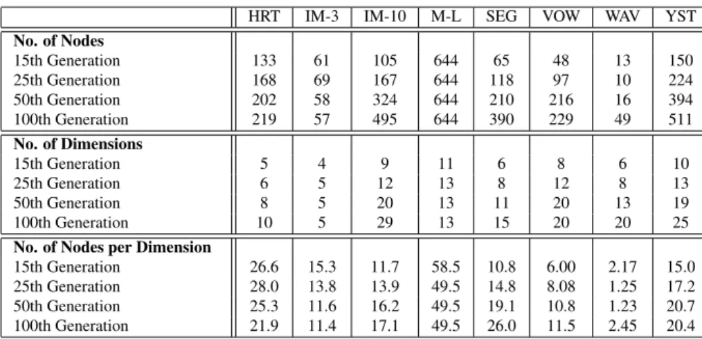
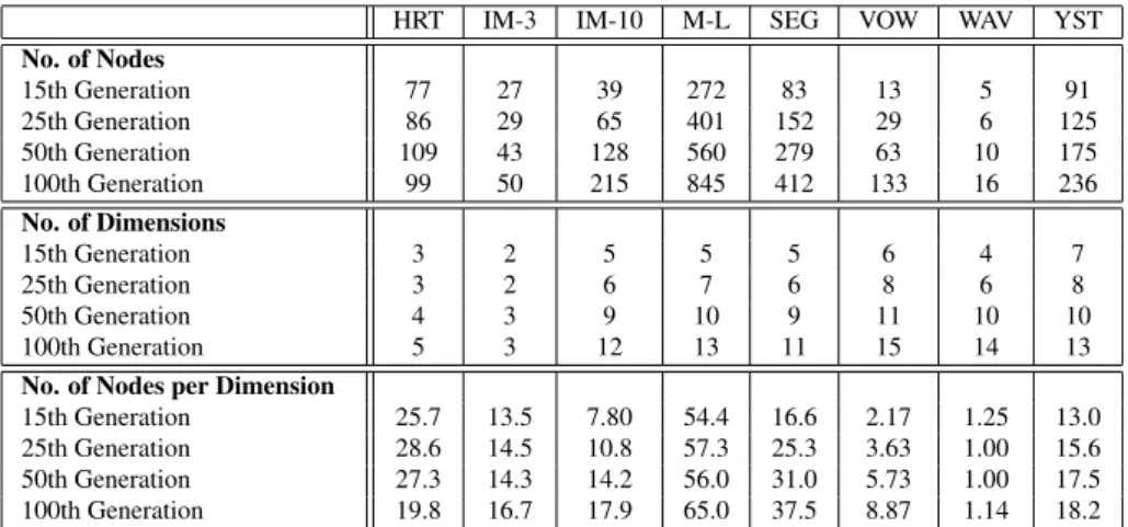
5.2 Evolution of the number of nodes and dimensions over the generations for our

imple-mentation . . . 35

5.3 Comparison of results between the different fitness functions . . . 36 5.4 p-values obtained by comparing the results from the populations learning the datasets

using the EA-FF and the ED1-FF. The underline is used to symbolize that the EA had a significantly better result than ED1.. . . 36 5.5 Evolution of the number of nodes and dimensions over the generations for the EA-FF . 39 5.6 Evolution of the number of nodes and dimensions over the generations for the ED1-FF . 39 5.7 Comparison between the average number of nodes, dimensions, and nodes per

dimen-sion of using the EA-FF and the ED1-FF, over all the datasets . . . 40 5.8 Comparison of results between the Euclidean Accuracy fitness function and the first

sigmoid fitness function for both five and ten genetic operators (GO) . . . 41 5.9 p-values obtained by comparing the results from the populations learning the datasets

using the EA-FF and the ED1-FF, with their respective counter part with 5 GOs with adaptable probabilities and these counterparts with the 10 GOs counterparts. The un-derline is used to symbolize that the first population has a significantly better result and bold symbolizes a worse result. . . 42 5.10 Evolution of the number of nodes, dimensions, and nodes per dimension over the

gener-ations for the EA-FF with five genetic operators . . . 42 5.11 Evolution of the number of nodes, dimensions, and nodes per dimension over the

gener-ations for the EA-FF with ten genetic operators . . . 43 5.12 Evolution of the probability of selection of the original genetic operators on all eight

datasets using the Euclidean Accuracy fitness function (EA-FF), and its standard deviation 47 5.13 Evolution of the probability of selection of the original genetic operators on all eight

datasets using the first distance-based fitness function (ED1-FF), and its standard deviation 48 xvii

(20)

5.14 Evolution of the probability of selection of the original five genetic operators when all ten genetic operators were tested, and their standard deviation. Results obtained from

using the EA-FF . . . 52

5.15 Evolution of the probability of selection of the new five genetic operators when all ten genetic operators were tested, and their standard deviation. Results obtained from using

the EA-FF . . . 53

5.16 Evolution of the probability of selection of the original five genetic operators when all ten genetic operators were tested, and their standard deviation. Results obtained from

using the ED1-FF . . . 54

5.17 Evolution of the probability of selection of the new five genetic operators when all ten genetic operators were tested, and their standard deviation. Results obtained from using

the ED1-FF . . . 55

(21)

Chapter 1 Introduction

The focus of this project is the study and improvement of the multiclass classification algorithm M3GP (Multidimentional Multiclass Genetic Programming with multidimen-sional populations), proposed in M3GP - Multiclass Classification with GP (2015) [4].

This chapter will first give a brief introduction about what Genetic Programming (GP) is, and then, we will explain why it’s worth to do research on Multiclass classification, why we are using genetic programming to do this kind of classification, how we will improve the M3GP algorithm, and what changes this project will bring to the GP field and the machine learning community.

1.1 Genetic Programming

As stated by Koza in Genetic Programming: On the programming of computers by means of natural selection(1992) [3], ”In nature, biological structures that are more suc-cessful in grappling with their environment survive and reproduce at a higher rate. Bi-ologists interpret the structures they observe in nature as the consequence of Darwinian natural selection operating in an environment over a period of time. In other words, in nature, structure is the consequence of fitness. Fitness causes, over a period of time, the creation of structure via natural selection and the creative effects of sexual recombination (genetic crossover) and mutation. That is, fitness begets structure.”. In nature, each indi-vidual has their own structure and behavior, even within the same population. Since each individual need to execute several tasks in order to survive and reproduce, individuals who are better prepared to execute these tasks will have a higher chance of survival and repro-duction while the other individuals, who are less fit for survival, will have a lower chance of survival and reproduction. This is the concept of survival of the fittest and natural se-lection described by Charles Darwin in On The Origin of Species by Means of Natural Selection(1859) [32]. Over many generations, the population as a whole comes to contain more individuals whose structure and behavior enable them to better execute their tasks and to survive and reproduce. Over time, the structure of the individuals changes because

(22)

Chapter 1. Introduction 2

of this natural selection that tries to raise their fitness.

Having this in mind, Genetic Programming (GP) is a machine learning approach where the main algorithm follows the principles of the Darwinian natural selection. This algorithm first receives a task and then creates a population of randomly generated pro-grams that will try to solve it. Although the most likely scenario is one where all these individuals will have a bad result in solving their task, some of these individuals will achieve better results and therefore a better fitness. The selection of individuals for re-production favors the individuals with higher fitness. This way, those individuals will be more likely to reproduce, leaving their offspring to the next generation. After a new generation of individuals is completed, these individuals are evaluated, and the process starts all over again, trying to improve the results of the population over the course of the generations.

1.2 Motivation

Classification is not only one of the most fundamental tasks in order to make decisions in real-world problems, it’s also one of the main type of problems in which machine learn-ing is used. This creates a great interest in improvlearn-ing the available methods to solve this kind of problems. Classification can be divided into two categories, binary classification, and multiclass classification. The first type can be solved in endless ways using many different available methods. Multiclass classification requires more specialized methods due to the high complexity of this kind of problems. Another problem it faces is that the best methods used, normally Neural Networks and Random Forests, don’t generate models that are ready to be easily interpreted by humans.

Although GP has not always been an adequate method for multiclass classification, in (V. Ingalalli, 2014) [8], a new GP-based method was implemented. This method not only gave good results in multiclass classification, it also provided interpretable models. This algorithm is a variation of the standard GP in which an individual is able to convert each sample into a point in Rn_{. The geometric properties of this kind of output space allow the}

individuals to use a cluster-based classification. This classification is made by creating a cluster for each class using the samples on the training set, converted to coordinates in the output space, an then associating the samples to the closest class centroid using the Mahalanobis distance[12]. This method, named M2GP (Multidimentional Multiclass Genetic Programming), had results comparable to those of the Multilayer Perceptron and the Random Forests. Since then, there have been a few variants the algorithm such as the M3GP [4], the eM3GP [2] and the M4GP [20].

The M3GP algorithm has two issues that motivate the study of an alternative fitness function. In its original state, M3GP uses a fitness function that not only doesn’t take into consideration the intra-cluster and inter-cluster distances but is also very expensive

(23)

in terms of computational complexity. This function uses the Mahalanobis distance which is very complex. To calculate the distance between two points in Rn_{, this function has a}

complexity of O(n3), while the Euclidean distance has a complexity of O(n).

Another issue with GP algorithms is that since the population selects the crossover and mutation genetic operators with a fixed probability, they might be selected on stages of the evolution where they are not needed. Using these genetic operators on the wrong stages can slow down the evolution. The variance of the importance of each genetic operator over the generations was already an issue in standard GP. Since the M3GP algorithm has more genetic operators, this problem is bound to be worse in this algorithm. This motivates us to try to solve this issue by adapting the probabilities that each genetic operator has of being selected to the needs of the population.

1.3 Goals

This project had three goals: 1) to implement the M3GP algorithm and replicate the results reported in (L. Mu˜noz, 2015) [4], 2) to make improvements in the fitness function of the M3GP algorithm, and 3) to automatically adapt the probabilities that each genetic operator has of being used during the evolution. These goals will be mentioned later as, respectively, the first, second, and third stages of this project.

The fitness function used by M3GP in (L. Mu˜noz, 2015) [4] was the classification accuracy. The accuracy of an individual was obtained by classifying each sample of the training set by associating it with the closest class centroid using the Mahalanobis dis-tance. In order to make an improvement to the fitness function, we are making an attempt to use a distance-based fitness function rather than an accuracy-based fitness function. To obtain results quickly the fitness functions we are testing use the Euclidean distance. The results are compared with the results obtained using an accuracy-based fitness function that uses the Euclidean distance.

To automatically adapt the probabilities that each genetic operator has of being used, we are changing the method of selection of the genetic operator to one that initially gives each genetic operator an equal chance of being selected. From this point, every time an individual uses an operator which improves the individual’s fitness, the probability of occurrence of that genetic operator will increase, otherwise, it will decrease. If the opera-tor doesn’t create changes on the individual’s fitness the probability will also decrease to avoid choosing useless operators. With this, the operators that are beneficial to the evo-lution will be used more often, while the prejudicial operators will be avoided, hopefully speeding learning.

(24)

1.4 Contributions

This project offers the following contributions:

• A full implementation of the M3GP (M2GP with Multidimensional Populations) method, written in Java [40] and ready to be used on Weka [6].

• New, and more efficient in terms of computational complexity, fitness functions were implemented and tested on the M3GP algorithm. A study over the results obtained by testing these fitness function was then made, in order to understand the differences in the accuracy, and on the evolution of the population when using different fitness functions.

• New methods for the automatic adaptation of the probabilities of selection of ge-netic operators were proposed and tested. A study was made on the influence of these adaptations on the accuracy of the population and on the evolution of the probabilities each genetic operator has over the generations.

In this project, we made a contribution to the GP community by validating the previ-ously obtained results using the M3GP, and by presenting alternatives that increase this algorithm’s efficiency by using different fitness functions and methods to select genetic operators. Since there are not many robust methods for multiclass classification that pro-duce an easily interpretable model, the improvement of the M3GP algorithm is an impor-tant contribution to the machine learning community in general.

1.5 Structure of the document

This document is organized with following structure:

• Chapter 2 - Describes some applications of the M3GP algorithm and other related implementations in real life problems. Some other methods with different ap-proaches are also mentioned such as non-clustering based GP methods and methods that rely on genetic programming to do feature evolution but use other clustering methods for classification.

• Chapter 3 - Contains information about the datasets and parameters used in each simulation and information about the algorithm used. The algorithm section is di-vided into three parts, the original algorithm, the modifications made to test new fitness functions, and the automatic adaptation of the genetic operator probabilities. • Chapter 4 - Describes the implementation made to run the classifier. It also includes

(25)

• Chapter 5 - Contains the results of all the runs made in this project and their analy-sis.

• Chapter 6 - Contains the conclusions of the project and discusses possible future work.

(26)

(27)

Chapter 2 Related work

In this section, we will mention some applications of GP algorithms such as classifica-tion, feature evoluclassifica-tion, and evolution of the probabilities of selection of genetic operators. The topics related with classification discussed in this section are the M3GP algorithms considered to be similar, other GP-based algorithms that use clustering techniques, non-clustering GP algorithms for multiclass classification, and real-world applications of GP algorithms to solve classification problems. There are many articles referring ways to use GP in multiclass classification, and many of these approaches use GP for feature evolu-tion, so the explanations about these topics will be brief. A longer explanation will be given on the papers related to the evolution of operator probabilities, as the topic will be studied further in this project and it seems to be a topic of importance with few recent works.

2.1 M3GP and other variants

Since there are many variants of the M3GP classifier, this section will cover some of those variants, namely its predecessor M2GP, its successor M4GP, its brother eM3GP, and another approach which can be considered as similar to the M3GP classifier for being cluster-based classifiers and using a similar method of classification.

A new GP framework, named Multi-dimensional Multiclass Genetic Programming (M2GP), was proposed in (V. Ingalalli, 2014) [8]. At the time, this method was a novel algorithm for tree-based GP where each individual could have n nodes at its root instead of only one, allowing the individuals to have an output space in Rn_{. The geometry of}

the output space allowed this GP method to use a cluster-based classification method and solve multiclass classification problems. This approach was tested on a large set of benchmarks problems from several different sources and was able to compete against the Multilayer Perceptron and the Random Forests, showing GP was able to solve this kind of problems.

The M3GP algorithm is very similar to the M2GP algorithm, the main difference 7

(28)

Chapter 2. Related work 8

being in the evolution of the number of dimensions in each individual. While the M2GP uses a fixed number of dimensions, established in the initialization of the classifier, the M3GP creates all individuals with only one dimension and the mutation operators allow each individual to create or destroy dimensions.

M4GP was presented in (La Cava W., 2017) [20] as a new classification method to evolve feature transformations. This is a stack-based GP system that allows each individ-ual to produce multiple outputs. Like M2GP and M3GP, this method has the advantage over typical classification methods of producing models that are easily interpretable by humans. The results obtained indicate that M4GP outperforms other GP methods for classification and performs competitively with other machine learning methods in terms of accuracy.

Like many other classifiers, M3GP appears to be suffering from overfitting, and is negatively affected by class imbalance, and also suffers from bloat on a dimensional level. A new method named ensemble M3GP (eM3GP) was proposed in (S. Silva, 2016) [2], intended to address some of the M3GP issues. Some variants of the eM3GP were tested and the results observed had competitive results with classifiers like Random Forests, Random Subspaces, and Multilayer Perceptron.

In (Smart W., 2004) [16], the authors describe a probability-based GP approach to multiclass classification problems. Although it’s not explicit that clustering methods are being used, the approach has several similarities with M2GP. This approach, instead of directly associating a sample to the class of the closest class centroid on the output space, uses a Gaussian distribution to create probabilities of the samples being in a point in space, and associates each sample to the class it has the higher probability of belonging to. The results suggested that this approach is more effective and more efficient than the basic GP approach.

2.2 Other Genetic Programming clustering methods

Not all cluster-based methods are as simple, or direct, as the one used in M2GP, or in M3GP. In this section, some other methods that use different cluster-based approaches are mentioned, namely a graph-based clustering method and a lattice-based clustering method.

In (Andrew L., 2017) [17], the authors propose a method that uses GP for graph-based clustering (GPGC). This approach performs a graph-based clustering that does not require that the number of clusters is set in advance. GPGC was compared with a number of well-known methods on a large number of datasets that vary on the number of samples, features, and classes. The results indicated that GPSC is the most generalizable of the methods that were tested, achieving good performance across all datasets. It’s worth mentioning that GPSC outperformed all the tested methods on the hardest ellipsoidal

(29)

datasets, without needing the user to pre-define the number of clusters. To the knowledge of the article’s authors, this was the first work which proposed using GP for a graph-based clustering.

In (C. Wu, 2013) [18], the authors discuss the performance of regression-based coor-dinate transformations for GPS applications. Then, for building better regression models for coordinate transformation, they develop and integrate with GP a lattice-based cluster-ing method. This method partitions the GPS application into lattices that will be used as clusters that have their sizes determined by the geographic locations and distributions of the GPS reference points. Each cluster of lattices serves as a training dataset for the ge-netic regression model of coordinate transformations. This way, the data points contained in each lattice can be considered to be of the same importance. With this, the biased regression results, caused by the imbalance distribution of data, can also be eliminated. The experimental results show that the proposed method can further improve positioning accuracy than previous methods.

2.3 Non-clustering GP for multiclass classification

Not all methods for multiclass classification rely on clustering techniques. In this section, some other methods such as linear GP, an approach based on dividing multiclass classification problems into binary classification problems, and an approach based on a voting scheme, will be mentioned.

An alternative form of GP, Linear GP (LGP), is studied in (Downey C., 2010) [22]. LGP demonstrates a great promise as a classifier since the division of classes is inher-ent in this technique. Two new crossover genetic operators that significantly improve the performance of the classifier were developed in this article by combining biological in-spiration with detailed knowledge of program structure. The first genetic operator mimics biological crossover between alleles, which helps reduce the disruptive effect on building blocks of information. The second genetic operator is an extension of the first where a heuristic is used to predict offspring fitness guiding search to promising solutions. The results obtained indicate that the novel crossover operators improve the performance of the LGP algorithm on the tested datasets.

A common approach for binary classification is to use a threshold of the output value of an individual. For example, if the classifier uses a function that outputs a number when it receives a sample from a dataset, we can classify the sample as one class when this value is negative and as the other when the value is not negative. Although this approach is commonly used for binary classification, it is not practical for multiclass classification. The method proposed in (Smart W., 2005) [24] uses a variation of this approach, used to solve binary classification problems, to solve multiclass classification problems. It divides a multiclass classification problem into many binary classification problems. This

(30)

classifier, Communal Binary Decomposition (CBD), was compared with two other GP-based classifiers, Program Classification Map (PCM) and Probabilistic Multiclass (PM) showing good results in all datasets, having the best test accuracy in three of the four used datasets. A similar approach was also used in (K. Liu, 2009) [25].

In (Zhang M., 2009) [26], the authors discuss an approach where each individual pro-duce an output for each class. These output values are meant to be used in a voting scheme to determine the class of the sample that was given to the individual. This approach was examined and compared with the standard GP approach in four multiclass classification problems with increasing difficulty. The results obtained indicate that, in these problems, this approach outperforms the standard GP approach. Another advantage this method has is that the program structure allows to easily produce multiple outputs for multiclass clas-sification problems while keeping the advantages of the standard GP approach for an easy crossover and mutation.

2.4 Real world applications of GP in clustering techniques

In this section, we will mention a few real-world applications for clustering tech-niques. Although these applications are all related with GP, it is only used to tune the clusters into some more easily separable ones and is not used for classification. Other already well-known classifiers are then used after this tunning.

In (F. Ratle, 2008) [13], the authors study a GP-based approach with the intention of tuning the affinity matrix of a spectral clustering matrix. This was made using a database with clusters confirmed by a police investigation, used to assess the potential of the anal-ysis of the chemical signature of heroin and cocaine in the investigation process. The results obtained were compared to standard methods that are used in the field of chemical drug profiling and indicate that conventional approaches miss the inherent structure in the data, which is highlighted by methods such as spectral clustering and its variants.

In (J. P. Papa, 2016) [14], the authors study unsupervised land-use / land-cover using K-Means. Although this method already plays an important role in the pattern recognition community, there is always room for improvement. One problem usually found is that the dataset samples are not near the centroid of the cluster, which may increase the difficulty a program has in learning a dataset. With this in mind, the approach in this paper was using a GP-based algorithm in order to enhance the K-Means effectiveness by minimizing the distance of the samples to the centroid of each cluster. This allowed a better separation of the cluster and consequently a better classification of the dataset samples.

In (N. P. Shetty, 2016) [15], the authors make an attempt to use GP with two objectives. The first was to remove unnecessary features from the samples of a dataset. The second objective was to convert the dataset into clusters, one for each different class the dataset has. The dataset used was the KDD Crup’99 [9]. This dataset contained samples with

(31)

features from different kinds of informatic intrusions or the lack of intrusion and a label for their respective kind of intrusion. This dataset contained some noise and unnecessary features. The clusters obtained by this process were then classified by both K-Means and K-Medoid. The results obtained indicate that K-Medoid has a significantly better accuracy than the K-Means in this given dataset.

It’s worth to mention that not all applications of GP rely on other methods. In (A. Patnaik, 2016) [21], a GP-based clustering method was used to define the level of service (LOS) criteria of urban roads in India using multiclass classification. This classification was made using a dataset that had the physical properties of the streets and other features such as the average speed of the traffic and the pedestrian activity. Unlike the cases previously mentioned that rely on other methods to do the classification, this approach was based solely on GP. The results of this research were well received and suggested that the road network needed geometric improvements in order to produce a better quality of service.

2.5 Feature Evolution with Genetic Programming

Besides classification and symbolic regression, another application of GP is feature evolution. Feature evolution tries to create a new set of features from the initial one. This is accomplished by removing unnecessary features and/or by synthesizing new features. The objective is to create a new set of features that are easier for the program to learn, or simply to know if a feature is needed. As stated in [36], a reason that leads to a classifier success or failure is the quality of the features used. If these features correlate well with the output, the dataset can be easily learned. If the features do not correlate with the output in a simple way, the classifier can have some difficulties learning the dataset. Feature engineering helps the classifier by synthesizing valuable features from the original features, that might not have been useful while separated. It also solves the dimensionality problem by synthesizing new features from more than one of the original features, or simply by removing unnecessary features. This also helps the classifier by reducing the number of features that are used to learn the problem. Since a dataset with d binary features would need to be tested in 2d samples, making it exponentially harder to verify as the number of features increases, this reduction of the number of features is highly beneficial to the classifier. In this section, some projects related to feature engineering will be mentioned.

The authors present in (Y. Zhang, 2009) [27] a generic feature extraction method for pattern classification using multi-objective GP. This method is able to evolve the near-optimal set of mappings from pattern space to a multi-dimensional decision space while optimizing the dimensionality of that decision space. This framework evolves feature extractors that maximize class separability. The efficiency of this approach was

(32)

demon-Chapter 2. Related work 12

strated by making statistically-founded comparisons with a wide variety of established classifier paradigms over a range of datasets. The results showed that this method delivers statistically smaller misclassification errors. At the very worst, these methods displayed no statistical difference in a few comparisons.

The extraction of features for classification is often performed heuristically, despite the effect this step has on the performance of the classifier. The authors present the Evo-lutionary Pre-Processor in (J. Sherrah, 1998) [28]. This is an automatic non-parametric method for the extraction of non-linear features. This method uses GP to pre-process the data to improve the performance of a classifier. This method was tested on nine real-world datasets and was able to increase the test set accuracy when compared to the classifica-tion of the original samples. The dimensionality of the data used was decreased and the features not required for classification were removed. This Pre-Processor was also able to behave intelligently by deciding where it should perform feature extraction or perform feature selection.

Two GP-based approaches are proposed in (N. Al-Madi, 2013) [23]. The first ap-proach, GP-K, uses the K-means clustering technique in order to transform the produced value of GP into class labels. The second approach, GP-D, uses a discretization tech-nique to perform a transformation, equivalent to the one performed by GP-K. After a comparison made between GP, GP-K, GP-D, and other state-of-the-art classifiers, using both binary and multiclass datasets, the results showed good improvements in terms of accuracy when compared to the original GP. GP-D achieved higher accuracy values than those of the original GP as well as the GP-K. The comparison with the state-of-the-art classifiers revealed competitive accuracy values.

In (L. Guo, 2011) [29], the authors apply GP to perform automatic feature extraction from original feature database used in this experiment, with the aim of improving the dis-criminatory performance of a classifier while reducing the input feature dimensionality. In experiments on two common epileptic EEG detection problems, the classification ac-curacy of the KNN classifier on the GP-based features is significantly higher than on the original features. Simultaneously, the dimension of the input features for the classifier is much smaller than that of the original features.

2.6 Adaptation of Genetic Operator probabilities

A common problem in GP is knowing when each genetic operator is needed. Some genetic operators can have a more positive impact on the initial stage of the evolution and others on later stages. As we will see in this project, the effect each genetic operator has on each stage of the evolution may vary from dataset to dataset. The usual approach is to use a fixed probability to select each genetic operator. This section describes work related to adapting the probabilities of selecting each genetic operator to the need of the

(33)

population.

This subject has already been studied before in (A. Tuson, 1998) [30]. However, unlike what will be done in this project, the author used Genetic Algorithms (GA), not GP. Unlike GP, which is very robust in terms of parameters, as will be explained in this section, GAs are very sensitive to their parameters, needing to be adapted to each problem. In this dissertation, the author states that the automatic adaptation of probabilities could benefit the population in three criteria. By reducing the amount of time that is spent finding suitable values for GA control parameters, by increasing the quality of solutions obtained, and by allowing the GA to find a solution of a given quality more quickly. To study the effects varying the operators’ probabilities have on the GA performance, five test problems were selected, each with differing properties. The conclusions taken were that the operator probabilities used have a significant effect upon GA performance, and appropriate values vary from problem to problem and that the population model used has a big impact both upon performance and upon the behavior of the GA with different operator probabilities.

Tuson’s dissertation [30] also touched a similar subject, not the adaptation of genetic operator probabilities but the adaptation of the genetic operators. The conclusions taken from this study are that adapting the genetic operator is not necessarily a good thing. It’s also mentioned that these adaptations should be made outside that main GA algorithm after analyzing the information on the datasets and that if improvements in performance occur, they are likely to be in the speed of search, which can result in a possible detriment of solution quality.

In (Niehaus J., 2001) [31], the authors make an attempt to reduce the number of free parameters within GP without reducing the quality of the results by adapting the opera-tors’ probabilities. This was a common procedure in areas such as Evolution Strategies, and Genetic Algorithms, but GP had very few attempts with this procedure. In this paper, three different methods of adaptation were tested.

The first method, Population-Level Dynamic Probabilities (PDP), states that the prob-ability that each genetic operator has of being used, increases with the number of con-secutive uses that increase the individual’s fitness. This method uses a counter to know how many times a genetic operator has successfully increased the fitness of an individual. This counter is reset if the operator fails to increase the individual’s fitness. The probabil-ity each genetic operator has of being selected is given by the following expression 2.1, where n is the number of genetic operators and pi is the probability of the operator i.

pi = pall + j ri 100 − n · pall scale k (2.1) where pall = j20 n k , ri = success2 i usedi , scale = n X j=1 rj .

(34)

The second method, Fitness Based Dynamic Probabilities (FBDP), was created after the initial experiments have shown that different operators have different success rates de-pending on the fitness of their parent individual. This method gives different probabilities to the genetic operators based on their previous success on the individuals with different fitnesses, having a different probability for individuals with low or high fitness. Since the article does not seem to be very explicit on how this probability evolve, the equations will not be mentioned.

In the third method, Individual-Level Dynamic Probabilities (IDP), each individual j has two arrays of values. One where its kept the genetic operator’s probabilities and another, filled with counters cnt, that contain the number of consecutive uses of each genetic operator on the individual that did not improve its fitness. Each counter is reset if its respective GO is able to improve the individual’s fitness. The probabilities each GO has of being used are calculated using a relation between their counter’s value and the sum of all GO’ counters on the individual. The probability pi that each genetic operator

has of being selected is given by the expression 2.2.

pi = pall+ j(max_1≤k≤ncntk_j + 1 − cnti_j)(100 − n · p_all) n(max1≤k≤ncntkj + 1) − Pn k=1cnd k j k , (2.2) where pall = j20 n k .

These three methods were compared to the standard method of selection and the re-sults suggested that the average fitness of the population was higher when an adaptative method was being used. Out of these three methods, the one with the best result was the IDP. The reasoning used by the author was that the PDP uses the same probability for all individuals and a good genetic operator for an individual with a good fitness may not be good to an individual with lower fitness. The FBDP solves this problem by showing different probabilities for individuals with different fitnesses but it fails at evolving larger individuals where their structure is different and the same operator in two individuals can have different results. With IDP, every individual has its own probabilities evolved, learning what is good or bad for its fitness.

When working with evolutionary computation (EC), it is necessary to tune many pa-rameters within the algorithm. In (M. Sipper, 2018) [33], the authors discuss an approach for an automatic parameter-seeking process.

This method tried to optimize the values for the population size, number of genera-tions, crossover rate, mutation rate, and tournament size, by using a meta-level genetic algorithm over these parameters. This meta-GA’s population’s individuals select these parameters from a predefined range of values and use them to evolve a population. The evolution of this GA uses the results of n runs as its fitness, other than that, is very similar to any other GA algorithm, not being worth to mention the evolutionary algorithm.

(35)

The results obtained from this experiment indicate, unlike the common approach of focusing on predefined ”good” values tends to suggest, there is a large range of good parameter sets. The conclusions related to the size of the population, and the number of generation, were that increasing these values does not necessarily lead to fitness im-provements. The results should be good as long as they are not both low. The authors refer to (Arnold C., 2017) [34], mentioning that recent findings suggest the use of fewer generations. The conclusion related to the tournament size was that although the values usually used are from 3 to 7, using higher values also give good results. Lastly, the con-clusions related to the crossover and mutation rate are that these values can have many diverse values, as long as they are not both small as that would decrease the variation of the population over the generations.

(36)

(37)

Chapter 3 Methodology

3.1 Datasets

The first stage of the project was the implementation of the M3GP algorithm and the replication of the results reported in M3GP – Multiclass Classification with GP (2015) [4]. In order to validate our implementation, we ran the algorithm with the same param-eters and datasets as those used on the article. These datasets included a nice variability on the number of samples, features, and classes, and therefore they were maintained for the remainder stages of the project. They are HRT (Heart), SEG (Image Segmentation), VOW (Vowel), YST (Yeast), M-L (Movement-Libra) and WAV (Waveform) which are found in the UCI dataset repository [9] and the IM-3 and IM-10, from the U.S. geologi-cal survey (USGS) earth resources observation systems (EROS) data center (EDC) [10]. Their number of classes, attributes, and samples are refered in Table 3.1.

Data Set HRT IM-3 IM-10 M-L SEG VOW WAV YST

No. of classes 2 3 10 15 7 11 3 10

No. of attributes 13 6 6 90 19 13 40 8

No. of samples 270 322 6798 360 2310 990 5000 1484

Table 3.1: Datasets used and their number of classes, attributes, and samples

3.2 Parameters

Since this project started with the comparison of our implementation with the original M3GP work [4], the parameters used were also the same. They are listed in Table 3.2 and briefly described in this section. For a more comprehensive explanation of the M3GP algorithm, the reader is refered to the next section.

The parameters determining the composition of the individuals are the function set and the terminal set. The function set includes the sum, subtraction, multiplication and

(38)

Chapter 3. Methodology 18

protected division, in order to ensure the closure property [3]. The difference between the normal division and our protected division is that if the divisor is 0, this division returns the dividend. The terminal set contains the indices to the features of the data and random constants between 0 and 1.

At the start of each run, the data set is shuffled and the first 70% of the samples are selected as the training set. A population containing 500 individuals is then created using the Full method [3] with a depth of 6. After its creation, the population evolves until either reaching the 100th_{generation or the best individual of a generation achieves a}

perfect accuracy on the training set.

During evolution, the best individual is selected to be pruned and the second best is selected by elitism to move to the next generation while the remainder of the new population is filled by selection individuals using a tournament of size 5 and applying one of two crossover genetic operators or one of the three mutation genetic operators to create a new individual. The individuals have a maximum depth of 17, which is enforced by discarding any individuals that have a depth above this value when they are created.

All these parameters were maintained over the project with the exception of the prob-ability that each genetic operator (GO) has of being picked. In the third stage of this project, the boundary between mutation and crossover genetic operators is removed and each genetic operator will start with an equal probability of being selected. This proba-bility is meant to evolve for each individual over the generations.

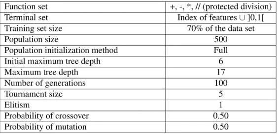
Function set +, -, *, // (protected division)

Terminal set Index of features ∪ ]0,1[

Training set size 70% of the data set

Population size 500

Population initialization method Full

Initial maximum tree depth 6

Maximum tree depth 17

Number of generations 100

Tournament size 5

Elitism 1

Probability of crossover 0.50

Probability of mutation 0.50

(39)

3.3 Algorithm

3.3.1 Elements of the M3GP algorithm

The initialization of our implementation of the M3GP is very similar to the one used in standard GP and specified in Genetic Programming: On the programming of computers by means of natural selection(1992) [3], and was made an attempt to be the same used in (L. Mu˜noz, 2015) [4]. In this sub-section, we will describe the elements of our approach when implementing the M3GP algorithm: we will describe how it is initialized, how the individuals are evaluated, how the individuals are selected and evolve, what is the function of the pruning GO, and how the elitism was implemented. In this sub-section, we may not give details about some parameters that were already mentioned in 3.2. We will mention some of the new genetic operators, but further details about them will only be given in 3.3.3. We should mention that the new mutation GOs are allegedly bad and were only implemented in order to test the behavior of M3GP when it’s given the chance to avoid using these operators.

Initialization: In order to search for more simple solutions first, each individual is created with only one branch at its root. This means that in the first generation, all in-dividuals have only one dimension. To promote diversity among the initial population, every individual is created using the Full method. In other words, the initial population would be the same in standard GP with the exception that the root node is a dummy node whose only purpose is to agregate the branches that represent each dimension. This dummy node is never changed by the genetic operators.

Evaluation: When an individual is created, it converts the training dataset into points in a Rnspace, where the centroid and covariance matrix of each class are then calculated. Using these two elements, when a sample from a dataset is given to the individual, the Ma-halanobis distance from the sample to each centroid is calculated, and the closest centroid is selected class as the predicted class. Another variation was made in this project. This variation used the Euclidean distance instead of the Mahalanobis distance. Other than this, the fitness function is equivalent. The individuals are evaluated using an accuracy-based fitness function. This kind of fitness function considers an individual superior to another if it has the highest accuracy. If they tie on accuracy, the smaller individual is preferred. The individuals could also be evaluated using a distance-based fitness function that tried to increase the distance between centroids while decreasing the distance that each sample has to their respective centroid. These fitness functions will be mentioned later in 3.3.2.

Selection for breeding: The parents of the next generation of individuals are selected by tournament. Each tournament receives the population and randomly selects five in-dividuals. From these individuals, the one with the highest fitness is the winner of the tournament, and a future parent.

(40)

Crossover: This implementation uses two crossover methods. Both methods receive two individuals. The first method (St-XO) randomly selects a node in each individual and swaps the nodes, just like the subtree crossover method proposed by Koza for the standard GP. The second method (Swap-dim) randomly selects a dimension in each in-dividual and swaps the dimensions. At the third stage of this project, a third crossover method (Swap3-dim) was implemented. This method randomly selects a dimension in each of three individuals and moves the first dimension to the second individual, the sec-ond dimension to the third individual and the third dimension to the first individual.

Mutation: This implementation contains three mutation methods. The first method (St-Mut) is the mutation used in standard GP. It randomly selects a node within the in-dividual and replaces the node with a new tree generated using the Grow method. The second method (Add-dim) adds a new dimension to the individual. This dimension is a new tree generated using Grow. The third method (Rem-dim) removes a randomly se-lected dimension from an individual with at least two dimensions. If the individual has one dimension and the third method is selected, the individual is returned unmodified. At the third stage of this project, four other mutation operators were implemented. One removed all dimensions except one and turns that dimension’s root node into a terminal node. Another randomly selects a dimension and turns its root node into a terminal node. The other two methods randomly select a node within an individual. One turns the node into a terminal node if it’s not terminal and if the node is terminal it’s replaced by a new tree, generated using Grow. The other operator turns the node into a terminal node. A more extensive description of these new mutation genetic operators is written in 3.3.3.

Pruning: Starting with the first dimension of the individual and ending with the last dimensions. This method evaluated the individual without one of its dimensions at a time. If its fitness improves with the removal of this dimensions, this dimensions is removed permanently. If the individuals have only one dimension, this method does nothing to the individual. Due to the high computational complexity of this operator, it is applied only to the best individual of each generation.

Elitism: Besides the pruned individual, the second best individual is always selected to move to the next generation without any modifications made.

Genetic Operator Selection: At the first stage of this project, the program would randomly select, with equal probability, either crossover or mutation. After this, it would randomly select a specific genetic operator of that category from those available. For the third stage of this project, the barrier between crossover and mutation was removed and initially each specific genetic operator has the same probability of being selected. Unlike before, this probability does not have a fixed value, it is meant to be able to increase or decrease according to its effect on the fitness of the individuals.

The evolution ends when the maximum number of generations is reached or when an individual has perfect accuracy on the training set. Until one of these conditions is

(41)

n Number of nodes of the individual d Number of dimension of the individual c Number of classes on the dataset s Number of samples on the training set

si Coordinates of the sample i on the output space

ccc Coordinates of the centroid i

cli Coordinates of the centroid of the labeled class for the sample i

Acc Overall accuracy of the individual

Table 3.3: Variables used in the fitness functions

met, the following steps will occur in a cycle: The individuals are evaluated using the chosen fitness function. They are then sorted from best to worst. The best individual is selected to be pruned and is added to the next generation, while the second best is selected through elitism. Until the next generation has 500 individuals, individuals are selected via tournament to be used in crossover or mutation. If the resulting individual from a genetic operation has a depth greater than 17, it is discarded.

3.3.2 Fitness Functions

As mentioned before, in this project we intend to replace an accuracy-based fitness function with a distance-based fitness function. To do that, we implemented and tested two distance-based fitness functions. Since these functions use the Euclidean distance, to have a fair point of comparison, we also implemented an accuracy-based fitness function that classifies a sample by associating it with the class of the closest centroid on the output space of the individual, using the Euclidean distance instead of the Mahalanobis distance. This function allows us to know if a distance-based fitness function has better results than an accuracy-based fitness function.

Here we describe each of the different fitness functions implemented. These functions use as variables the size and number of dimensions of the individual, the number of classes and samples on the training set, the coordinates of the samples on the output space, and the coordinates of the centroids of each class. These variables’ description can be seen in Table 3.3.

Sigmoid:

Sigmoid functions have a few properties that are very useful for our fitness functions. They are strictly crescent, return a value in ]0, 1[, and, for positive values, the growth never stops decreasing. This last part can be confirmed by deriving the sigmoid function. For positive values, the derivate is strictly decrescent and tends to 0. We decided to use this sigmoid function 3.1 because although all sigmoids have these properties, this sigmoid has a slower growth. From a x value onwards, the value obtained by S(x) will be 1. This