M
ASTER OF
S
CIENCE IN
E
CONOMICS
M
ASTER
’
S
F
INAL
W
ORK
D
ISSERTATION
T
HE
M
ACROECONOMIC
E
FFECTS OF
P
UBLIC
D
EBT
:
A
N
E
MPIRICAL
A
NALYSIS OF
M
OZAMBIQUE
Y
ASFIR
D
AUDO
I
BRAIMO
M
ASTER OF
S
CIENCE IN
E
CONOMICS
M
ASTER
’
S
F
INAL
W
ORK
D
ISSERTATION
T
HE
M
ACROECONOMIC
E
FFECTS OF
P
UBLIC
D
EBT
:
A
N
E
MPIRICAL
A
NALYSIS OF
M
OZAMBIQUE
Y
ASFIR
D
AUDO
I
BRAIMO
S
UPERVISOR:
A
NTÓNIOM
ANUELP
EDROA
FONSOAbstract
Public debt has been rising markedly over the years, which suggests an increase in public expenditure financed by debt instead of taxation. There is no consensus on the economic implications of borrowing to finance public expenditure. This dissertation empirically investigates the macroeconomic effects of public debt for the case of Mozambique over the period of 2000Q1-2016Q4. Vector Autoregression (VAR) model are used to assess these effects through impulse response functions and variance decomposition. We conclude that debt service variables have much more negative effects on this economy than debt variables. Debt variables over the period of this study had no significant impact on the real output and the debt service component depressed the real output, increased the general price level and accounted for depreciation on the domestic currency.
Keywords: External Debt, Domestic Debt, External Debt Service, Domestic Debt
Service, Total Debt, Total Debt Service, Exchange Rate, Lending Rate, Treasury Bills Rate, Consumer Price Index, Impulse Response, Variance Decomposition, Vector Autogression Model
Acknowledgments
I would like to dedicate this work to my children, Tahir and Rayhan, and many apologies for my absence during this course.
I would like to thank the Instituto de Estudos Sociais e Economicos (IESE), in Mozambique, for the scholarship.
I also thank my supervisor, Professor António Afonso, for the careful and incredible support in all phases of this dissertation.
At last, thank my colleagues from the master in Economics and from Monetary and Financial Economics.
Contents Abstract ... ii Acknowledgments ... iii Contents... iv List of Figures ... v List of Tables ... v 1. Introduction ... 1 2. Literature Review ... 4 2.1 Theoretical Literature ... 4 2.2 Empirical Literature ... 8
3. Methodology, Data and Model Estimation ... 11
3.1. Analytical Framework ... 11
3.2. Data Description ... 15
3.3. Unit Root Test ... 16
3.4. Model Specification ... 17
3.5. Lag Selection, Residual and Stability test ... 18
4. Estimation and Empirical Results ... 19
4.1. Estimation Results ... 19 4.2. Model 1 ... 20 4.2.1. Impulse Response ... 20 4.2.2. Variance Decomposition ... 21 4.3. Model 2 ... 23 4.3.1. Impulse Response ... 23 4.3.2. Variance Decomposition ... 24 4.4. Model 3 ... 26 4.4.1. Impulse Response ... 26 4.4.2. Variance Decomposition ... 27 4.5. Model 4 ... 29 4.5.1. Impulse response ... 29 4.5.2. Variance Decomposition ... 30 4.6. Model 5 ... 31 4.6.1. Impulse response ... 31 4.6.2. Variance Decomposition ... 33
4.7. Model 6 ... 34 4.7.1. Impulse response ... 34 4.7.2. Variance Decomposition ... 35 5. Conclusions ... 37 References ... 40 APPENDIX ... 44 List of Figures Figure 1: Effects of positive shocks in ED on L_RATE, T_BILL, RGDP, EXC and CPI ... 21
Figure 2: Effects of positive shocks in DD on EXC, L_RATE, T_BILL, RGDP, and CPI ... 24
Figure 3: Effects of positive shocks in EDS on L_RATE, T_BILL, EXC, RGDP, and CPI ... 27
Figure 4: Effects of positive shocks in DDS on EXC, L_RATE, T_BILL, RGDP, and CPI ... 30
Figure 5: Effects of positive shocks in TD on L_RATE, T_BILL, EXC, RGDP, and CPI ... 32
Figure 6: Effects of positive shocks in TDS on EXC, T_BILL, L_RATE, RGDP, and CPI ... 35
List of Tables Table 1: Variance Decomposition (%) ... 22
Table 2: Variance Decomposition (%) ... 25
Table 3: Variance Decomposition (%) ... 28
Table 4: Variance decomposition (%) ... 31
Table 5: Variance Decomposition (%) ... 33
1. Introduction
Economic growth and price stability are the main macroeconomic goals in any economy. To reach this, many economies have been increasing government expenditure through the combination of taxation and issuing public debt. Despite this, in many countries, public debt has been rising markedly over the years, which seems to be due to an increase in public expenditure financed by debt instead of taxation. In the case of Mozambique, as showed by Castel-Branco (2014) and Massarongo (2016) public debt has been growing rapidly, and since 2006 its composition has changed from concessional debt to commercial debt, which is unsustainable given the economic structure of this country, high-interest rate and short maturity of the debt.
Public debt is not a new issue in economic literature, but recently with the increase in the more indebted countries, those concerns became a hot topic in this literature. However, despite the existence of a vast set of theoretical and empirical works investigating this issue, there is no consensus on the macroeconomic implications of borrowing to finance public expenditure. It means that it is not clear that raising public debt will increase economic growth and improve other macroeconomic indicators.
Despite the contribution of many studies on the issue of public debt, there is few theoretical and empirical discussion considering public debt separately as external debt and domestic debt. Therefore, it is important to analyse the effects of external and domestic debt separately because they provide different sources of vulnerability, mainly for developing countries with non-developed capital markets and high currency volatility. On one hand, in these countries, the concerns with external debt can be the volatility of the real exchange rate,
which can be a source of a negative economic implication for the economy. On the other hand, the short maturity and high-interest rate associated with domestic debt might be a risk for debt explosions (Panizza, 2008).
Inspired by the few empirical studies of this subject, and the fact that the effects of public debt vary according to the specific economic structures and debt composition, this dissertation empirically investigates the macroeconomic effects of public debt on real output, price level, exchange rate, treasury bills rate and lending rate in Mozambique over the period of 2000Q1–2016Q4. Public debt effects are considered separately and in aggregate form, namely: external debt, domestic debt, external debt service, domestic debt service, total debt and total debt service. The empirical assessment is conducted through a Vector Autoregression (VAR) model, which according to Luetkepohl (2005) has proven to be useful for describing the dynamic behaviour of economic time series. The results are estimated from the structural analysis of VAR, namely: impulse response functions and variance decomposition. The application of this econometric model is an innovation in empirical literature of public debt in Mozambique, given scarce empirical studies on this subject.
The most relevant findings of this dissertation can be summarized as follows. External and total debt (i) have a positive effect on real output during few quarters (3 quarters) but not in the long-run; (ii) have an ambiguous result on price level and we cannot conclude about the inflationary tendency; (iii) lead to an appreciation of domestic currency in the short-run and a depreciation of currency in the long-run and (iv) in the short-run do not impact significantly on the interest rate variables (treasury bills rate and lending rate).
On the other hand, domestic debt (i) has a negative effect on real output during all periods; (ii) has a positive effect on price level in the short-run and recovery in the long-run;
(iii) leads to an appreciation of the domestic currency in the short-run and a depreciation of
the domestic currency in the long-run and (iv) in the short-run does not have significant impact on the interest rate variables, but in the long-run has a significant contribution to the treasury bills rate and consequently impact on the lending rate.
Further, the debt service variables, as external, domestic and total debt service; (i) have a strong negative effect on the real output; (ii) lead to a depreciation of the domestic currency against the US dollar; (iii) do not impact significantly on both treasury bills rate and lending rate in the short-run, but have a positive effect on both variables, mainly on the lending rate, in the long-run. The opposite was found for the domestic debt service, which has a positive effect and becomes significant in the long-run; (iv) debt service variables have a positive effect on the price level, which suggests the existence of inflationary episodes.
Overall, the empirical analysis shows that debt service variables have deeply negative macroeconomic effects compared to debt variables. In addition, the estimated models show a significant role of the exchange rate in this economy, which shows its vulnerability with exchange rate fluctuation.
The remaining part of this paper is structured as follows. Section two reviews the theoretical and empirical literature about public debt issues. Section three presents the methodology, data, model estimation and development of the analytical framework. Section four provides the empirical estimation and discusses the results. Section five presents the main conclusion of this dissertation.
2. Literature Review
2.1 Theoretical Literature
Issuing public debt is considered an important mechanism to finance government projects and hence stimulate aggregate demand towards full employment. In contrast, some scholars argue that the use of taxation is an appropriate way to finance government expenditure.
The theoretical literature which investigates public debt and economic growth is quite rich and diverse. According to Modigliani (1961), Diamond (1965), Saint-Paul (1992) and Aizenman et al. (2007), there is a negative relationship between government debt and economic growth. On one hand, there exist crowding-out effects on private investment because of higher real interest rate across the financial market, given the higher demand for credit created in this market, and the relatively inefficient use of resources by the government. On the other hand, public debt is considered an intergenerational burden because it takes a smaller stock of capital for future generations.
Buchanan (1958) raised the question of who pays for public debt and when do they pay. This question was raised by the concerns over government expenditure financed by debt instead of taxation because these loans would not be used to finance capital investments. Therefore, Buchanan (1958) argues in that financing public expenditure by issuing debt will transfer the burden to future generations because the government will end up raising taxes to pay the debt.
Barro (1974) argues that fiscal stimulus is inefficient to achieve economic growth. This argument is based on the Ricardian equivalence theory, where an increase in
government spending financed by debt is offset by an increase in private savings because the economic agents will anticipate a future increase in taxes. Additionally, Elmendorf & Mankiw (1999) advocate that in the short-run output will respond positively to public debt, and because of the crowding-out effect, in the long run, the output will decrease.
A literature survey by Sardoni (2013) makes a distinction between mainstream and Keynesian approaches. The mainstream view often treats public debt as private debt and consequently, at some point in time, the government must raise the taxes to meet its debt obligations. As a result, private demand will decrease and the positive effect on growth induced by high public expenditure is neutralized by the negative effect of taxes. The standard Keynesian models describe the opposite, where public debt is considered necessary to ensure a high level of aggregate demand and keep the economy towards full employment. Moreover, it is important to take account of the fundamental distinction made by Keynesian approaches between the current and capital expenditure. For Keynes, issuing public debt to finance expenditure in capital can positively affect economic growth.
Despite the existence of some criticism over the macroeconomic impact of public debt, recent studies have argued that in a context of increasing fiscal imbalances, moderate levels of government debt can induce economic growth (Afonso & Jalles, 2016).
Focusing on developing countries, Afonso & Jalles (2015), state the presence of a large government debt-to-GDP ratio has a strong negative impact on private investment in several ways. First, it reduces available funds for private investment, where a higher debt service payment is involved. Second, it reduces incentives for private investment because of the anticipated taxes on future income and returns on investment.
Based on the Laffer curve theory, Mbate (2013) concludes that there exists a non-linear relationship between public debt and economic growth. According to this theory, an initial level of domestic debt accelerates economic growth through resources for financing budget deficits. However, with a continuous increase in the debt stock, the economy experiences a debt overhang and economic growth begins to decline thereafter. This drop is attributed to a high debt servicing costs, which will reduce the availability of resources for productive investments. In addition, debt issuance may trigger a rise in interest rates, and consequently, raise the cost of borrowing for household consumption and capital accumulation. Moreover, Mbate (2013) reports that a large debt stock creates an atmosphere of uncertainty in the economy related to the kind of policies and actions that government may adopt to pay its debt. Such policies may include increases in tax rates, which may lower investment and force investors to either shift their investment portfolios to fewer indebted countries or hold back on their investment projects.
However, there are just a few theoretical discussions considering external and domestic debt separately. In the case of developing countries, with non-developed capital markets and high currency volatility, this separation is important because the effect of both kinds of debt on the economy is different. For instance, Emmanuel (2012) states that a high level of external debt will reduce the availability of funds for private investment because of payments of external debt service. Mehl & Reynaud (2010) consider that domestic debt has short-maturity and expose the government to a high probability of default. Reinhart & Rogoff (2008) show that the accumulation of a large domestic debt is often at the roots of external debt crises and large inflationary episodes.
Another strand of literature postulates that excessive issuance of domestic debt crowds out private sector credit, especially in countries where national savings are low and less developed financial markets. This occurs because the excessive use of domestic debt absorbs funds in the banking system, limiting the availability of resources for the private sector (Mbate, 2013).
According to Panizza (2008) what matters is not whether the debt is internal or external because the source of vulnerabilities is currency and maturity mismatches. This mismatch with the volatility of the real exchange rate, that characterizes most of developing countries, increases the volatility of GDP growth and capital flows and the risk of sudden debt explosions, which often put these countries in a vulnerable situation. Additionally, countries that are switching from external to domestic debt could be trading a currency mismatch for a maturity mismatch. Alternatively, the switch to domestic borrowing could lead to pressure investors and banks to absorb too much public debt and this may have a negative effect on financial stability.
Based on the concept of extractive economy1, Castel-Branco (2010, 2013, 2014)
examines the multiplier effect of public debt given certain economics structures. Thus, the expected multiplier effect of public debt will be determined through the linkage between the country’s economic structures and the fiscal and monetary policy.
According to Castel-Branco (2011, 2017), there is higher social and economic cost of financing government expenditure through public debt. Firstly, the debt service puts
1 The concept of extractive economy is characterized by high growth rates and stable macroeconomic indicators, but with a
fragile economic structure where much of economic growth is concentrated in large projects with weak links with the rest of the economy, and which has most of the services and investments adjacent, so the economy remains fragile, vulnerable to external shocks, with a low capacity to reduce poverty (Castel-Branco, 2010, 2013, 2014).
pressure on the available resources, the structure of public expenditure and makes government unable to pursue broader social and economic policies. Secondly, it will create competition for financial resources between the state and private sector, which will increase the cost of financial capital and consequently, the investment to diversify production base becomes expensive and undermines the conditions for economic transformation.Thirdly, the financial sector may concentrate their activity in financial transactions and speculation with financial assets instead of financing productive activities. Fourthly, the tendency for public spending focuses on projects with high financial returns instead to finance the development of a national production capacity. In the case of Mozambique, public debt has been used to finance large-scale of infrastructure, because it is the main source of economic growth and guarantee sufficient rates of return to sustain the debt costs. However, it will end up reproducing a concentrated and disjointed system of accumulation that weakens the economy and limits the multiplier effect of public debt.
2.2 Empirical Literature
Despite the wide theoretical literature on public debt, empirical studies on this issue have been focusing mainly on advanced economies (Afonso & Jalles, 2016). In developing countries, and specifically in Mozambique such research remains scarce and the absence of well-organized data might be one of the main reasons.
Afonso & Alves (2015) examine the effect of government debt on real per capita GDP growth for annual and 5-year average growth rates through panel data techniques for 14 European countries from 1970 to 2012. This study concludes that (i) government debt has a negative effect on economic growth, both in the short and long-term, (ii) debt service has a
much more negative effect on economic performance than debt and (iii) there is an inverted U-shape relationship between the debt ratio and economic growth.
Checherita & Rother (2010), investigate the average impact of government debt-to-GDP ratio on per-capita debt-to-GDP growth in 12 Euro area countries over a period of 40 years starting in 1970. The study used a growth model and a conditional convergence equation. The channels through which government debt is found to have an impact on the economic growth rate are private saving, public investment, total factor productivity and sovereign long-term nominal and real interest rates. The paper also found the existence of a non-linear impact of public debt on growth with a turning point beyond 90-100% of GDP, which the government debt-to-GDP ratio has an adverse effect on long-term growth. Additionally, the confidence intervals for the debt turning point suggest that the negative growth effect of high debt may start already from levels of around 70-80% of GDP.
Schclarek (2004), investigates the relationship between public debt and per capita GDP growth in 24 advanced countries and 59 developing countries using panel data for the period 1970-2002. In advanced countries, the paper does not find any robust evidence suggesting that higher public debt levels are not necessarily associated with lower GDP growth rates. For developing countries, it finds always a negative and significant relationship between debt and growth.
Additionally, Woo & Kumar (2015) study empirically the long-run effects of initial high public debt on economic growth in a large panel data of advanced and emerging countries from 1970-2008 based on growth regressions and growth accounting techniques. Through the estimation of cross-country OLS regressions and GMM, they found a robust inverse relationship between initial debt and subsequent growth. It means that there is some
evidence of non-linearity, with only above 90% of debt-to-GDP ratios having a significant negative effect on growth.
Reinhart & Rogoff (2010) investigate the relationship between government debt and economic growth through the evidence of 20 advanced countries and emerging countries from 1970–2009. The findings for advanced countries showed no clear relationship between debt and economic growth until public debt reaches a threshold of 90%. For developing countries, it was found that an external debt level over 60% and further external debt levels that exceed 90% reduce markedly economic growth. Inflation tendency becomes significantly higher only for countries with external debt over 90%. Therefore, this study evidences the relevance of debt threshold analysis on economic growth and suggest that public debt could not be a terrible thing at all.
Focusing on developing countries and narrowly on external public debt, Pattillo et al. (2002) found a non-linear impact of government debt on economic growth and a negative impact of external debt on per-capita GDP growth for net present value of debt levels above 35-40% of GDP using a large panel dataset of 93 countries over 1969-1998. In the same view, Clements et al. (2003) explore the relationship between government debt and growth for a panel data of 55 low-income countries during the period of 1970-1999. They found the negative effect of external public debt on growth when the value of this debt reaches about 20-25% of GDP. Furthermore, Clements et al. (2003) emphasize that external debt can crowd-out private investment or alter the composition of public spending. High debt service can raise the interest rate through increased budget deficits. To finance these budget deficits, the government may crowd-out credit available to private investment causing a decrease in economic growth.
Mbate (2013) studied the impact of domestic public debt on economic growth and private sector credit in Sub-Saharan African countries. The result shows the existence of a non-linear relationship between domestic debt and economic growth. For this study, a domestic debt level above 11.4 % of GDP represents a risk of triggering domestic debt distress and undermining a country’s fiscal and debt sustainability position. Further, the evidence about domestic debt structure showed a short maturity and concentration of this kind of debt in the portfolios of the banking sector.
In addition, Emmanuel (2012) assess the impact of public debt on economic growth in Nigeria, where he found a negative and quite significant impact of public debt on economic growth in the long-run, and a positive effect in the short-run. Furthermore, Ekperiware & Oladeji (2012) examine the effect of external debt relief on economic growth in Nigeria between 1975 and 2005. They found a structural break in the relationship between economic growth and external debt, where the external debt relief made more resources available for economic growth. In the case of Kenya, Putuoni & Mutuku (2013), found a positive and significant relationship between domestic debt and economic growth, and recommend an expansion of domestic debt markets to transfers resources to finance productive investments.
3. Methodology, Data and Model Estimation
3.1. Analytical Framework
To support the empirical analysis this dissertation is developed an analytical framework based on research findings from Castel-Branco (2010, 2014) and Massarongo
(2016), who consider the importance of the Mozambique economic structure, public debt and debt service composition for evaluating the economic impact of public debt. Therefore, this framework seeks to explain the transmission mechanism through which debt variables of the model can be channelled to the economy.
Castel-Branco (2010) presents three main characteristics, which describe the Mozambican economy, and this will help to understand how public debt will affect the economy. First, there is a concentration in production and exports in primary goods, with less add value and in some cases only with primary industrial transformation. As a result, the revenues and the expansion of the economy are highly dependent on the increase of exports of this kind of product, which depends on the dynamics of the international markets of commodities. Second, there exists a chronic dependence on imports of basic consumer goods and raw material for many production sectors. Third, there is a disarticulation of productions activities with the limited linkage between sectors and activities.
Besides the economic structure, the composition of public debt and debt service also matters for the evaluation of the macroeconomic effects of debt variables. It can be supported by the evidence presented by Massarongo (2016), where changes in debt composition in Mozambique since 2005 until 2016, from concessional to commercial debt, both external and domestic, had strong effects on the economy associated with higher interest rates and low maturity in commercial debt. According to this author, falls in donor’s aid to the government budget increased domestic debt, because the government started to have less short-term cash flows. Indeed, this type of debt becomes expensive because of the associated debt service.
Given the economic structure and the debt composition described above, it is predicted that the transmission of the debt effects in the economy is channelled through
exchange rate and interest rate variables. On one hand, because the exchange rate channel is associated with external debt and debt service and given that this economy is a net importer, the depreciation in domestic currency has a significant impact on the economy. On the other hand, the domestic debt and debt service will affect the interest rate variables, namely: treasury bills rate and lending rate because of the competition on financial resources between government and private agents. To accurately assess the effect of debt and debt service variables, we combine the disaggregate and aggregate analysis because it is expected that it is channelled and felt in a different way.
Regarding the external debt, the transmission mechanism is channelled mainly through the exchange rate and output. Because an external debt shock means an inflow of financial resources into the economy, which would temporarily increase the country’s reserve in external currency. This amount can be temporarily used by the Central Bank to stabilize the exchange rate through the sterilization mechanism in the inter-bank market. Consequently, the stability of the exchange rate will contribute to mitigating the inflationary tendency, given that the Mozambican economy is a net importer of basic consumer goods and raw materials. Another effect will be directly felt in output through the increase in government expenditure and thereby stimulate the economic activities toward economic growth. The interest rate variables are probably expected not to be influenced by the external debt for two reasons: (i) the government is being financed with external resources, which reduces the domestic competition in financial resources and (ii) the stability in price level influenced by stability in exchange rate, probably will likely contribute to control potential Central Bank intervention of raising interest rate to control inflationary tendency.
For external debt service, despite the same transmission mechanism with external debt, the effect on the economy will differ. In this case, external debt service represents fixed debt obligations, which government must repay. Consequently, this payment means an outflow of resources in external currency and less availability of the resource to finance other government projects. In addition, this payment will increase the exchange rate, which will translate into depreciation in domestic currency. Given the economic structure of Mozambique, the depreciation of the currency will create inflationary tendency through the importation of consumer goods and raw materials. To tackle the inflationary tendency the Central Bank will react raising the interest rate. The output will be affected from both sides. On one side, there will be less availability of resources because of the outflow of the resource. On the other side, there will also be an increase in the cost of capital and expenses paid for import of raw materials.
Further, the effect of issuing domestic debt can be spread through interest rate variables and output. This kind of debt is issued by the government through the sale of treasury bills with a given interest rate. Given the limited domestic financial resources, the continuous use of domestic debt by government probably will increase the treasury bills interest rate. Consequently, due to lag effects, the lending rate will also increase. As a result, capital becomes more expensive which will affect economic activity and the level of output. Moreover, the capacity of the private sector to finance its investment projects will decrease. However, the output will be directly affected by the limited availability of resources and the high cost of capital. There will be no expectation on inflationary tendency given the increase in domestic debt because the increase in interest rate will affect inflation.
The effect of domestic debt service will also spread into the economy through the interest rates and output channels. Domestic debt service is characterized by high-interest rate and short maturity, and consequently, represents a significant cost for the economy. As a result, the payment of this obligation will reduce the available resources in the economy and probably output will fall. There is a tendency for an increase in the treasury bills rate if the government rolls over the debt to pay old debt. Consequently, the lending rate will be affected by the increase in the treasury bills rate.
3.2. Data Description
The data used to estimate the model consists of quarterly time-series ranging from 2000Q1 to 2016Q4. Given that some data are not available on a quarterly basis, interpolation methods calculated by Eviews was used keeping the original series behaviour. Overall, we will use eleven variables, namely: Real Gross Domestic Product (𝑅𝐺𝐷𝑃), Consumer Price Index (𝐶𝑃𝐼), average three months of Prime Lending Rate (𝐿_𝑅𝐴𝑇𝐸), average yield on 91-day Treasury Bills rate (𝑇_𝐵𝐼𝐿𝐿), Nominal Exchange Rate (𝐸𝑋𝐶) in average quarterly of national currency per US Dollar, Public Domestic Debt (𝐷𝐷), Public External Debt (𝐸𝐷), Total Debt (𝑇𝐷), Domestic Debt Service (𝐷𝐷𝑆), External Debt Service (𝐸𝐷𝑆) and Total Debt Service (𝑇𝐷𝑆).
𝑅𝐺𝐷𝑃, 𝐶𝑃𝐼, 𝐿_𝑅𝐴𝑇𝐸, 𝑇_𝐵𝐼𝐿𝐿 and 𝐸𝑋𝐶 are used in the model to capture the effects of a shock on public debt and debt service in these variables. Specifically, 𝑅𝐺𝐷𝑃 is employed to capture the effect on output. The 𝐶𝑃𝐼 is used as a proxy of the general price level, given that measure changes in the prices of goods and services purchased by households. Both data were taken from the web page of the National Institute of Statistics from Mozambique. The
𝐿_𝑅𝐴𝑇𝐸 and 𝑇_𝐵𝐼𝐿𝐿 is used as a proxy for the interest rate in the economy. The 𝐸𝑋𝐶 is used to capture the relation of national economy with the world. Additionally, the increase in nominal 𝐸𝑋𝐶 is equivalent to the depreciation in domestic currency against the US Dollar. The last three variables were taken from the International Monetary Fund (IMF) database but according to the IMF description, this data was produced by the Central Bank of Mozambique. The debt variables namely: 𝐷𝐷, 𝐸𝐷, 𝐷𝐷𝑆, 𝐸𝐷𝑆 were obtained from the government of Mozambique, specifically the Ministry of Economy and Finance. The 𝑇𝐷 and 𝑇𝐷𝑆 were calculated by the author through the sum of the respective domestic and external component of the debt and debt service.
In addition, the variables employed in the model were transformed in natural logarithms, except on the 𝑇_𝐵𝐼𝐿𝐿 and 𝐿_𝑅𝐴𝑇𝐸, because these variables were presented in percentage. One advantage of converting data in logarithms is to control for possible heteroscedasticity problems in the residuals terms. Further, to verify the distribution of data being used for empirical analysis, some descriptive analyses were employed. Table A1 in the appendix shows the results of the descriptive statistical analysis of the data.
3.3. Unit Root Test
Examine the behaviour of data is an important step before the model specification. One of the main characteristics in many economic data is trending, as a result, the presence of unit root is inevitable. In other words, data with unit root is non-stationary. However, this kind of data is not suitable for the model and can produce some dubious results. According to Lutkepohl (2005), traditionally VAR models are designed for stationary variables without time trends. However, to analyse the behaviour of data it is important to employ the unit root
test. As suggested by Said & Dickey (1984), the non-stationary time series can be transformed into a stationary one. Specifically, two kinds of unit root tests were carried out, namely the Augmented Dickey-Fuller (ADF) and the Philip-Perron (P-P) testes. Firstly, these tests were employed at the level, but as predicted, they showed non-stationary behaviour at 5% critical value. Finally, following Said and Dickey (1984), the data was transformed into a stationary (constant mean and variance) through the first difference method. The results of those tests are summarized in table A2 and A3, respectively of the appendix.
3.4. Model Specification
The unrestricted Vector Autoregression (VAR) model will be adopted to assess the macroeconomic effects of public debt in Mozambique. This model was advocated for macroeconometric analysis and becames popular by Sims (1980). According to Luetkepohl (2005), the VAR model has proven to be useful for describing the dynamic behaviour of economic time series.
Further, the structural analysis through the impulse response function and the variance decomposition are important tools of this kind of model. The impulse response function traces the effects of one standard deviation positive shocks of one of the innovations on current and future values of the endogenous variables. This function allows for seeing a time and dimensional impact of a shock or innovation in public debt variables on a selected macroeconomic variable. While the variance decomposition quantifies the contribution of the shocks to a variation on another variable. However, the variance decomposition was conducted to quantify the portion of variation in the selected macroeconomic variables due to shock in public debt and debt service variables.
The VAR model is specified in the following form:
𝑌𝑡= 𝐴1𝑌𝑡−1+ 𝐴2𝑌𝑡−2+ ⋯ + 𝐴𝑘𝑌𝑡−𝑘+ 𝜇𝑡 (1) 𝑌𝑡= [𝐿𝑅𝑡, 𝑇𝐵𝐼𝐿𝐿𝑡, 𝐸𝐷𝑡, 𝐸𝐷𝑆𝑡, 𝐷𝐷𝑡, 𝐷𝐷𝑆𝑡,𝑇𝐷𝑡, 𝑇𝐷𝑆𝑡, 𝑅𝐺𝐷𝑃𝑡, 𝐸𝑋𝐶𝑡, 𝐶𝑃𝐼𝑡] (2) where 𝐴 is a 𝑛𝑥𝑛 matrix of coefficients, 𝑌𝑡 are the endogenous variables, and 𝜇𝑡 is an
(𝑛𝑥1) matrix representing unobservable zero mean white noise error, where it must be serially uncorrelated. In a VAR model, all variables are treated as endogenous and regressed on its own lags. The advantage of this model is the spread of the dynamic transmission of shocks in any variable over time, for instance, how the shocks in public debt at time 𝑡 will affect the macroeconomic variables at time 𝑡 + 1. Specifically, for this dissertation six VAR models will be estimated.
The order of the variables in VAR is fundamental. So, in each estimated model the first variable was ordered assuming that its response to all other variables is not instantaneous. Output and price level responds contemporaneously to all other endogenous variables.
3.5. Lag Selection, Residual and Stability test
The optimal lag length test was employed for each model to determine the optimal lag to estimate the model. However, for each model, the result of the test suggested 5 lags as the optimal lag length. As a result, the VAR model was estimated with 5 lags. The results of this test for each model are presented in the tables A4 (model 1), A7 (model 2), A10 (model 3), A13 (model 4), A16 (model 5), and A19 (model 6) in the Appendix.
The residual test, namely: the autocorrelation LM test and heteroscedasticity test and the model stability test through the Roots of Characteristic Polynomial were employed. The
residual LM test was employed to check the whiteness of the residuals, which means whether exist or not the presence of serial correlation in the disturbance term of the model. According to the results of this test, the null hypothesis (no serial correlation) cannot be rejected at a significance level of 5%, which implies no serial correlation. The result of the stability test of the VAR model through Roots of Characteristic Polynomial shows that none of the roots of the model lies outside the circle, which implies that the VAR model satisfies the stability condition. In this case, the transformation of all variables of the model to first difference was important to guarantee the stability of the model. The heteroscedasticity test was also conducted, and it shows that there is no evidence of heteroscedasticity at 5% significance level. The results of all these tests are presented in the tables A5 and A6 (model 1), A8 and A9 (model 2), A11 and A12 (model 3), A14 and A15 (model 4), A17 and A18 (model 5), A20 and A21 (model 6) in the Appendix.
4. Estimation and Empirical Results
4.1. Estimation Results
The main results of the models are produced through the structural analysis of the VAR model, namely: the impulse response functions and the variance decomposition. However, an impulse response analysis of RGDP, CPI, EXC, L_RATE, and T_BILL to innovations on the public debt and debt service variables for 10 quarters was carried out. The same analysis was employed to the variance decomposition and the results are presented for four periods, namely 1st, 4th, 8th and 10th quarter.
4.2. Model 1
4.2.1. Impulse Response
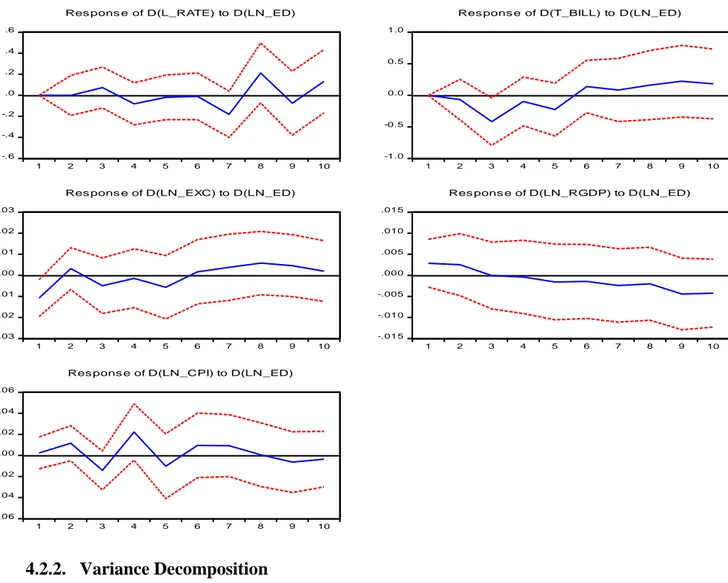
Figure 1 describes the repercussions of one standard deviation positive shocks of external debt, after estimating the following model:
𝑌𝑡= [𝐿𝑅𝑡, 𝑇𝐵𝐼𝐿𝐿𝑡, 𝐸𝐷𝑡, 𝐸𝑋𝐶𝑡, 𝑅𝐺𝐷𝑃𝑡, 𝐶𝑃𝐼𝑡] (3) The results suggest that real output declines steadily following the shock which erodes after 3 quarters. It means that public external borrowing only has a few positive effects on real output in the short-run, but not in the long-run. The results show that after external debt shock, during 6 quarters, the exchange rate responds negatively which means an appreciation of the domestic currency, but after this quarter the domestic currency displays a slight depreciation. The behaviour of the exchange rate corroborates with our analytical framework, which predicts the use of the sterilization mechanism by the Central Bank to stabilize the exchange rate. Treasury bills rate responds negatively during 6 quarter, and after that is positively affected by the shock. This reaction can be explained by the few demands for domestic resources by the government. Lending rate, in general, during 7 quarters responds negatively to an external debt shock, but after 8 quarters starts to present fluctuations between positive and negative reactions. Overall, in the short-run external debt does not affect both interest rate variables because the government will be using external resources. Finally, the result shows that after the external debt shock, the price level shows an ambiguous result. During 8 quarters the price level was characterized by fluctuations between the positive and negative reaction to a shock but ends with a negative reaction. From
this result, we cannot conclude about the inflationary tendency created by the external debt shock.
Figure 1: Effects of positive shocks in ED on L_RATE, T_BILL, RGDP, EXC and CPI
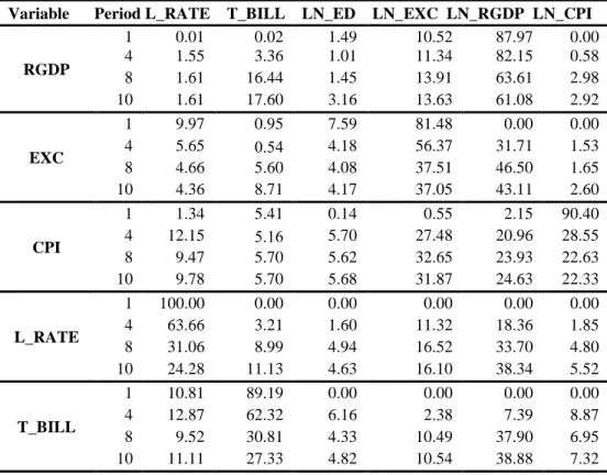
4.2.2. Variance Decomposition
Table 1 provides the results of the variance decomposition in percentage, to evaluate the proportion of the variation of RGDP, CPI, EXC, LR and T_BILL rate to a shock or innovation in all endogenous variables. External debt shock has a weak contribution (less than 8%) on variations of the selected variables. It means that external public debt does not
-.6 -.4 -.2 .0 .2 .4 .6 1 2 3 4 5 6 7 8 9 10
Res pons e of D(L_RATE) to D(LN_ED)
-1.0 -0.5 0.0 0.5 1.0 1 2 3 4 5 6 7 8 9 10
Res pons e of D(T_BILL) to D(LN_ED)
-.03 -.02 -.01 .00 .01 .02 .03 1 2 3 4 5 6 7 8 9 10
Res pons e of D(LN_EXC) to D(LN_ED)
-.015 -.010 -.005 .000 .005 .010 .015 1 2 3 4 5 6 7 8 9 10
Res pons e of D(LN_RGDP) to D(LN_ED)
-.06 -.04 -.02 .00 .02 .04 .06 1 2 3 4 5 6 7 8 9 10
Res pons e of D(LN_CPI) to D(LN_ED)
account significantly on variations of those macroeconomic variables. Despite, the weak effect of external debt, the results show a significant contribution of the exchange rate on the variation of most endogenous variables, except on the treasury bills rate. This result displays the vulnerability of this economy to exchange rate fluctuations. For instance, as predicted by the framework, through the economic structure of Mozambique, there is a significant weight of exchange rate in a variation of the general price level, which can support the inflationary tendency through this channel. Another important point to raise is the significant contribution of real output on variation in the endogenous variables of the model.
Table 1: Variance Decomposition (%)
Variable Period L_RATE T_BILL LN_ED LN_EXC LN_RGDP LN_CPI
RGDP 1 0.01 0.02 1.49 10.52 87.97 0.00 4 1.55 3.36 1.01 11.34 82.15 0.58 8 1.61 16.44 1.45 13.91 63.61 2.98 10 1.61 17.60 3.16 13.63 61.08 2.92 EXC 1 9.97 0.95 7.59 81.48 0.00 0.00 4 5.65 0.54 4.18 56.37 31.71 1.53 8 4.66 5.60 4.08 37.51 46.50 1.65 10 4.36 8.71 4.17 37.05 43.11 2.60 CPI 1 1.34 5.41 0.14 0.55 2.15 90.40 4 12.15 5.16 5.70 27.48 20.96 28.55 8 9.47 5.70 5.62 32.65 23.93 22.63 10 9.78 5.70 5.68 31.87 24.63 22.33 L_RATE 1 100.00 0.00 0.00 0.00 0.00 0.00 4 63.66 3.21 1.60 11.32 18.36 1.85 8 31.06 8.99 4.94 16.52 33.70 4.80 10 24.28 11.13 4.63 16.10 38.34 5.52 T_BILL 1 10.81 89.19 0.00 0.00 0.00 0.00 4 12.87 62.32 6.16 2.38 7.39 8.87 8 9.52 30.81 4.33 10.49 37.90 6.95 10 11.11 27.33 4.82 10.54 38.88 7.32
4.3. Model 2
4.3.1. Impulse Response
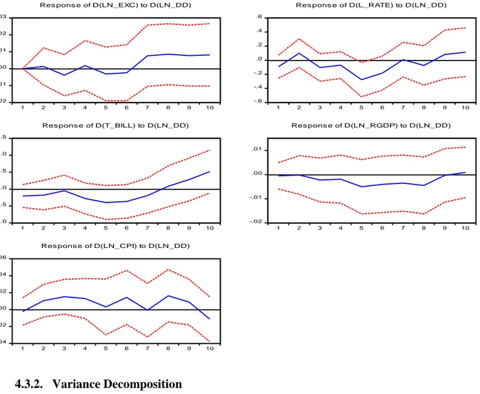
Figure 2 shows the impulse response function to a domestic debt shock, after estimating the following model:
𝑌𝑡= [𝐸𝑋𝐶𝑡, 𝐷𝐷𝑡, 𝐿𝑅𝑡, 𝑇𝐵𝐼𝐿𝐿𝑡, 𝑅𝐺𝐷𝑃𝑡, 𝐶𝑃𝐼𝑡] (4) Similarly, to model 1, the results show that real output did not respond to innovation on domestic debt until 9 quarters. This result follows our prediction from the analytical framework and some literature that domestic debt will reduce the available resources in the economy. After the domestic debt shock, treasury bills rate responds negatively during 8 quarters and becomes positive. Lending rate reacts positively, but this effect is only felt during 1 quarter and the following 6 quarters responds negatively to a domestic debt shock. After 9 quarters, the lending rate presents a positive reaction. This result suggests that both interest rate variables, in the short run, did not respond to innovation on domestic debt. However, in the long run with the successive issuing of domestic debt, treasury bills rate will be positively affected and consequently, the effect will stress the lending rate to a positive reaction to the shock. The response of the exchange rate becomes significant after 6 quarters with a positive reaction to a domestic debt shock. Finally, the results show that after a domestic debt shock, the general price level responds positively during 9 quarters and becomes negative from 10 quarters. This evidence suggests that the issuing of domestic debt tends to create an inflationary tendency.
Figure 2: Effects of positive shocks in DD on EXC, L_RATE, T_BILL, RGDP, and CPI
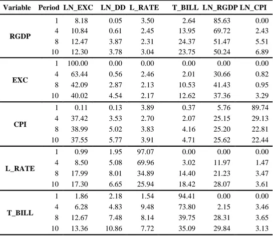
4.3.2. Variance Decomposition
Table 2 shows the results of the variance decomposition in percentage, to assess the proportion of the variation on RGDP, CPI, EXC, LR and T_BILL rate to a shock or innovation in all endogenous variables. The results indicate that variation in domestic debt accounts for significant contribution to the treasury bills rate (10.86% in quarter 10th), and a
small share of domestic debt for most of the selected macroeconomic variables. Shocks to domestic debt account at maximum for 3.87% of the variation in real output, which suggests
-.02 -.01 .00 .01 .02 .03 1 2 3 4 5 6 7 8 9 10
Res pons e of D(LN_EXC) to D(LN_DD)
-.6 -.4 -.2 .0 .2 .4 .6 1 2 3 4 5 6 7 8 9 10
Res pons e of D(L_RATE) to D(LN_DD)
-1.0 -0.5 0.0 0.5 1.0 1.5 1 2 3 4 5 6 7 8 9 10
Res pons e of D(T_BILL) to D(LN_DD)
-.02 -.01 .00 .01 1 2 3 4 5 6 7 8 9 10 Res pons e of D(LN_RGDP) to D(LN_DD) -.04 -.02 .00 .02 .04 .06 1 2 3 4 5 6 7 8 9 10
Res pons e of D(LN_CPI) to D(LN_DD)
a little contribution of domestic debt on the increase in real output. This finding is in accordance with many kinds of literature presented here also with our framework, where the increase in domestic debt reduces the available resources for other economic activity. In addition, variation in treasury bills rate plays an important role in lending rate (18.42%), which means an increase in interest rate because of the competition between government and households and enterprises. The results also suggest that the general price level is influenced by the exchange rate (38.99%) and real output (25.62%). Finally, variation in the exchange rate is influenced by real output (41.33%) and treasury bills rate (12.62%).
Table 2: Variance Decomposition (%)
Variable Period LN_EXC LN_DD L_RATE T_BILL LN_RGDP LN_CPI
RGDP 1 8.18 0.05 3.50 2.64 85.63 0.00 4 10.84 0.61 2.45 13.95 69.72 2.43 8 12.47 3.87 2.31 24.37 51.47 5.51 10 12.30 3.78 3.04 23.75 50.24 6.89 EXC 1 100.00 0.00 0.00 0.00 0.00 0.00 4 63.44 0.56 2.46 2.01 30.66 0.82 8 42.09 2.87 2.13 10.53 41.43 0.95 10 40.02 4.54 2.17 12.62 37.36 3.29 CPI 1 0.11 0.13 3.89 0.37 5.76 89.74 4 37.42 3.53 2.70 2.07 25.15 29.13 8 38.99 5.02 3.83 4.16 25.20 22.81 10 37.55 5.77 3.91 4.71 25.62 22.44 L_RATE 1 0.99 1.95 97.07 0.00 0.00 0.00 4 8.50 5.08 69.96 3.02 11.97 1.47 8 17.99 8.01 34.89 14.40 21.23 3.47 10 17.30 6.65 25.94 18.42 28.07 3.61 T_BILL 1 1.86 2.18 1.54 94.41 0.00 0.00 4 6.28 4.83 9.48 73.80 2.15 3.46 8 12.67 7.48 8.14 39.75 28.31 3.65 10 13.36 10.86 7.72 35.09 29.84 3.13
4.4. Model 3
4.4.1. Impulse Response
Figure 3 displays the result of the impulse response function to innovation in external debt service, after the estimation of the following model:
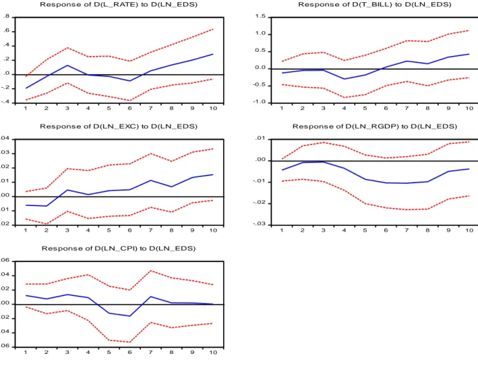
𝑌𝑡= [𝐸𝐷𝑆𝑡, 𝐿𝑅𝑡, 𝑇𝐵𝐼𝐿𝐿𝑡, 𝐸𝑋𝐶𝑡, 𝑅𝐺𝐷𝑃𝑡, 𝐶𝑃𝐼𝑡] (5) The results suggest a sharply negative effect on real output due to a shock on external debt service, which is in accordance with the analytical framework and a large set of literature supported by the argument that the repayment of external debt reduces resources available in the economy. Regarding the reaction of the exchange rate, the empirical evidence shows that the effect of external debt service tends to appreciate the domestic currency during 2 quarters and after that quarter domestic currency starts to depreciate. This suggests that the payment of the fixed debt obligation by the government will evaporate the external reserves leading to a depreciation of domestic currency. Further, the treasury bills rate responds negatively during 5 quarters to a shock in external debt service, but after 5 quarters starts to present a positive reaction. The similar response is giving the lending rate to an innovation on external debt service, but the result becomes significant after 6 quarters with a positive reaction. The behaviour displayed by the interest rate variables suggests an insignificant impact on external debt service in the short-run, but the opposite happens in the long-run, with a tendency to increase in both interest rate. Finally, the evidence shows that the price level reacts positively to a shock on external debt service, with the only negative reaction between 4 and 6 quarters.
This evidence supports the existence of an inflationary tendency through the external debt service.
Figure 3: Effects of positive shocks in EDS on L_RATE, T_BILL, EXC, RGDP, and CPI
4.4.2. Variance Decomposition
Table 3 provides the variance decomposition in percentage, where seeks to examine the macroeconomic effects of variation of RGDP, CPI, EXC, L_RATE and T_BILL rate to a shock or innovation in all endogenous variables, with special attention to the external debt service. The findings of the variance decomposition corroborate with impulse response
-.4 -.2 .0 .2 .4 .6 .8 1 2 3 4 5 6 7 8 9 10
Res pons e of D(L_RATE) to D(LN_EDS)
-1.0 -0.5 0.0 0.5 1.0 1.5 1 2 3 4 5 6 7 8 9 10
Res pons e of D(T_BILL) to D(LN_EDS)
-.02 -.01 .00 .01 .02 .03 .04 1 2 3 4 5 6 7 8 9 10
Res pons e of D(LN_EXC) to D(LN_EDS)
-.03 -.02 -.01 .00 .01 1 2 3 4 5 6 7 8 9 10
Res pons e of D(LN_RGDP) to D(LN_EDS)
-.06 -.04 -.02 .00 .02 .04 .06 1 2 3 4 5 6 7 8 9 10
Res pons e of D(LN_CPI) to D(LN_EDS)
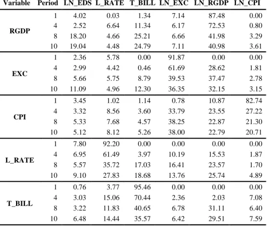
inference, where the external debt service accounts for a significant variation in real output (19.04%) and in the exchange rate (11.09%). Lastly, the variance decomposition analysis does not show a significant contribution of external debt service on the variation of general price level and on the interest rate variables. According to this analysis, the variation in the price level (38.25%) is significantly explained by changes in the exchange rate, which indicates the vulnerability of this economy to fluctuations in the exchange rate.
Table 3: Variance Decomposition (%)
Variable Period LN_EDS L_RATE T_BILL LN_EXC LN_RGDP LN_CPI
RGDP 1 4.02 0.03 1.34 7.14 87.48 0.00 4 2.52 6.64 11.34 6.17 72.53 0.80 8 18.20 4.66 25.21 6.66 41.98 3.29 10 19.04 4.48 24.79 7.11 40.98 3.61 EXC 1 2.36 5.78 0.00 91.87 0.00 0.00 4 2.99 4.42 0.46 61.69 28.62 1.81 8 5.66 5.75 8.79 39.53 37.47 2.78 10 11.09 4.96 12.30 36.35 32.15 3.15 CPI 1 3.45 1.02 1.14 0.78 10.87 82.74 4 3.32 8.56 3.60 33.79 23.55 27.22 8 5.33 7.68 4.57 38.25 22.87 21.30 10 5.12 8.12 5.26 38.00 22.79 20.71 L_RATE 1 7.80 92.20 0.00 0.00 0.00 0.00 4 6.95 61.49 3.97 10.19 15.53 1.87 8 5.57 35.72 17.03 16.41 23.57 1.70 10 9.10 27.83 18.68 13.76 25.74 4.89 T_BILL 1 0.76 3.77 95.46 0.00 0.00 0.00 4 3.03 15.06 70.44 2.36 2.03 7.08 8 3.22 11.83 40.65 6.78 31.11 6.40 10 6.48 14.44 35.57 6.42 29.51 7.59
4.5. Model 4
4.5.1. Impulse response
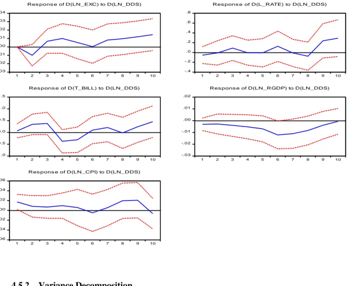
The impulse response function of an unexpected positive shock in the domestic debt service is shown in Figure 4, after estimating the following model:
𝑌𝑡= [𝐸𝑋𝐶𝑡, 𝐷𝐷𝑆𝑡, 𝐿𝑅𝑡, 𝑇_𝐵𝐼𝐿𝐿𝑡, 𝑅𝐺𝐷𝑃𝑡, 𝐶𝑃𝐼𝑡] (6) The results demonstrate that real output responds negatively to a shock on domestic debt service, and this effect is felt during all periods. It supports the idea that the payment of the fixed debt obligation implies an outflow of domestic resources, and consequently contributes to a strong fall in real output. Regarding the interest rate variables, the results show that the treasury bills rate responds positively to innovation on domestic debt, but this effect is lived during 3 quarters, where it displays a negative reaction between 3 to 5 quarters. From 6 quarters onwards, the treasury bills rate shows again the positive reaction. The prevalence of a positive reaction on treasury bills rate on a positive shock of domestic debt service may suggest the continue issuing of domestic debt by the government even for repay the debt and to finance their expenditure. Lending rate shows a slightly positive reaction, but after 8 quarters there is a remarkable positive response. Overall, the evidence shows that in the long-run interest rate variables present a positive reaction. In addition, the results also show that exchange rate reacts negatively to a shock on domestic debt service, but this effect is short-lived. After 2 quarters it responds positively, which means a depreciation in domestic currency. Finally, the price level displays a positive reaction to an innovation on domestic debt service. Therefore, the behaviour of the general price level suggests the existence of an inflationary tendency given a positive shock on domestic debt service.
Figure 4: Effects of positive shocks in DDS on EXC, L_RATE, T_BILL, RGDP, and CPI
4.5.2. Variance Decomposition
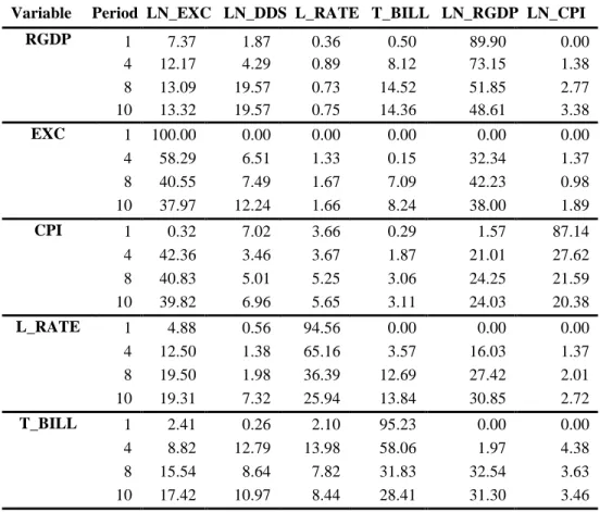
Table 4 presents the variance decomposition of real output, exchange rate, price level, lending rate and treasury bills rate to an innovation in all variables of model 5, mainly on domestic debt service. The results suggest that a shock in domestic debt service explains a significant variation in real output (19.57%), exchange rate (12.24%) and treasury bills rate (10.97%). Contrary to the findings from the impulse response analysis, domestic debt service does not account for significant variations in the general price level (less than 8%). However, -.03 -.02 -.01 .00 .01 .02 .03 .04 1 2 3 4 5 6 7 8 9 10
Res pons e of D(LN_EXC) to D(LN_DDS)
-.4 -.2 .0 .2 .4 .6 .8 1 2 3 4 5 6 7 8 9 10
Res pons e of D(L_RATE) to D(LN_DDS)
-1.0 -0.5 0.0 0.5 1.0 1.5 1 2 3 4 5 6 7 8 9 10
Res pons e of D(T_BILL) to D(LN_DDS)
-.03 -.02 -.01 .00 .01 .02 1 2 3 4 5 6 7 8 9 10 Res pons e of D(LN_RGDP) to D(LN_DDS) -.06 -.04 -.02 .00 .02 .04 .06 1 2 3 4 5 6 7 8 9 10
Res pons e of D(LN_CPI) to D(LN_DDS)
the variation in the price level is explained significantly by a shock in the exchange rate (42.36%) and by real output (24.25%).
Table 4: Variance decomposition (%)
Variable Period LN_EXC LN_DDS L_RATE T_BILL LN_RGDP LN_CPI RGDP 1 7.37 1.87 0.36 0.50 89.90 0.00 4 12.17 4.29 0.89 8.12 73.15 1.38 8 13.09 19.57 0.73 14.52 51.85 2.77 10 13.32 19.57 0.75 14.36 48.61 3.38 EXC 1 100.00 0.00 0.00 0.00 0.00 0.00 4 58.29 6.51 1.33 0.15 32.34 1.37 8 40.55 7.49 1.67 7.09 42.23 0.98 10 37.97 12.24 1.66 8.24 38.00 1.89 CPI 1 0.32 7.02 3.66 0.29 1.57 87.14 4 42.36 3.46 3.67 1.87 21.01 27.62 8 40.83 5.01 5.25 3.06 24.25 21.59 10 39.82 6.96 5.65 3.11 24.03 20.38 L_RATE 1 4.88 0.56 94.56 0.00 0.00 0.00 4 12.50 1.38 65.16 3.57 16.03 1.37 8 19.50 1.98 36.39 12.69 27.42 2.01 10 19.31 7.32 25.94 13.84 30.85 2.72 T_BILL 1 2.41 0.26 2.10 95.23 0.00 0.00 4 8.82 12.79 13.98 58.06 1.97 4.38 8 15.54 8.64 7.82 31.83 32.54 3.63 10 17.42 10.97 8.44 28.41 31.30 3.46 4.6. Model 5 4.6.1. Impulse response
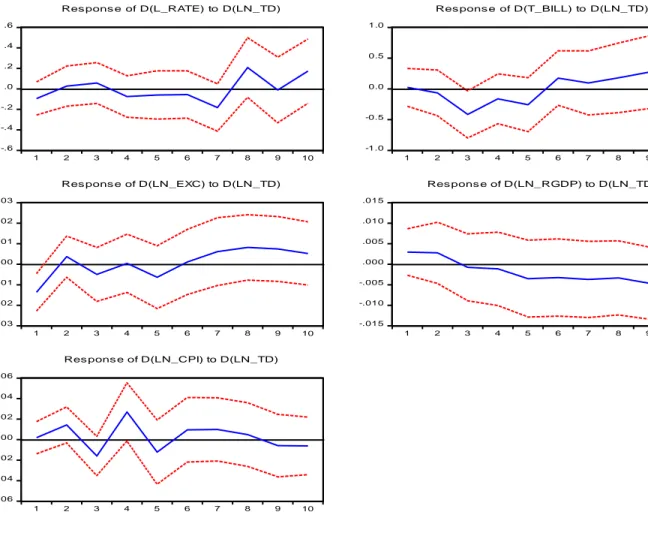
Figure 5 shows the results of the impulse response function of a shock in total debt, after estimating the following model:
The results suggest that total debt affects real output positively, but this effect is short-lived, and after 2 quarters it responds negatively. It means that the total public borrowing only gives positive effects in the economy in the short-run, but not in the long-run. The EXC respond negatively, but from quarter 6 starts to react positively, which means an appreciation in the domestic currency. The interest rate variables react negatively to an innovation in TD, but after quarter 6they start to respond positively for T_BILL and quarter 7th for L_RATE.
It means a long run effect of TD in these variables. The CPI shows many moments with the inflationary tendency which means a positive reaction.
Figure 5: Effects of positive shocks in TD on L_RATE, T_BILL, EXC, RGDP, and CPI
-.6 -.4 -.2 .0 .2 .4 .6 1 2 3 4 5 6 7 8 9 10
Res pons e of D(L_RATE) to D(LN_TD)
-1.0 -0.5 0.0 0.5 1.0 1 2 3 4 5 6 7 8 9 10
Res pons e of D(T_BILL) to D(LN_TD)
-.03 -.02 -.01 .00 .01 .02 .03 1 2 3 4 5 6 7 8 9 10
Res pons e of D(LN_EXC) to D(LN_TD)
-.015 -.010 -.005 .000 .005 .010 .015 1 2 3 4 5 6 7 8 9 10 Res pons e of D(LN_RGDP) to D(LN_TD) -.06 -.04 -.02 .00 .02 .04 .06 1 2 3 4 5 6 7 8 9 10
Res pons e of D(LN_CPI) to D(LN_TD)
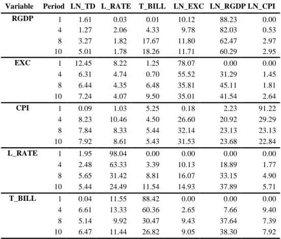
4.6.2. Variance Decomposition
Table 5 provides the results of the variance decomposition in percentage of real output, exchange rate, price level, lending rate and treasury bills rate to an innovation in all variables of model 5, mainly on total debt. It shows that the total debt shock only accounts significantly for variation of the exchange rate (12.45% in 1 quarter) and a small share of the variation (less than 9%) for the remaining variables of the model. In addition, the results suggest an important contribution of the exchange rate in the variation of most of the selected macroeconomic variables, an exception on treasury bills rate (less than 10%).
Table 5: Variance Decomposition (%)
Variable Period LN_TD L_RATE T_BILL LN_EXC LN_RGDP LN_CPI RGDP 1 1.61 0.03 0.01 10.12 88.23 0.00 4 1.27 2.06 4.33 9.78 82.03 0.53 8 3.27 1.82 17.67 11.80 62.47 2.97 10 5.01 1.78 18.26 11.71 60.29 2.95 EXC 1 12.45 8.22 1.25 78.07 0.00 0.00 4 6.31 4.74 0.70 55.52 31.29 1.45 8 6.44 4.35 6.48 35.81 45.11 1.81 10 7.24 4.07 9.50 35.01 41.54 2.64 CPI 1 0.09 1.03 5.25 0.18 2.23 91.22 4 8.23 10.46 4.50 26.60 20.92 29.29 8 7.84 8.33 5.44 32.14 23.13 23.13 10 7.92 8.61 5.43 31.53 23.68 22.84 L_RATE 1 1.95 98.04 0.00 0.00 0.00 0.00 4 2.48 63.33 3.39 10.13 18.89 1.77 8 5.65 31.42 8.81 16.07 33.15 4.90 10 5.44 24.49 11.54 14.93 37.89 5.71 T_BILL 1 0.04 11.55 88.42 0.00 0.00 0.00 4 6.61 13.33 60.36 2.65 7.66 9.40 8 5.14 9.92 30.47 9.43 37.64 7.39 10 6.47 11.44 26.82 9.05 38.30 7.92
4.7. Model 6
4.7.1. Impulse response
Figure 6 plots the repercussions of one standard deviation positive shocks in total debt service, after estimation the following model:
𝑌𝑡= [𝑇𝐷𝑆𝑡, 𝐿𝑅𝑡, 𝑇_𝐵𝐼𝐿𝐿𝑡, 𝐸𝑋𝐶𝑡, 𝑅𝐺𝐷𝑃𝑡, 𝐶𝑃𝐼𝑡] (8) The effect on real output is negative during all periods. This result is in accordance with the model framework and a set of studies, where the payment of debt service represents an outflow of resources reducing the availability of resources in the economy. The exchange rate reacts negatively to a shock in total debt service, but this effect is felt only during 2 quarters. After that, the exchange rate displays a positive response meaning a depreciation of domestic currency against the US dollar currency. The payment of external debt will contribute to reducing the country’s reserves in foreign currency leading to an appreciation of the external currency. Regarding the interest rate variables, the response on the treasury bills rate just becomes significant after 6 quarters, with a positive reaction to a shock in total debt service. The behaviour of the treasury bills rate suggests the possibility of continuous issuing of domestic debt by the government to relieve the debt service burden. The lending rate has a slightly positive response to an innovation in total debt service, but after 7 quarters this reaction sharply increases. Overall, in the long-run, the impulse response function suggests an increase in both interest rate variables due to a positive shock in total debt service. Lastly, the results suggest that after a total debt service shock, the general price level responds positively with a negative reaction from the 5 to 7 quarters, and then still shows a positive
reaction. This behaviour shows an inflationary tendency because of a positive shock in total debt service.
Figure 6: Effects of positive shocks in TDS on EXC, T_BILL, L_RATE, RGDP, and CPI
4.7.2. Variance Decomposition
Table 6 displays the results of the variance decomposition, in percentage, of selected macroeconomic variables to a shock in all variables of the model 6, with a special focus to a shock in total debt service. The results suggest that total debt service explains a significant percentage variation of real output (25.25%), exchange rate (17.67%) and the price level
-.4 -.2 .0 .2 .4 .6 .8 1 2 3 4 5 6 7 8 9 10
Res pons e of D(L_RATE) to D(LN_TDS)
-0.8 -0.4 0.0 0.4 0.8 1.2 1 2 3 4 5 6 7 8 9 10
Res pons e of D(T_BILL) to D(LN_TDS)
-.04 -.02 .00 .02 .04 .06 1 2 3 4 5 6 7 8 9 10
Res pons e of D(LN_EXC) to D(LN_TDS)
-.03 -.02 -.01 .00 .01 .02 1 2 3 4 5 6 7 8 9 10 Res pons e of D(LN_RGDP) to D(LN_TDS) -.04 .00 .04 .08 1 2 3 4 5 6 7 8 9 10
Res pons e of D(LN_CPI) to D(LN_TDS)
(9.85%). For the other endogenous variables, treasury bills rate and lending rate, total debt service shock accounts for a small variation (less than 7%). In addition, the results also show the important role played by the exchange rate (32.44%) and real output (24.11%) on variation in general price level. This evidence suggests the significant contribution of the exchange rate on a variation of the most variables of the model, mainly on the price level.
Table 6: Variance Decomposition (%)
Variable Period LN_TDS L_RATE T_BILL LN_EXC LN_RGDP LN_CPI
RGDP 1 2.48 0.00 1.24 4.30 91.96 0.00 4 4.66 2.96 11.33 8.14 72.13 0.78 8 24.99 2.60 18.38 8.82 42.58 2.63 10 25.25 2.71 18.06 9.10 41.81 3.07 EXC 1 1.12 6.53 0.01 92.33 0.00 0.00 4 8.21 3.80 0.69 54.45 30.95 1.91 8 8.61 4.16 8.90 37.52 39.26 1.54 10 17.67 3.64 9.99 33.24 33.15 2.31 CPI 1 1.12 3.26 0.33 1.57 2.92 90.80 4 2.44 10.79 2.25 30.27 21.39 32.86 8 7.27 8.55 3.25 32.44 24.11 24.38 10 9.85 8.31 3.39 31.60 23.86 22.99 L_RATE 1 2.02 97.98 0.00 0.00 0.00 0.00 4 1.88 65.37 3.65 8.26 18.78 2.05 8 1.55 37.64 15.22 16.52 26.57 2.50 10 6.22 28.53 17.56 15.10 28.57 4.03 T_BILL 1 0.28 2.62 97.09 0.00 0.00 0.00 4 3.68 15.30 68.93 3.51 1.65 6.92 8 2.84 11.09 40.66 8.85 30.71 5.85 10 5.90 13.89 35.89 9.00 29.24 6.08
5. Conclusions
This dissertation has studied the effect of public debt and debt service on real output, general price level, exchange rate, treasury bills rate and lending rate with an empirical analysis of Mozambique, using quarterly time-series ranging from 2000Q1 to 2016Q4. Were developed six Vector Autoregression (VAR) model to assess separately the economic effect of public debt variables, namely: external, domestic and total debt and the debt service variable as the following: external, domestic and total debt service variable. The main results of the models were produced through the structural analysis of the VAR model, namely: impulse response functions and variance decomposition.
From the econometric analysis, the dissertation found that public external debt and total debt only had a positive effect on real output during few quarters but not in the long-run. In case of domestic debt, the real output responds negatively to innovation from this kind of debt, which follows our prediction from the analytical framework and some literature that the domestic debt will reduce the available resources in the economy. Regarding the debt service variables, for external, domestic and total debt service, the evidence shows strong decreases in real output. This result is in accordance with the analytical framework and many kinds of literature supported by the argument that the repayment of debt reduces the resources available in the economy. Overall, debt service had a deeply negative effect on real output and debt variables do not contribute to increase real output.
The study also found an ambiguous result in price level given shocks in external debt and total debt, which means that we cannot conclude anything about the inflationary tendency because of the ED. In addition, the model found a significant contribution of EXC and
L_RATE on the variation of the general price level, which can support the inflationary tendency through this channel. This behaviour was predicted by the framework, through the economic structure of Mozambique. This result shows the vulnerability of this economy in exchange rate fluctuation. The domestic debt had a positive effect in the price level in the short-run and recovery in the long-run. Despite the contribution of domestic debt in an increase in the price level, the model shows the significant contribution of EXC and RGDP on inflationary tendency. Debt service variables as external, domestic and total debt service had a positive effect on the price level, which suggests the existence of an inflationary tendency given an innovation in EDS. Overall, the variation in the price level accounted significantly for changes in EXC, which suggests that the price level is explained by EXC. In addition, the investigation shows an appreciation of domestic currency in the short-run and a depreciation of the domestic currency in the long-short-run given the increase in debt variables, namely: external, domestic and total debt. The use of sterilization mechanism by the Central Bank through the ED could explain the stabilization in EXC in the short-run. The domestic debt will affect EXC in the long-run. The debt service variables, namely: external, domestic and total lead to a depreciation in domestic currency against the US dollar currency. The payment of external debt obligation will contribute to reducing the country’s reserves in foreign currency leading to an appreciation of the external currency. It means that EDS exposes the country to exchange rate fluctuation risk. Overall, the debt service variables accounted significantly for variation in EXC when compared to debt variables.
External debt, in the short-run, does not account significantly for the variation of interest rate variables because the government will be using the external resource, realizing the domestic resource. Similarly, the interest rate variables did not respond to innovation in
domestic debt, but in the long-run account for a significant contribution to the variation in the T_BILL rate in quarter 10th with 10.86% and not for other variables. It means that the
successive issuing of DD will increase the T_BILL rate and consequently affect positively the L_RATE.
The behaviour of interest rate variables suggests the insignificant impact of EDS in the short-run, but in the long-run, there is a tendency to increase in both interest rate, mainly in the lending rate. The DDS had a positive reaction in the interest rates with a significant reaction in the long-run, which implies an increase in interest rate given an innovation in DDS.