Fiscal Sustainability: A Panel Assessment for Advanced Economies

(1)

António Afonso & João Tovar Jalles

Fiscal Sustainability: A Panel Assessment for

Advanced Economies

WP05/2015/DE/UECE _________________________________________________________ De pa rtme nt o f Ec o no mic s

WORKING PAPERS

(2)

F

ISCAL

S

USTAINABILITY

:

A

P

ANEL

A

SSESSMENT FOR

A

DVANCED

E

CONOMIES

*

António Afonso

$

, João Tovar Jalles



Abstract

We assess the sustainability of public finances in OECD countries using panel unit root and cointegration analyses. Results show: no cointegration (no sustainability) between revenues and expenditures; improvement of the primary balances after worsening debt ratios; causality from government debt to primary balances.

JEL: C33, E62, H62, H63

Keywords: debt, primary balance, stationarity, panel analysis, FMOLS

_____________________________

*_{We are grateful for comments at ECB, and ISEG seminars, and at the INFER Annual Conference. The opinions expressed}

herein are those of the authors and not necessarily those of their employers.

$_ISEG/ULisbon_–_{University of Lisbon, Department of Economics; UECE}_–_{Research Unit on Complexity and Economics, R.}

Miguel Lupi 20, 1249-078 Lisbon, Portugal, email: [email protected]. UECE is supported by the Portuguese Foundation for Science and Technology through PEst-OE/EGE/UI0436/2011.

(3)

1. Introduction

The importance of sustainable public finances has received increasing attention following the 2008-2009 financial crisis. Sustainable fiscal policies can be continued, theoretically without changes in the policy stance, while the intertemporal government budget constraint holds. Conversely, if budgetary imbalances prevail, changes would be required, implying larger economic adjustments.

We investigate the sustainability of fiscal policy in a panel of 18 OECD countries in the period 1970-2010. We use stationarity analysis of the first-differenced stock of government debt and assess cointegrating between government revenues and expenditures, and between primary balances and debt, derived from the intertemporal government budget constraint. These approaches provide an indirect test on the solvency of public finances.

Our results suggest that long-run causality runs from lagged debt to primary balance, but on average the marginal long-run impact is zero. We cannot say that fiscal policy has been sustainable for most countries in our sample.

2. Theoretical Framework

A sustainable fiscal policy should ensure that the present value of the stock of public debt goes to zero in infinity, constraining the debt to grow no faster than the real interest rate (no Ponzi game). Recalling the Present Value Budget Constraint, it is possible to present analytically two definitions of sustainability suitable for empirical testing (Hamilton and Flavin, 1986):

i) The value of current public debt equals the sum of future primary surpluses; ii) The present value of public debt approaches zero in infinity.

To test the absence of Ponzi games, we inspect the stationarity of the first difference of the stock of debt, B_t, and cointegration between primary balance, s, and the (lagged) stock of the public debt, Bt (Bohn, 2007):

t t

t B u

s  _₁ (1)

This “backward-looking” approach implies that past increases in the level of debt would imply larger primary balances today. Such relationship has been mentioned in the context of the Fiscal Theory of the Price Level and the distinction between Ricardian and non-Ricardian fiscal regimes.

(4)

also stationarity. With the no-Ponzi game condition, GG_t and R_t must be co-integrated variables of order one for their first differences to be stationary. The procedure involves testing the following cointegrating regression:

t t

t GG u

R   (2)

and if the null of no co-integration is rejected, u_t must be stationary.

3. Methodology and Results

There has been a fair amount of empirical studies on fiscal sustainability notably for the US and Europe (Feve and Henin, 2000; Afonso, 2005; Camarero et al., 2014). However, given the low power of individual country-by-country tests, it may be preferable to pool the time series and conduct panel analysis, also justified by the economic and financial integration of the economies and their interdependences.

We implement two panel unit root tests: first generation tests, the Im et al. (2003) test (IPS) and second generation tests – Cross-Sectionally Augmented Panel Unit Root Test (CIPS test). The latter tests account for cross-sectional dependence of the contemporaneous error terms (Pesaran, 2007).

The outcome for the full sample is as follows: the null hypothesis of unit roots for the panel for debt, total government expenditures, revenues and the primary balance cannot be rejected with the variables in levels (results available upon request).

Therefore, we implement the panel cointegration tests proposed by Pedroni (2004), residual-based tests for the null of no cointegration in heterogeneous panels. Two classes of statistics are considered. The first is based on pooling the residuals of the regression along the within-dimension of the panel; the second is based on pooling the residuals of the regression along the between-dimension of the panel.

Table 1 shows the outcomes of the cointegration between total government revenues and expenditures and the primary balance and (lagged) debt.1 We use four within-group tests and three between-group tests to check panel cointegration. The columns labelled within-dimension contain the computed value of the statistics based on estimators that pool the autoregressive coefficient across different countries for the unit root tests on the estimated residuals. The columns labelled between-dimension report the computed value of the statistics based on estimators that average individually calculated coefficients for each country. Both results show _____________________________

1

(5)

that the null hypothesis of no cointegration can be rejected. Therefore, the relationships identified in (1) and (2) are cointegrated for the panel of the country sample.

[Table 1]

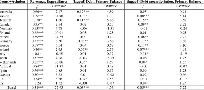
Assuming that government revenues and expenditures (government debt and primary balance) are cointegrated, we estimate the cointegrating coefficients to investigate the long-run relationship. We apply the between-dimension panel fully modified OLS (FMOLS) (Pedroni, 2000).2 Individual estimates and standard errors for H₀:i 0 in (1) and (2) are reported also for the panel.

For the pool of all countries taken together we get 0.51 and 0.03 (statistically significant at the 1% level) for the revenues-expenditures and primary balance-debt relationships, respectively (Table 2). In general, the results point to a positive long-run co-movement between the levels of government revenues and expenditures. On the second relationship, the average result points to solvency, although, a country-by-country inspection shows that only Australia, Belgium, Germany, Ireland, Netherlands and the UK present significant positive coefficient estimates for the improvement of the primary balance after past debt increases.

[Table 2]

If in each country Rtand GGt are individually non-stationary but together are cointegrated,

we know from the Granger representation theorem that these series can be represented in the form of a dynamic error correction model:

it K j j it ij K j j it ij it i it it it K j j it ij K j j it ij it i it it R GG e c GG GG R e c R 2 1 22 1 21 1 2 1 1 12 1 11 1 1 ˆ ˆ                        



         

. (3)

it i t i it

it R b GG

eˆ  ˆ  ˆ ˆ is the disequilibrium term and represents how far our variables are from the equilibrium relationship and the error correction mechanism estimates how this disequilibrium causes the variables to adjust towards equilibrium. Moreover, at least one of the adjustment coefficients 1i or 2imust be non-zero if a long-run relationship between the

variables holds. A test for the significance of 1i(2i) for any country can be interpreted as

_____________________________

2

(6)

whether shocks in government expenditures (revenues) have a long-run effect on government revenues (expenditures) and testing the sign of the ratio ₁_i/₂_ican be interpreted as a test of the sign of the long-run effect of shocks to government expenditures on revenues.

In practice, we use both group mean based tests and lambda-Pearson based tests. The combination of the two can be particularly informative when the underlying parameters of interest are heterogeneous. For instance, when

1 

t fails to reject he null while 1 

P succeeds in rejecting the null, this can be interpreted as a situation in which we do not reject that the average value for 1iis zero, even though we reject that it is pervasively zero in the panel.

[Table 3]

In Table 3 panel A, the ₁_iparameters reported indicate that long-run causality that does not run from expenditures to revenues (p-values above 10%). This supports the non-validity of the

“Spend and Tax” hypothesis, meaning that fiscal authorities are not able to generate the revenues required to finance planned expenditures. Turning to2i, we reject the hypothesis that

revenues have a zero average long-run effect globally (group mean tests) on spending. The results hold pervasively among individual countries and on average for the entire panel (based on the group-mean and Lamba-Pearson tests). The implication of these results is that changes in revenues induce permanent changes in long-run expenditures, the average marginal long-run impact being zero.

In Table 3 panel B, from the ₁_iparameters we conclude that long-run causality runs from lagged debt to the primary balance (p-values below 10%). The results hold among individual countries and on average for the entire panel. Turning to2i, we cannot reject the hypothesis

that primary balances have a zero average long-run effect globally (group mean tests). At the same time, the sign of the effect is mixed, so that the average is still zero. Again, the average marginal long-run impact is zero.

4. Conclusion

(7)

balances, the average marginal long-run impact is zero. Overall, fiscal policy has been unsustainable.

References

Afonso, A. (2005), “Fiscal Sustainability: the Unpleasant European Case”, FinanzArchiv, 61, 19-44.

Bohn, H. (2007), “Are Stationarity and Cointegration Restrictions Really Necessary for the Intertemporal

Budget Constraint?” Journal of Monetary Economics, 54, 1837-1847.

Camarero, M., Carrion-i-Silvestre, J., Tamarit, C. (2014), “The relationship between debt level and fiscal

sustainability in Organisation for Economic Cooperation and Development Countries”, Economic

Inquiry, online first.

Feve, P., Henin, P.Y. (2000), “Assessing Effective Sustainability of Fiscal Policy within the G-7”, Oxford Bulletin of Economics and Statistics, 62, 175.

Hamilton, J., Flavin, M.A. (1986), “On the Limitations of Government Borrowing: A Framework for

Empirical Testing”, American Economic Review 76, 808-819.

Im, K.., Pesaran, M., Shin, Y. (2003), “Testing for unit roots in heterogeneous panels”, Journal of Econometrics, 115, 53-74.

Pedroni P. (2004), “Panel Cointegration; Asymptotic and Finite Sample Properties of Pooled Time series

Tests, with an Application to the PPP Hypothesis,” Econometric Theory, 20, 597-625.

Pedroni, P. (2000), “Fully Modified OLS for Heterogeneous Cointegrated Panels”, in Baltagi, B., C.

Kao, Eds., Advances in Econometrics, Nonstationary Panels, Panel Cointegration and Dynamic

Panels, Elsevier Science, NY, 93-130.

Pesaran, M., (2007), “A simple panel unit root test in the presence of cross section dependence”, Journal

(8)

Table 1: Panel cointegration tests

relation Revenues and

Expenditures

(lagged) Debt and Primary Balance

(lagged) Debt-mean deviation and Primary Balance

No trend Trend No trend Trend No trend Trend

Within-dimension

Panel v 3.42 1.15 5.29 2.85 5.12 2.85

Panel  -2.93* -1.82* -3.98* -3.48* -3.78* -3.4*

Panel PP -2.61* -2.87* -3.07* -3.83* -2.92* -3.74*

Panel ADF -2.51* -2.75* -1.72 -1.91 -1.72 -1.92

Between-dimension

Group  -1.80 -0.55 -2.91* -1.58 -2.89* -1.57

Group PP -2.50* -2.48* -2.86* -3.15* -2.81* -3.12*

Group ADF

-2.51* -3.17* -1.81 -1.80 -1.93 -1.83

The null hypothesis is that there is no cointegration. An asterisk (*) indicates rejection at the 10% level or better.

Table 2: Panel estimates of the cointegrating relationship (FMOLS)

Country\relation Revenues, Expenditures (lagged) Debt, Primary Balance (lagged) Debt-mean deviation, Primary Balance  t-statistic  t-statistic  t-statistic

Australia 0.60** 2.47 0.17*** 4.59 0.05 0.91

Austria 0.69*** 14.98 0.03* 1.98 0.08*** 5.14

Belgium 0.30* 1.80 0.11*** 5.16 0.15** 3.58

Canada 0.35** 2.34 0.02 0.55 0.09** 2.22

Denmark 0.63*** 4.78 -0.06 -1.51 -0.01 -0.24

Finland 0.68*** 10.01 0.05 1.25 0.01 0.95

France 0.69*** 14.25 0.00 0.12 0.06** 2.72

Germany 0.53*** 6.50 0.08** 3.66 0.11** 3.68

Greece 0.67*** 6.54 0.04 0.69 0.11** 3.10

Ireland 0.40** 2.65 0.07** 2.57 0.07*** 4.94

Italy -0.14 -0.45 0.01 0.37 -0.04* -2.19

Japan 0.52*** 4.28 -0.03 -3.15 0.06 1.45

Netherlands 0.65*** 16.06 0.05* 1.59 0.04* 1.63

Portugal 0.84** 11.87 0.01 0.48 -0.00 -0.07

Spain 0.76*** 9.85 0.01 0.17 0.09 1.23

Sweden 0.50*** 5.52 -0.01 -0.08 0.02 0.56

UK 0.34** 3.36 0.07* 1.83 -0.01 -0.17

US 0.24 1.52 -0.00 -0.07 0.04 1.23

Panel 0.51*** 27.93 0.03*** 4.76 0.05*** 7.22

The regressions estimated correspond to Eq. (1) and (2) in the main text. *, **, *** denote significance at 10, 5 and 1% levels.

Table 3: Panel Long-run Causality

Panel A: it it R GG  : 1

 2:RitGGit 1/2

Estimate Test p-value Estimate Test p-value median

Group mean 0.14 0.24 0.60 0.34 2.31 0.01 -0.55

Lamba-Pearson 47.35 0.10 145.39 0.00 0.42

Panel B:

it

it s

B_₁

1:

 2:sit Bit1 1/2

Estimate Test p-value Estimate Test p-value median

Group mean 0.66 1.56 0.06 -0.42 -1.18 0.12 0.97

Lamba-Pearson 104.58 0.00 90.64 0.00 0.41