GOVERNMENT INDEBTEDNESS AND EUROPEAN CONSUMERS BEHAVIOUR

GOVERNMENT INDEBTEDNESS AND EUROPEAN CONSUMERS

BEHAVIOUR

António Afonso(**)

Department of Economics, Instituto Superior de Economia e Gestão, Universidade Técnica de Lisboa,

R. Miguel Lúpi, 20, 1249-078 Lisbon, Portugal This version: October 2001

Abstract

According to conventional macroeconomics, public debt has a significant effect on the economy since consumers see public debt as net wealth, however, according to the Ricardian Equivalence hypothesis, that effect would be absent. This paper’s results, obtained from Euler equation estimations, using a panel data approach, indicate that it would be wise to reject the debt neutrality hypothesis for the EU-15. However, estimations carried out after dividing the countries into two groups, tentatively allow us to conclude that private consumption in "less indebted" countries seems to be more responsive to wealth increases than in the "more indebted" countries.

Keywords: Deficit finance; Ricardian equivalence; Private consumption; European Union; panel data

JEL classification: C23; E21; E62; H63

(*)

This paper was part of the research project for the author’s Ph.D. thesis. The author acknowledges comments on previous versions from Jorge Santos, João Santos Silva and from participants at seminar and conferences in Lisbon and Ankara. The usual disclaimer applies.

(**)

1. Introduction

Government debt neutrality and the Ricardian Equivalence hypothesis have been one of the most debated issues of modern macroeconomics, and the subject of a large number of theoretical and empirical research papers. Under conventional macroeconomic analysis, public debt has an effect on the economy since consumers consider public debt as net wealth.1 Therefore, the bigger the stock of public debt the wealthier consumers feel and the more inclined they are to consume.

The terms “Ricardian Equivalence Theorem” or “Ricardian Equivalence Proposition” are nowadays included in the vocabulary of macroeconomics being the expression Ricardian Equivalence apparently coined by Buchanan (1976).2 While the first formal exposition is credited to Barro (1974), in a seminal paper, the theoretical rational behind the Ricardian Equivalence hypothesis was originally stated by Ricardo (1817, 1820).3 Even if Barro does not initially refer Ricardo, he ends up acknowledging Ricardo’s merit in his reply to Buchanan’s (1976) comment.4

This paper adds to the existing literature, by using panel data methodology in testing the debt neutrality hypothesis, which so far was basically tested using time-series methods. As far as the author knows, this is also the first investigation, concerning debt neutrality, aiming exclusively at the EU countries.

The paper is organised as follows: in section two, Barro’s result for debt neutrality is briefly discussed; section three derives the Euler equation set up, resulting from the consumer’s inter-temporal optimisation problem; section four presents the empirical results for the EU-15, and offers some comments; section five is a conclusion.

1

See for instance Blinder and Solow (1973) and Christ (1978). 2

Feldstein (1982) prefers the term pre-Ricardian Equivalence hypothesis or proposition. Buiter and Tobin (1979) use the expression neo-Ricardian Equivalence.

3

Barro (1998, pp. 47) guesses that his 1974 article has probably been quoted more that 840 times. 4

2. Government debt neutrality

Barro’s (1974) paper definitely set a landmark and represented a turning point of the literature concerning the public debt issue. The necessary conditions for the Ricardian Equivalence to hold are clearly presented on that paper, namely the intergenerational solidarity model, with a theoretical set up inspired in the overlapping generations model of Samuelson (1958) and Diamond (1965).5 Definitely, the link between generations is paramount to guarantee the debt neutrality result.

In a simplified way, the main idea of the debt neutrality proposition dwells on the supposition that public debt and lump sum taxes are equivalent methods of financing a given amount of public expenses. Deficits merely postpone the future imposition of taxes. If consumers are rational, it becomes indifferent to pay 100 Euros of taxes today or tomorrow. In that sense, being irrelevant to the consumers the moment when taxes are paid, consumers do not change their consumption decisions after variations in the budget deficit. Therefore, one of the several implications of the theorem’s validity is the result of debt neutrality, when the deficit is financed by public debt, that is, deficits do not influence real variables, and have no effects on aggregate demand. For instance, Phelps (1982, pp. 379) considers that increases in the supply of public debt ends up creating its own demand, and it would not influence the demand for other assets. In other words, there would be a sort of “Say’s Law” for the deficits and its financing by public debt.

Nevertheless, one must recognize that Ricardo was convinced that in practice it was quite relevant the method the government chooses to finance its expenses. This conviction of Ricardo led O’Driscoll (1977) to suggest that the Ricardian Equivalence Theorem should be called “Ricardian Nonequivalence Theorem.”6

5

As Elmendorf and Mankiw (1999) put it, “Barro can be viewed as the Christopher Columbus of Ricardian Equivalence (…) Barro was not the first economist to discover Ricardian Equivalence, but he was surely the last (…) and no one will be able to discover it again.”

6

Usually, the critics to the Ricardian Equivalence hypothesis focus on distortionary taxation, and intergenerational altruism and capital markets efficiency.7 For instance, Sims (1998) states in a vigorous way that the Ricardian Equivalence theorem is irrelevant for the reality economists try to understand and formalise, while Buiter (1985) holds that “neutrality of public debt and deficits is little more than a theoretical curiosum.” It should therefore be considered as an extreme situation since taxes are not lump-sum, some prices are not perfectly flexible, people do not live forever and many people do not have ascendants or descendants willing to help them financially.

The altruistic behaviour is also open to much criticism and discussion. The absence of intergenerational transfers may for instance be the result of divergent preferences among household members.8 Also, the opposition between finite horizons and infinite horizons, for the validation of altruism, may not be that important when one considers budget deficits short run effects. Notice, for instance, that if public debt has an average maturity of 10 or 15 years, then there is a high probability that present generations will be called upon to finance debt redemption, through the imposition of future taxes, even if there is a certain amount of Ponzi games.

It is quite unlikely that capital markets are efficient or that households do not face liquidity constraints. One of the reasons for capital markets imperfections is the existence of credit rationing, eventually due to adverse selection or asymmetric information problems.9 Adverse selection in the capital markets, specifically in the credit market, is usually the main obstacle against the possibility of accepting Ricardian Equivalence. One may say that when a considerable part of consumers is liquidity constrained, favourable evidence for supporting Ricardian Equivalence should be quite

7

Discussions of the necessary conditions for Ricardian Equivalence to hold, may be found namely in Brennan and Buchanan (1986), Bernheim (1987, 1989), Aschauer (1988) and Seater (1993).

8

On this topic see Carmichael (1982) and Becker (1974). Laitner and Ohlsson (2001) present several versions of possible altruistic models.

9

feeble. As a matter of fact, in such a setting, many consumers will be led to eventually consume their entire income.10

3. Government debt neutrality and private consumption

According to conventional macroeconomic theory, deficits affect negatively private investment. In a closed economy, a deficit increase, financed in the market, would raise interest rates since the government is competing with the private sector for the available savings in the economy and that might also cause more inflation. Increasing interest rates would then have a negative stimulus on private investment.11 In an open economy, with capital mobility, the interest rate increase would appreciate the national currency and increase foreign demand by assets denominated in national currency. On the other hand, currency appreciation is bound to deteriorate the current account.

The key idea behind Ricardian Equivalence is that consumers are linked by intergenerational altruism, and also that they have a fairly good perception about the future taxes needed to repay the present increase in public debt. Consumer’s net wealth would be invariant between more debt today and more taxes tomorrow. By this reasoning, budget deficits would have no real effects and fiscal policy would be unable to change consumption, quite a different notion from the one sustained by Keynes. In a limit situation, as Gramlich (1989) noted, when the government reduces taxes, consumers just save more, for instance placing money in time deposit accounts, in order to help pay the higher future taxes, and consumption remains unchanged.

Empirical validation of the neutrality hypothesis, through the consumption function, may generically be divided into two categories: tests using reaction functions inspired in the Permanent Income/Life Cycle hypothesis and Euler equation tests resulting from the consumer’s inter-temporal optimisation problem, the approach used on this paper. The direct use of Euler equations derived from the intertemporal consumer’s maximisation

10

Cushing (1992) and Rockerbie (1997) present results for the US that seem to indicate that about 40 per cent of the consumers are liquidity constrained. Leiderman and Razin (1988) develop and test a model where part of the consumers also face liquidity constraints in the capital markets.

11

problem in this framework, follows the initial work of Hall (1978), and is adopted by Aschauer (1985), Dalamagas (1992) and Gupta (1992). By using the first order condition for the representative consumer it is possible to skip the problems surrounding the specification of consumer functions based on the Permanent Income/Life Cycle hypothesis.

Suppose the following expression for the aggregate consumption function, as the sum of non-human wealth and human wealth, broadly inspired in Blanchard (1985),

    

  

+ +

+

=

∑

=

+ − −

0

1 (1 )

) 1 (

i

i t t i t

t A E Y

C α ρ µ _{,0<α<1; (1)}

where Cis aggregate consumption in period; At-1 is the stock of assets at the end of t-1, that is, non-human wealth, including government debt held by the public; ρ is the real rate of return (assumed constant); Yt is the after tax labour income (human wealth); α is the marginal propensity to consume out of total wealth; Etis the expectation operator, conditional to the information known by consumers at period t and µ is the discount rate used by consumers to discount future labour income.

If µ = ρ, then consumers act as if they lived forever, that is, they take into consideration

the consumption decisions of future generations. In a nutshell, if µ = ρ, consumers are Ricardian. The bigger the µ, the bigger the myopia effect in present generations when considering future taxes, and if that were the case we would be in a situation of almost complete absence of Ricardian Equivalence.

With finite horizons, consumers may discount future income at a discount rate higher than the interest rate they receive from their holdings of non-human wealth. When

µ > ρ, consumers are expecting to receive the total actual value of interests on public

of future taxes. In other words, consumers are indeed assuming a discount rate for human wealth higher than the real interest rate.12

In order to reach a testable model from expression (1), this equation is going to be lagged one period, multiplied by (1+µ) and the result subtracted from (1). The final result is given by

[

]

t

t C A A Y u

C =(1+µ) ₋₁+α(1+ρ) ₋₁−(1+µ) ₋₂ −α(1+µ) ₋₁+ (2)

where

[

]

∑

= − +

−

₋

+

=

0

1

)

1

(

i

i t t t i

t

E

E

Y

u

α

µ

Assuming that available aggregate income may be either consumed or accumulated in assets,

1

1 −

−

=

+

−

+

t

A

C

A

A

Y

ρ

the economy’s budget constraint is then given by

t t t

t A Y C

A = (1+ ρ) ₋₁ + − . (5)

Using equation (2) and (5) to eliminate human wealth from (10), the aggregate consumption function may be written as13

t t t

t C A u

C =(1+µ)(1−α) ₋₁ +α(ρ−µ) ₋₁ + (6)

12

Notice that for instance Evans (1988, pp. 985-986), one of the first authors to use this approach, uses a slightly different notation from the one used in this paper. The term (1+µ) in this paper is equivalent to the term (1−µ)/(1+ρ) on Evans paper. In Evans notation µ is the fraction of population that dies each period and, when µ = 0, consumers are Ricardian, they have infinite horizons, and when µ > 0, consumers have finite horizons. Evans (1993) interprets this fraction (probability) as a measure of the intensity of the existing links between actual consumers and futures generations. 13

and the testable model is then

t t

t

t C A u

C = β + δ ₋₁ + θ ₋₁ + , (7)

where β is a constant, δ = (1+µ)(1−α), and θ = α(ρ−µ). With equation (7) it is then possible to test if consumers are Ricardian. Specifically, the null hypothesis of Ricardian Equivalence is θ = 0 (ρ=µ). Under the alternative hypothesis, when consumers do not have a Ricardian behaviour (µ ≠ ρ ) , then the coefficient θ might be significantly different from zero. As explained above, this might imply that consumers behave as having finite horizons and government bonds are seen as net wealth.

4. Empirical tests for the EU: results and comments

After the 1st of January 1999 several European currencies gave way to the Euro. Eleven countries (Austria, Belgium, Finland, France, Germany, Ireland, Italy, Luxembourg, Netherlands, Portugal and Spain) successfully met the convergence criteria underlined in the Maastricht Treaty and, according to the decisions of the European Council of May 1998, those countries were the founders of Economic and Monetary Union. Four other countries of the European Union remained outside the Euro either, because they wanted, United Kingdom and Denmark, or because they did not fulfil the convergence criteria, Greece and Sweden. At the beginning of 2001, Greece also joined the Euro.

respectively for developing countries and for a set of both developing and OECD countries.

In this paper, to estimate equation (7), data for private consumption and government debt is used, with this last variable being a proxy for wealth. This option was chosen since it was impossible to get data for the monetary aggregates for every UE country, from a single source, in order to guarantee data comparability.14 All variables are in real terms, in 1990 prices, and expressed in Euros (data sources are describe in the Annex).

The strategy followed in this paper starts with dividing the countries into two groups, according to the indebtedness level. The debt-to-GDP ratio is used to classify the countries either as a “less indebted” country, when the debt-to-GDP ratio is below 60 per cent, or as a “more indebted” country, when the debt-to-GDP ratio is above 60 per cent. This approach allows the construction of an artificial variable, D1, which is equal to 1 for the “less indebted” countries, and assumes the value 0 for the countries classified as “more indebted”, that is,

  

> ≤ =

0,6 ratio

if , 0

0,6 ratio

if , 1 1

D . (8)

The reason for choosing initially the 60 per cent threshold is simply because this became an important limit for the debt-to-GDP ratio after the Maastricht Treaty. However, this limit will be allowed to change in the subsequent empirical work.

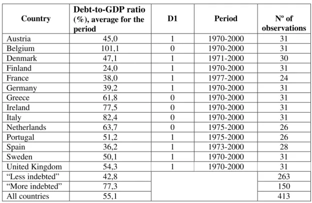
As a first working hypothesis, the debt-to-GDP ratio was computed for each country, as an average for the period 1970-2000. Those average ratios, the exact time span for each country and the binary values assigned to the artificial variable D1, are identified in Table 1 (Luxembourg was excluded due to data problems).

14

Table 1 – “Less indebted” and “more indebted” countries

Country

Debt-to-GDP ratio

(%), average for the period

D1 Period Nº of

observations

Austria 45,0 1 1970-2000 31

Belgium 101,1 0 1970-2000 31

Denmark 47,1 1 1971-2000 30

Finland 24,0 1 1970-2000 31

France 38,0 1 1977-2000 24

Germany 39,2 1 1970-2000 31

Greece 61,8 0 1970-2000 31

Ireland 77,5 0 1970-2000 31

Italy 82,4 0 1970-2000 31

Netherlands 63,7 0 1975-2000 26

Portugal 51,2 1 1975-2000 26

Spain 36,2 1 1973-2000 28

Sweden 50,1 1 1970-2000 31

United Kingdom 54,3 1 1970-2000 31

“Less indebted” 42,8 263

“More indebted” 77,3 150

All countries 55,1 413

The complete panel data sample includes 413 observations, divided into the two groups: “less indebted” countries, 263 observations and “more indebted” countries, 150 observations.

For the entire data sample, using panel data methodology, an equation inspired on equation (7) was estimated,

it i it

it

it

C

A

D

u

C

=

β

+

δ

+

θ

+

γ

1

+

Table 2 – Estimation of equation (9), pooled regression, dummy variable computed as the period average for each country

Variable (coefficient)

Linear model Logarithmic model

Constant (β) -3,851

(-2,109)

0,037 (2,640)

δ (Cit-1) 0,983

(118,089)

0,977 (150,371)

θ (Αit-1) 0,030

(3,630)

0,015 (2,683)

γ (D1) 5,757

(2,641)

0,025 (3,293)

_ 2

R _{0,9928 0,9968}

DW 0,959 0,925

The t statistics are in parenthesis. The DW statistics are computed according to Bhargava, Franzini e Narendanathan (1982), using TSP, version 4.4, 1997.

The estimation results do not discard the possibility of D1 being statistically different from zero. In other words, it is not possible to reject the idea that there are differences between consumers’ decisions in the “less indebted” and in the “more indebted” countries, after changes in wealth (here proxied only by government debt). Still another result to notice is that for the entire panel data sample, an increase in wealth has a positive effect on private consumption.

Subsequently, a different approach was tried, with the values for the artificial variable D1 being obtained on a year-by-year basis, for each country, according to the debt-to-GDP ratio observed in each year. This adjustment is important since several countries changed considerably their level of indebtedness during the period considered in this paper.

it it it

it i

it

C

A

D

u

C

=

β

+

δ

+

θ

+

γ

1

+

where βi stands for the individual effects to be estimated for each country i.

The fixed effects model is a typical choice for macroeconomists, and may eventually be more adequate than the random effects model. For instance, if the individual effects are somehow a substitute for non-specified variables, it is probable that each country specific effects are correlated with the other independent variables. In addition, and since the country sample includes all the relevant countries, the EU countries, it is less obvious that one might want to consider this set of countries as a random sample of a larger universe of countries.

In other words, and as reminded by Greene (1997) and Judson and Owen (1997), when the individual observations sample (countries in our case) comes from a larger population (which could be all the countries in the world), it would be suitable to consider the specific constant terms as randomly distributed through the cross section units. However, and even if the present country sample includes a small number of countries, it is sensible to admit that the EU-15 countries have similar specific characteristics, not shared by the other countries in the world. In this case, it would seem adequate to choose the fixed effects formalization, even if it is not correct to generalize the results afterwards, to the entire population, which is not the purpose of the paper.

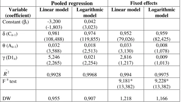
Table 3 – Estimation of equation (10), dummy variable computed for each year

Pooled regression Fixed effects

Variable (coefficient)

Linear model Logarithmic model

Linear model Logarithmic model Constant (βi) -3,200

(-1,803)

0,042 (3,023)

δ (Cit-1) 0,981

(108,488) 0,974 (119,855) 0,952 (79,026) 0,959 (82,425)

θ (Αit-1) 0,032

(3,588) 0,018 (2,513) 0,033 (3,130) 0,008 (1,078)

γ (D1it) 5,246

(2,265) 0,021 (2,254) 2,816 (1,217) 0,009 (1,013) _ 2

R 0,9928 0,9968 0,994 0,9975

F a test 9,181*

(13,382)

9,228* (13,382)

DW 0,955 0,907 1,218 1,166

The t statistics are in parentheses.

a - The degrees of freedman for the F statistic are in parentheses; the statistic tests the fixed effects model against the pooled regression model, where the autonomous term is the same for all countries, which is the null hypothesis.

* - Statistically significant at the 10 percent level, the null hypothesis, of the pooled regression model, is rejected

The possibility of the fixed effects model being more adequate seems to get statistical validation as one may confirm by the value of the F statistic. This is a test of the null hypothesis that all effects are the same for each country, in other words, the hypothesis that all autonomous terms βi for equation (10) are identical.15 However, with D1 entering equation (10) in an additive form, the statistical significance of this variable is rather low in the fixed effects model.

Still another alternative model was estimated, which includes the variable D1 in a multiplicative form in the private consumption equation, according to the following specification

15

The F statistic is computed as F (n-1, nT-n-k)=[(Ru 2

-Rp 2

)/(1- Ru 2

it it

it it

i

it C A D A u

C = β +δ ₋1 +θ ₋1 +ψ ( 1× ) ₋1 + , (11)

and the testable hypothesis implies to evaluate if ψ>0.

When public indebtedness is seen by the consumers as moderate (D1=1), changes in government debt would have a more significant effect on private consumption decisions, with that effect being given by [θ+ψ]. If government indebtedness is higher (D1=0), changes in public debt may have a more mitigated effect on private consumption, that is, consumers might become more Ricardian. Table 4 presents the estimation results for equation (11).

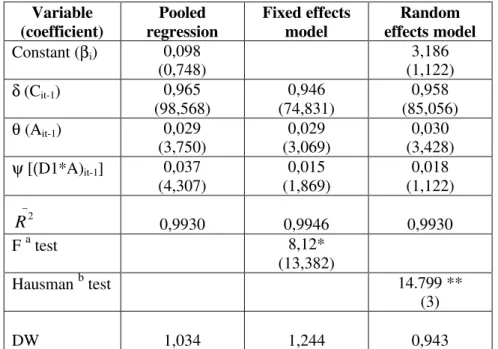
Table 4 – Estimation of equation (11), dummy variable computed for each year

(linear model) Variable (coefficient) Pooled regression Fixed effects model Random effects model Constant (βi) 0,098

(0,748)

3,186 (1,122)

δ (Cit-1) 0,965

(98,568)

0,946 (74,831)

0,958 (85,056)

θ (Αit-1) 0,029

(3,750)

0,029 (3,069)

0,030 (3,428)

ψ [(D1*A)it-1] 0,037

(4,307) 0,015 (1,869) 0,018 (1,122) _ 2

R 0,9930 0,9946 0,9930

F a test 8,12*

(13,382)

Hausman b test 14.799 **

(3)

DW 1,034 1,244 0,943

The t statistics are in parentheses.

a - The degrees of freedman for the F statistic are in parentheses; the statistic tests the fixed effects model against the pooled regression model, where the autonomous term is the same for all countries, which is the null hypothesis.

b - The statistic has a Chi-square distribution (the degrees of freedom are in parentheses); the Hausman (1978) statistic tests the fixed effects model against the random effects, which is here the null hypothesis.

* - Statistically significant at the 10 percent level, the null hypothesis of the pooled regression model is rejected.

Some comments can be made to those results. For instance, an increase of government debt of say 1000 Euros may have the effect of raising private consumption by 44 Euros (44=29+15, according to the fixed effects model), if government indebtedness is not too high (D1=1). This effect may amount to only 29 Euros when consumers, due to a more significant debt-to-GDP ratio (D1=0), assume a partially Ricardian behaviour. In this case, consumers perceive the increase of government debt, less as an increase of wealth and more as a sign of future tax increases.

Table 4 reports also the results for the random effects model. The feasibility of the random effects model is assessed by the Hausman statistic, which tests the null hypothesis that the random effects are not correlated with the explanatory variables. In our case, and taking into account the fact that the test statistic is significant at the 1 per cent level, the random effects model hypothesis is rejected, in favour of the fixed effects model.

Table 5 – Estimation of equation (10), two groups of countries

“Less indebted” countries

Variable (coefficient) Pooled regression Fixed effects model Random effects model Constant (βi) -0,437

(-0,233)

4,441 (1,155)

δ (Cit-1) 0,958

(83,661)

0,945 (63,688)

0,957 (72,583)

θ (Αit-1) 0,077

(5,586) 0,044 (3,199) 0,050 (3,690) _ 2

R 0,9925 0,9938 0,9924

F a test 7,60*

(8,243)

Hausman b test 10.978 **

(2)

DW 1,004 1,219 0,925

“More indebted” countries

Variable (coefficient) Pooled regression Fixed effects model Random effects model Constant (βi) 1,186

(0,881)

1,484 (1,823)

δ (Cit-1) 0,974

(77,097)

0,937 (35,151)

0,976 (73,304)

θ (Αit-1) 0,013

(1,481) 0,003 (-0,271) 0,010 (1,186) _ 2

R 0,9952 0,9953 0,9952

F a test 2,119*

(4,138)

Hausman b test 4.645 **

(2)

DW 1,217 1,217 0,943

The t statistics are in parentheses.

a - The degrees of freedman for the F statistic are in parentheses; the statistic tests the fixed effects model against the pooled regression model, where the autonomous term is the same for all countries, which is the null hypothesis.

b - The statistic has a Chi-square distribution (the degrees of freedom are in parentheses); the Hausman (1978) statistic tests the fixed effects model against the random effects, which is here the null hypothesis.

* - Statistically significant at the 10 percent level, the null hypothesis of the pooled regression model is rejected.

It is now possible to see that government debt seems more important to explain private consumption decisions in the “less indebted” countries, than in the “more indebted” countries. In fact, in the “less indebted” countries the government debt coefficient is positive and statistically different form zero, while for the group of “more indebted” countries, it is not possible to reject the hypothesis of that coefficient being different from zero in the private consumption function.

Therefore, in the case of the “less indebted” countries, and using the fixed effects model results, an increase of government debt of for instance 1000 Euros may have the effect of raising private consumption by 44 Euros, a result similar to the one previously found when estimating equation (11) for the entire country sample. One may then tentatively say that these results indicate somehow that private consumption in “less indebted” countries reacts more to government debt increases than consumption in “more indebted” countries.16 In other words, consumers would be less Ricardian in “less indebted” countries.

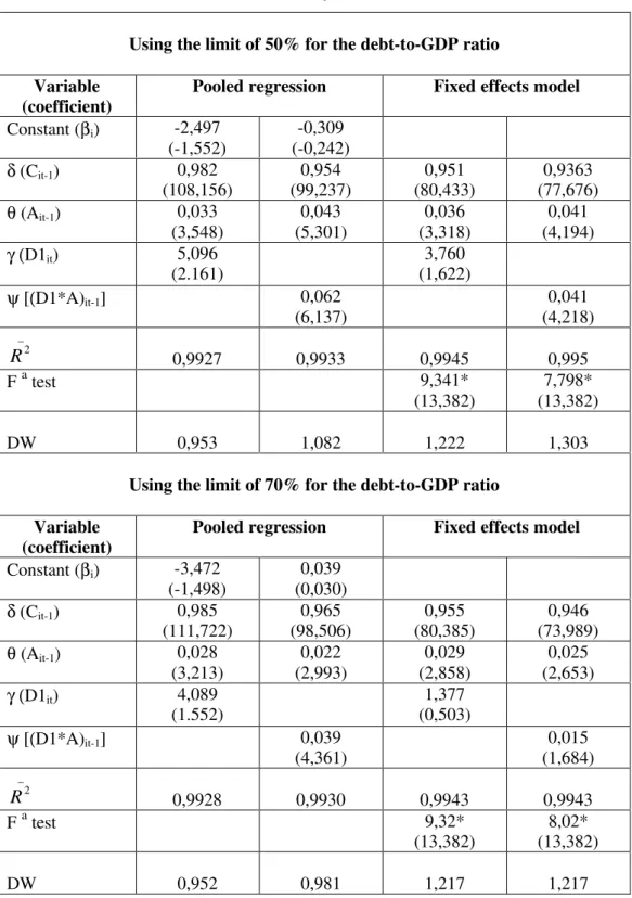
Since the 60 per cent limit for the debt-to-GDP ratio lacks a clear-cut economic rationalization, equations (10) e (11) where also estimated using as an alternative for the debt-to-GDP ratio, the 50 and the 70 per cent thresholds. The dummy variable D1 is once again computed for each country, in each year. The results of this new set of estimations are presented in Table 6.

16

Table 6 – Estimation of equations (10) and (11), dummy variable computed for

each year

Using the limit of 50% for the debt-to-GDP ratio

Variable (coefficient)

Pooled regression Fixed effects model

Constant (βi) -2,497

(-1,552)

-0,309 (-0,242)

δ (Cit-1) 0,982

(108,156) 0,954 (99,237) 0,951 (80,433) 0,9363 (77,676)

θ (Αit-1) 0,033

(3,548) 0,043 (5,301) 0,036 (3,318) 0,041 (4,194)

γ (D1it) 5,096

(2.161)

3,760 (1,622)

ψ [(D1*A)it-1] 0,062

(6,137)

0,041 (4,218)

_ 2

R 0,9927 0,9933 0,9945 0,995

F a test 9,341*

(13,382)

7,798* (13,382)

DW 0,953 1,082 1,222 1,303

Using the limit of 70% for the debt-to-GDP ratio

Variable (coefficient)

Pooled regression Fixed effects model

Constant (βi) -3,472

(-1,498)

0,039 (0,030)

δ (Cit-1) 0,985

(111,722) 0,965 (98,506) 0,955 (80,385) 0,946 (73,989)

θ (Αit-1) 0,028

(3,213) 0,022 (2,993) 0,029 (2,858) 0,025 (2,653)

γ (D1it) 4,089

(1.552)

1,377 (0,503)

ψ [(D1*A)it-1] 0,039

(4,361)

0,015 (1,684)

_ 2

R 0,9928 0,9930 0,9943 0,9943

F a test 9,32*

(13,382)

8,02* (13,382)

DW 0,952 0,981 1,217 1,217

The t statistics are in parentheses.

a - The degrees of freedom for the F statistic are in parentheses; the statistic tests the fixed effects model against the pooled regression model, where the autonomous term is the same for all countries, which is the null hypothesis.

These results can be compared with the ones obtained when the 60 per cent debt-to-GDP ratio was used (see Tables 3 and 4). Looking at for instance the fixed effects regression, with the multiplicative dummy variable, one can see that now the results are statistically more significant. In fact, with the 50 per cent limit, the coefficient (ψ) for the relevant exogenous variable is now unequivocally significant and positive. Also, the effect of a change in the stock of government debt, on private consumption, seems to be more substantial. Indeed, an increase of 1000 Euros has the effect of raising private consumption by 82 Euros (θ+ψ = 41+41 = 82) if government indebtedness is more mitigated, or may raise private consumption by 41 Euros when the debt-to-GDP is larger, and consumers depict in some way more Ricardian features.

Furthermore, when the 70 per cent limit for the debt-to-GDP ratio is used, the results are not statistically more significant than obtained with booth the 50 and the 60 per cent limits, even if the coefficients still have the right signs. Estimations were also made, with the thresholds of 50 and 70 per cent, but computing the D1 variable as the period average for each country. However, the results, not presented in the paper, did not improve the statistical quality of the estimated models. One must then also conclude that it is better to use, for the dummy variable, the values observed in each year for the debt-to-GDP, in every country.

It looks then as if above the 50 per cent threshold, consumers are somehow more aware of the future consequences of government indebtedness. In addition, the wealth variable now becomes more significant than in the specifications where the countries were labelled as “more” or “less” indebted according to the 60 per cent limit for the debt-to-GDP ratio. Briefly, with the 50 per cent limit for the debt-to-debt-to-GDP ratio, one cannot reject the hypothesis that public debt is relevant to explain private consumption, with this relation being a positive one.

5 - Conclusions

consumption response to government debt indebtedness, solely using the EU-15 countries. It is therefore implicit in the empirical analysis, the assumption that this set of countries has somehow certain common features, relating namely consumer’s behaviour throughout the EU.

Tentatively one could perhaps notice that private consumption is more responsive to wealth increases in “less indebted” countries than in the “more indebted” countries. Therefore, if we ask the question, does higher government indebtedness imply a more Ricardian behaviour from European consumers, a cautious answer would be that there seems to be some evidence pointing that way.

Also, estimations with different limits for the debt-to-GDP ratio, 50, 60 and 70 per cent, in order to assess a possible threshold for the change in consumers behaviour, seem to reveal that the 50 per cent limit provides a clearer consumer behaviour distinction according to the country indebtedness level.

Our results, for a data set that could in some way be considered as a smaller sample of the OECD countries, weigh against those of Evans (1993) in some way, since he does not reject the neutrality hypothesis for the OECD countries, and match up to those of Lopez et al. (2000) who reject the neutrality hypothesis for the OECD countries. The present paper uses however a different empirical approach vis-à-vis the cited papers.

Annex: Data sources

Public debt – national currency;

Budget deficit, general government – national currency, market prices; GDP – national currency, market prices;

Private consumption – national currency, market prices; Exchange rates – ECU, Euro, versus national currency;

source: European Economy, nº 71, European Commission, 2000.

Consumer Price Index – 1990 = 100,

References

Afonso, A. (1999). "Public Debt Neutrality and Private Consumption: some Evidence from the Euro Area," DGEP - Research and Forecasting Department, Ministry of Finance, Working Paper nº 11, June.

Afonso, A. and Teixeira, J. (1998). “Non-linear Tests of Weakly Efficient Markets: Evidence from Government Bond Markets in the Euro Area,” Cadernos do Mercado de Valores Mobiliários, 3, 2nd Semester.

Afonso, A. and St. Aubyn, M. (1999). “Credit Rationing and Monetary Transmission: Evidence for Portugal,” Estudos de Economia, XIX (1), 5-19.

Aschauer, D. (1985). “Fiscal Policy and Aggregate Demand,” The American Economic Review, 75 (1), March, 117-127.

Aschauer, D. (1988). “The Equilibrium Approach to Fiscal Policy,” Journal of Money, Credit and Banking, 20 (1), 41-62.

Barro, R. (1974). “Are Government Bonds Net Wealth?” Journal of Political Economy, 82 (6), 1095-117.

Barro, R. (1976). “Reply to Feldstein and Buchanan,” Journal of Political Economy, 84 (2), 343-349.

Barro, R. (1979). “On the Determination of Public Debt,” Journal of Political Economy, 87 (5), 940-971.

Barro, R. (1989). “The Ricardian Approach to Budget Deficits,”Journal of Economic Perspectives, 3 (2), 37-54.

Barro, R. (1998). "Reflections on Ricardian equivalence," in Maloney, J. (ed.), Debt and Deficits: an Historical Perspective, Edward Elgar Pub.

Bhargava, A.; Franzini, L. and Narendanathan, W. (1982). “Serial Correlation and the Fixed Effects Model,”Review of Economic Studies, 49 (4), 533-549.

Becker, G. (1974). “A theory of social interactions,” Journal of Political Economy, 82 (6), 1063-1093.

Bernheim, D. (1987). “Ricardian Equivalence: An Evaluation of Theory and Evidence,” in Fischer, S. (ed.), NBER Macroeconomics Annual 1987, Cambridge, Mass., MIT Press, 263-315.

Bernheim, D. (1989). “A Neoclassical Perspective on Budget Deficits,” Journal of Economic Perspectives, 3 (2), 55-72.

Blinder, A. and Solow, R. (1973). “Does Fiscal Policy Matter?” Journal of Public Economics, 2, 319-337.

Blinder, A. and Deaton, A. (1985). “The Time Series Consumption Function Revisited,” Brookings Papers on Economic Activity, 2, 465-521.

Brennan, H. and Buchanan, J. (1986). “The Logic of the Ricardian Equivalence Theorem,” in Buchanan, J; Rowley, C and Tollison, R. (eds), Deficits, Oxford, Basil Blackwell, 79-92.

Buchanan, J. (1976). “Barro on the Ricardian Equivalence Theorem,” Journal of Political Economy, 84 (2), 337-342.

Buiter, W. (1985). “A Guide to Public Sector and Deficits,” Economic Policy, 1, 13-79. Buiter, W. and Tobin, J. (1979). “Debt Neutrality: A Brief Review of Doctrine and Evidence” in von Furstenberg, G. (ed.), Social Security versus Private Saving, Cambridge, Mass., Ballinger, 39-63.

Carmichael, (1982). “On Barro's theorem of debt neutrality: the irrelevance of net wealth,” American Economic Review, 72 (1), 202-213.

Christ, C. (1978). “Some Dynamic Theory of Macroeconomic Policy Effects on Income and Prices under the Government Budget Restraint,” Journal of Monetary Economics, 4, 45-70.

Cushing, M. (1992). “Liquidity constraints and aggregate consumption behaviour,” Economic Inquiry, 30 (1), 134-53.

Dalamagas, B. (1992). “How Rival are the Ricardian Equivalence Proposition and the Fiscal Policy Potency View,” Scottish Journal of Political Economy, 39 (4), 457-476. Diamond, P. (1965). “National Debt in a Neoclassical Growth Model,” The American Economic Review, 60, 1126-1150.

Eisner, R. (1989). “Budget Deficits: Rhetoric and Reality,” Journal of Economic Perspectives, 3 (2), 73-93.

Elmendorf, D. e Mankiw, N. (1999). “Government Debt,” in Taylor, J. e Woodford, M. (eds.), Handbook of Macroeconomics, North-Holland Pub. Co.

Evans, P. (1988). “Are Consumers Ricardian? Evidence for the United States,” Journal of Political Economy, 96 (5), 983-1004.

Evans, P. (1993). “Consumers are not Ricardian: evidence from nineteen countries,” Economic Inquiry, 31, 534-548.

Greene, W. (1997). Econometric Analysis, 3ª ed., Prentice Hall.

Gupta, K. (1992). “Ricardian Equivalence and Crowding out in Asia,” Applied Economics, 24, 19-25.

Hall, R. (1978). “Stochastic Implications of the Life Cycle-Permanent Income Hypothesis: Theory and Evidence,” Journal of Political Economy, 86 (6), 971-987. Hausman, J. (1978). "Specification Tests in Econometrics," Econometrica, 46 (6), 1251-1271.

Hayashi, F. (1982). “The Permanent Income Hypothesis: Estimation and Testing by Instrument Variables,” Journal of Political Economy, 90 (5), 895-916.

Himarios, D. (1995). “Euler Equation Tests of Ricardian Equivalence,” Economics Letters, 48, 165-171.

Jaffee, D. and Russell, T. (1976). “Imperfect information, uncertainty, and credit rationing,” Quarterly Journal of Economics, 4, 651-666.

Johnston, J. e DiNardo, J. (1997). Econometric Methods, 4ª ed., McGrawHill.

Judson, R. e Owen, A. (1997). “Estimating Dynamic Panel Data Models: A Practical Guide for Macroeconomists,” Finance and Economics Discussion Papers 1997-3, Federal Reserve System.

Khalid, A. (1996). "Ricardian Equivalence: Empirical evidence from developing economies," Journal of Development Economics, 51 (2), 413-432.

Leiderman, L. and Razin, A. (1988). “Testing Ricardian Neutrality with an Intertemporal Stochastic Model,” Journal of Money, Credit and Banking, 20 (1), 1-21. Lopez, J.; Schmidt-Hebbel, K. e Servén, L. (2000). "How effective is fiscal policy in raising national saving?" Review of Economics and Statistics, 82 (2), 226-238.

O’Driscoll, G. P. (1977). “The Ricardian Nonequivalence Theorem,” Journal of Political Economy, 85 (1), 207-210.

Phelps, E. (1982). “Cracks on the Demand Side: A Year of Crisis in theoretical Macroeconomics,” American Economic Review, 72 (2), 378-381.

Ricardo, D. (1817). On the Principles of Political Economy and Taxation, in P. Sraffa (ed.), The works and correspondence of David Ricardo, Volume I, 1951, Cambridge University Press, Cambridge.

Ricardo, D. (1820). Funding System, in P. Sraffa (ed.), The works and correspondence of David Ricardo, Volume IV, 1951, Cambridge University Press, Cambridge.

Rose, D. and Hakes, D. (1995). “Deficits and Interest Rates as Evidence of Ricardian Equivalence,” Eastern Economic Journal, 21 (1), 57-66.

Samuelson, P. (1958). “An Exact Consumption-Loan Model of Interest with or without the Social Contrivance of Money,” Journal of Political Economy, 66 (6), 467-482. Seater, J. (1993). “Ricardian Equivalence,” Journal of Economic Literature, XXXI, March, 142-190.

Sims, C. (1998). “Econometric implications of the government budget constraint,” Journal of Econometrics, 83 (1-2), 9-19.

Stiglitz, J. and Weiss, A (1991). “Credit rationing in markets with imperfect information,” The American Economic Review, 71, 393-411.