Universidade de Lisboa
Faculdade de Farmácia
A quality-by-design approach for the
understanding of the effect of model antigen
on mannose PLGA nanoparticles
Ainhoa Teresa Cardoso Coelho
Mestrado Integrado em Ciências Farmacêuticas
Universidade de Lisboa
Faculdade de Farmácia
A quality-by-design approach for the
understanding of the effect of model antigen
mannose on PLGA nanoparticles
Ainhoa Teresa Cardoso Coelho
Monografia de Mestrado Integrado em Ciências Farmacêuticas apresentada à
Universidade de Lisboa através da Faculdade de Farmácia
Orientador: Professor Doutor João Almeida Lopes
iii
Resumo
A incidência do melanoma tem aumentado relativamente à maioria dos cancros. A redução da sua incidência através de métodos que permitam uma deteção precoce e prevenção do melanoma são da responsabilidade dos profissionais de saúde. As formas tradicionais de tratamento demonstram efeitos secundários muito graves e não atacam somente as células tumorais. Portanto, são necessárias novas estratégias terapêuticas, como as vacinas terapêuticas baseadas em nanopartículas, desenvolvidas tendo em vista o transporte de antigénios tumorais e adjuvantes para células apresentadoras de antigénios, como as células dendríticas.
Nanopartículas de poli(ácido láctico-co-glicólico) (PLGA) que têm como ligando um recetor de manose à superfície das células apresentadoras de antigénio, álcool polivinílico ou d-α-tocoferil polietileno glicólico 1000 sucinato como tensioativos e PLGA conjugado com cianina 5,5, foram preparadas por dupla emulsão seguida de evaporação de solvente. Com vista a modificar as caraterísticas físico-químicas das nanopartículas, foram feitas variações na quantidade de manose incorporada. Estas nanopartículas de PLGA funcionalizadas com manose foram investigadas ao nível das suas caraterísticas (tamanho médio, carga superficial e índice de polidispersão) e células dendríticas foram tratadas com estas nanopartículas para avaliação da intensidade da fluorescência. Implementar o conceito de quality-by-design para o desenvolvimento das nanopartículas assegura que a qualidade é mantida. O tamanho médio e o índice de polidispersão foram avaliados por espalhamento dinâmico da luz e o potencial zeta foi determinado por velocimetria laser. O tamanho médio das nanopartículas variaram entre 184,6 a 194,0 nm e a carga superficial entre 2,51 a -1,09 mV. A intensidade de fluorescência média foi medida por citometria de fluxo. Para um melhor entendimento dos parâmetros de processo críticos e dos atributos de qualidade críticos, foi usado um modelo matemático linear. Fator e respostas foram determinados. Um modelo causal preditivo mostrou a importância de todos os fatores e das interações estabelecidas.
Palavras-chave: nanopartículas; poli(ácido lático-co-glicólico); ácido poliláctico;
Abstract
The incidence of melanoma is increasing at a faster rate than almost all other cancers. The reduction of this incidence through better methods of early detection and prevention of melanoma will be the responsibility of clinicians. Conventional forms of treatment demonstrate severe side effects and do not target tumour cells. Thus, there is a need for new therapeutic strategies. In this context, nanoparticle-based therapeutic vaccine, which target tumour cells and are immunotherapeutic appear as a promising alternative.
Poly (lactic-co-glycolic acid) nanoparticles which bind as a mannose receptor to the surface of the antigen-presenting cells, polyvinyl alcohol or d-α-tocopheryl polyethylene glycol 1000 succinate and labelled with cyanine5.5 carboxilic acid were prepared by double emulsion with solvent evaporation technique. To modify physicochemical characteristics of nanoparticles, variations were made in the amount of incorporated mannose. These mannose functionalized PLGA nanoparticles were investigated for their characteristics and the dendritic cells treated with these nanoparticles were evaluated for fluorescence intensity. Implementing the quality-by-design approach for the development of NPs ensures that quality is sustained. Average size and polydispersity index were assessed by dynamic light scattering and zeta potential was determined by laser doppler velocimetry. Nanoparticle Z-ave varied from 184.6 to 194.0 nm and surface charge varied from -2.51 and -1.09 mV. Median fluorescence intensity was measured by flow cytometry. For better understanding of critical process parameters and critical quality attributes, a mathematical linear modelling approach was used. Factor and responses were determined. A causal predictive model showing the importance of all factors and their interactions was established.
Key words: nanoparticles; poly(lactic-co-glycolic acid); polylactic acid;
v
Acknowledgements
This dissertation represents the culmination of a journey. A path not always easy. However, I want to thank all the people who have supported me. They have made me the person I am today.
At first, I want to thank to Professor Helena Florindo for teaching and guiding me in the redaction of this report. My special thanks go for Carina Peres, who accompanied my work very closely and gave me the orientation I needed.
Secondly, I express my deepest gratitude to my supervisor, Professor João Lopes, not only for the opportunity to develop this and other projects, but also for the unconditional help, support and friendship throughout this years.
Also, I want to express my thanks to my long-time friends who, despite the distance, have kept by my side and the friendships I made during college.
To my family, especially to my mother, I present my biggest gratitude, for always leaning on my hardest moments, for the constant dedication and protection, for encouraging me since I was little to have a higher education, for all the efforts made and all that has abdicated for me.
List of Abbreviations
APC – Antigen-Presenting Cell ANOVA – Analysis of Variance Cy5.5 – Cyanine5.5 Carboxilic Acid DCC – Carbodiimide
DCM – Dichloromethane
DLS – Dynamic Light Scattering DMAP – 4-(Dimethylamino) Piridine DMF – Dimethylformamide
DMSO – Dimethyl Sulfoxide DoE – Design of Experiment FBS – Fetal Bovine Serum
FDA – Food and Drug Administration FI – Fluorescence Intensity
LDV – Laser Doppler Velocimetry Man – Mannose
Mn – Number Average of Molecular Weight
Mw –Molecular Weight
MVA – Multivariate Analysis
MWD – Molecular Weight Distribution NPs – Nanoparticles
PBS – Phosphate-buffered Saline PAT– Process Analytical Technology PC – Principal Component
PCA – Principal Component Analysis PdI – Polydispersity Index
pH – Potential of Hydrogen PLA – Polylactic acid
PLGA – Poly (lactic-co-glycolic acid) PVA – Polyvinyl Alcohol
QbD – Quality-by-design QCA – Quality critical attributes RER – Ranger Error Ratio R2
CAL – Coefficient of Determination in Calibration
vii
RMSEC – Root Mean Square Error of Calibration
RMSECV – Root Mean Square Error of Cross Validation RMSEP – Root Mean Square Error of Prediction
SECV – Standard Error of Cross Validation SEEDS – Self Emulsifying Drug Delivery System Tg – Glass-transition Temperature
TPGS – d-α-Tocopheryl Polyethylene Glycol 1000 Succinate Z-ave – Average Size
Table of Contents Resumo ... iii Abstract ... iv List of Abbreviations ... vi List of Figures ... x List of Tables ... xi
List of Equations ... xii
1. Introduction ... 1
1.1. Cancer ... 1
1.1.1. Characterisation, epidemiology and causes ... 1
1.1.2. Diagnosis and treatment ... 1
1.1.2.1. Cancer vaccines ... 1 1.2. Nanoparticles ... 2 1.2.1. Nanopsheres ... 2 1.2.2. Formulation methodology ... 2 1.3. Raw Materials ... 3 1.3.1. Polyvinyl alcohol ... 3 1.3.2. Polylactic-co-glycolic acid ... 3
1.3.3. d-α-Tocopheryl Polyethylene Glycol 1000 Succinate ... 4
1.3.4. Poly (lactic acid) ... 4
1.3.5. Mannose ... 5
1.3.6. Cyanine5.5 carboxilic acid ... 5
1.4. Nanoparticles characterization ... 6 1.4.1. Zeta potential ... 6 1.4.2. Average size ... 6 1.4.3. Polydispersity index ... 7 1.5. Fluorescence intensity ... 7 1.6. Quality by design ... 8 1.6.1. Multivariate analysis ... 10
ix
1.6.1.1. Unsupervised analysis ... 10
1.6.1.2. Supervised approach ... 11
2. Literature review ... 13
3. Objective... 14
4. Materials and methods ... 14
4.1. Materials ... 14
4.2. Methods ... 15
4.2.1. Preparation of polymeric nanoparticles ... 15
4.2.2. Physicochemical characterisation of NPs ... 16
4.2.2.1. Size and polydispersity index ... 16
4.2.2.2. Zeta potential ... 16
4.2.3. Fluorescence intensity ... 17
5. Results and discussion ... 17
5.1. Physicochemical characterisation of nanoparticles ... 17
5.2. Fluorescence intensity ... 17 5.3. Multivariate Analysis ... 20 5.3.1. Analysis of Variance ... 20 5.3.2. PCA modelling ... 20 5.3.3. Prediction ... 22 6. Conclusion ... 25 7. References ... 26
List of Figures
Figure 1. Schematic representation of the structure of a nanosphere ... 2
Figure 2. General structure of PVA ... 3
Figure 3. General structure of PLGA ... 4
Figure 4. General structure of TPGS ... 4
Figure 5. General structure of PLA ... 4
Figure 6. General formula of mannose ... 5
Figure 7. General structure of Cy5.5 ... 5
Figure 8. Absorption and emission spectra of Cy5.5 fluorophore ... 6
Figure 9. Schematic representation of a hydrodynamic focusing of the sample core through the flow cell of BD LSR Fortessa™ ... 8
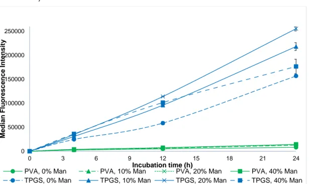
Figure 10. Median fluorescence intensity of NPs prepared with TPGS and PVA with different quantities of mannose (0%, 10%, 20% and 40%) ... 18
Figure 11. Median intensity fluorescence of NPs prepared with PVA with different quantities of mannose (0%, 10%, 20% and 40%) ... 19
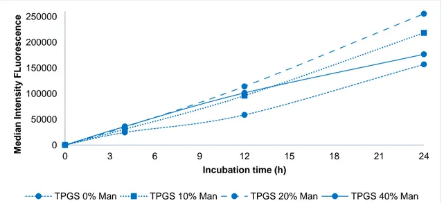
Figure 12. Median intensity fluorescence of nanoparticles prepared with TPGS with different quantities of mannose (0%, 10%, 20% and 40%) ... 19
Figure 13. Results of principal component analysis of fluorescence intensity (FI), polydispersity index (PdI), average size (Z-Ave), zeta potential (ZP), PVA-Mannose 0, 10, 20, 40% and TPGS-Mannose 0,10, 20, 40% ... 21
Figure 14. PCA model loadings for the first two principal components: average size (Z-Ave), polydispersity index (PdI), zeta potential (ZP) and fluorescence intensity (FI) at 4h, 12h and 24h. ... 22
xi
List of Tables
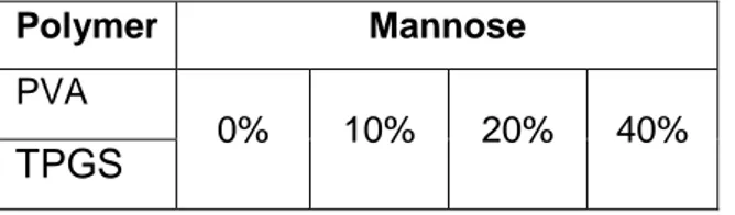
Table 1. Percentage of mannose on the formulations with PVA and TPGS ... 16
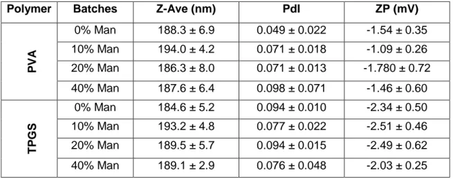
Table 2. Mean values of mean diameter (Z-Ave), PdI and surface charge (ZP) (mean ± SD; n=3) ... 17
Table 3. Median fluorescence intensity of NPs prepared with PVA and TPGS with 0%, 10%, 20% and 40% of mannose ... 18
Table 4. ANOVA for the type of polymer ... 20
Table 5. ANOVA for the mannose content ... 20
Table 6. Summary of the MLR models for the six evaluated parameters. ... 23
Table 7. Root mean square of error prediction of model predictions (cross validation) 23 Table 8. Percentage error of model predictions (cross validation) ... 24
Table 9. Standard error of model predictions (cross validation) ... 24
Table 10. Regression coefficients for the developed MLR models. ... 25
List of Equations
Equation 1. Definition of the polydispersity index ... 7 Equation 2. Definition of the root-mean-square error ... 12
1
1. Introduction
1.1.
Cancer
1.1.1. Characterisation, epidemiology and causes
Cancer is a heterogenous disease that results from a multi-step process, characterized by uncontrolled tumour cell growth, invasion and metastasis. Tumour cells have also the ability to evade cell death1 and to escape immune system
surveillance.2 There are three general classifications of neoplasia: epithelial neoplasia;
mesenchymal, neuroendocrine and germ cell neoplasia; and hematologic neoplasia. The malignant potential of these cells is related to the proliferative rate and perhaps to exposure to environmental, dietary, and endogenous hormonal or growth factor stimuli.3
1.1.2. Diagnosis and treatment
Radiotherapy, chemotherapy, immunotherapy and surgery are some strategies for cancer treatment.4 Many of these procedures are unspecific with severe side effects.5
Those single treatment regimens have limited chances to eradicate cancer cells in a permanent way due to their heterogeneous nature.6 Despite developments in diagnosis
and therapies, 11.5 million deaths are predicted for cancer in 2030. The success of cancer therapy depends on the development of other strategies to overcome severe side effects, drug resistance and circumvent tumour evasion mechanisms.7
The immune system has a significant role in controlling malignant cells’ growth. It can respond against tumours and this effect can be improved using several strategies.8
The specificity of the immune system is used on cancer immunotherapy approach and provides a more efficacious and better tolerated treatment than the conventional ones. Enhancement of host’s own immune response to a tumour is the objective of the new approaches to cancer immunotherapy, such as prophylactic and therapeutic cancer vaccines, cytokine therapy, administration of immune activating antibodies and radioimmunotherapy.9
1.1.2.1. Cancer vaccines
Nanoparticles (NPs) enable the generation of an effective immune response thanks to their unique capacity for targeting the immune system and co-delivering antigen and adjuvant to the same cell at the same time.10 The selection of the
appropriate tumour antigens is a major obstacle to the development of efficacious cancer vaccines.11 This type of vaccines would be administered after the beginning or
immune response must be taken into account while designing cancer vaccines. This will successfully improve patient defences against the malignant cells and also overcome the mechanisms of tumour evasion and tolerance.12 The presence of the
antigen in a variety of tumour tissues and the role of this antigen in tumour growth and metastasis should be the base of the selection of a cancer vaccine target antigen. The use of aliphatic polyesters to formulate biodegradable polymeric NPs have a long history of use for biomedical applications. The aliphatic polyesters used in this experiment are poly (lactic-acid) (PLA) and Poly (lactic-co-glycolic acid) (PLGA).
1.2.
Nanoparticles
1.2.1. Nanopsheres
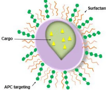
The most common NPs are micro/nanospheres, micro/nanocapsules, polymeric micelles and nanogels.13 The particulate vaccine delivery system formulated in this
experiment was a nanosphere, represented in figure 1. The nanosphere, called nanoparticle to simplify, is a nanoparticle composed by a polymeric matrix in which the cargo is dispersed.14 There are major challenges in the preparation of NPs, due to
absence of understanding of the effect of critical material attributes and critical processing parameters to achieve small size and low PdI. Nanoparticulate drug delivery system is also recognised for its the fast onset action, increase in solubility, permeability, and bioavailability.15
Figure 1. Schematic representation of the structure of a nanosphere
1.2.2. Formulation methodology
NPs may be prepared by different methods. The most often adopted techniques are solvent evaporation (single or multiple emulsion), solvent extraction process (single
3
or multiple emulsion), phase separation, spray-drying and dialysis.16 The method used
in this work was the double emulsion water-in-oil-in-water (W/O/W) solvent evaporation technique. This method allows the production of W/O/W nano-emulsions that originate NPs suspensions after the evaporation of organic phase. More detailed, this technique permits the encapsulation of hydrophilic drugs, such as nucleic acids, peptides and proteins. The emulsion is prepared by adding water and surfactants to the polymer solution. The nanosized droplets are induced by sonication or homogenization, in this case was used the first technique. Then, the solvent is evaporated or extracted and the NPs collected after centrifugation.17 The great stability of droplet suspension and
absence of the flocculation phenomenon is the main particularity of nano-emulsions.18
1.3.
Raw Materials
1.3.1. Polyvinyl alcohol
Polyvinyl alcohol (PVA) with the linear formula [-CH2CHOH-]n and the general
formula represented in figure 2 is used as a surfactant, thus stabilizing the nano-emulsion. This product has Mw of 13 000- 23 000 g/mol, is presented in the forms of
powder, crystalline powder, crystals or granules and 87-89% is hydrolysed.19
Figure 2. General structure of PVA
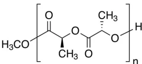
1.3.2. Polylactic-co-glycolic acid
Polylactic-co-glycolic acid with the linear formula [C3H4O2]x[C2H2O2]y and
structural formula demonstrate in figure 3, The composition of PLGA can be fine tune according to the desired degradation rate. In this experiment, PLGA 50:50 was used, that is 50% lactic acid and 50% glycolic acid. This polymer is hydrophilic and has the fastest biodegradation rate of PLGA polymers.20 One of the most used biodegradable
polymers is PLGA, because its hydrolysis leads to metabolite monomers, lactic acid and glycolic acid. These two monomers are endogenous and simply metabolized via the Krebs cycle, so a minimal systemic toxicity is associated to the use of this polymer.21 PLGA NPs have been efficaciously formulated to encapsulate a variety of
Figure 3. General structure of PLGA
1.3.3. d-α-Tocopheryl Polyethylene Glycol 1000 Succinate
d-α-Tocopheryl Polyethylene Glycol 1000 Succinate (TPGS) represented in figure 4 with the empirical formula C33O5H54(CH2CH2O)n is used as a source of natural
vitamin E. It also has shown properties to improve bioavailability of poorly absorbed drugs vitamins micro-nutrients acting as an absorption and permeability enhancer and to develop self-emulsifying drug delivery system (SEEDS) for poorly soluble drugs as an emulsifier. α-tocopherol may be used to create biodegradable polymers and antioxidant surfactants. The melting point of TPGS is superior to 36ºC, it is soluble in water, has a Mw approximately of 1513 g/mol and a storage temperature between
2-8ºC.23
Figure 4. General structure of TPGS
1.3.4. Poly (lactic acid)
Poly (lactic acid) (PLA) represented in figure 5 with the empirical formula [-OCH(CH3)CO-]n is a biodegradable polymer for medical device and pharmaceutical
applications. It is used to fabricate resorbable medical devices that degrade over months in physiological conditions. PLA has also been used to a lesser extent than PLGA due to the lower degradation rate.24
5
1.3.5. Mannose
Mannose with the empirical formula C6H12O6 is in figure 6 and has Mw of 180.16
g/mol. Man is a natural monosaccharide that can be obtained both by plants and microorganisms. The melting temperature is 132ºC and is easily soluble in water and slightly soluble in ethanol.25 In this experiment, mannose was used to increase the
recognition and internalization of NPs by dendritic cells.
Figure 6. General formula of mannose
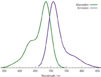
1.3.6. Cyanine5.5 carboxilic acid
Cyanine5.5 carboxilic acid (Cy5.5) has the molecular formula C40H43N2O2+ and
Mw of 583.796 g/mol represented in figure 7. This compound is soluble in organic
solvents (dimethyl sulfoxide (DMSO), dichloromethane (DCM), dimethylformamide (DMF) and possess low solubility in water. Cy5.5 must be stored at -20ºC in the dark for 24 months and avoid prolonged exposure to light. Cy5.5 has also fluorescent properties, with an excitation maximum at 684 nm and an emission maximum at 710 nm (figure 8).26
Wavelength (nm)
Figure 8. Absorption and emission spectra of Cy5.5 fluorophore
1.4.
Nanoparticles characterization
1.4.1. Zeta potential
Surface charge of NPs may have an important control on their biodistribution following i.v. injection. Neutral charge interacts minimally with plasma proteins and thus contributes to the extended circulation time of the NPs, whereas a high surface charge (negative or positive) enhances the phagocytosis process.27 The chemical properties of
the polymer, the stabilizing agent and pH of the dispersant are factors dependent on the polymeric particle charge. Surface charge measures the efficiency of surface modification and has a vast effect on internalization capability. One method involves the determination of the zeta potential (ζ or ZP) of the NPs via the movement of charged particles monitored by an electrical potential. The ZP values may be positive, neutral or negative, depending on the polymer used and the surface modification.28 The
ionic interactions established between positively charged particles and the negatively charged cell membrane result on a higher extent of internalization of positively charged NPs. Negatively charged copolymers are associated to a slow uptake, whereas fast and efficient uptake is associated with positively charged copolymers due to non-specific adsorptive.29
1.4.2. Average size
The size of the NPs is one of the important parameters influencing the pharmacokinetic and biodistribution of the intravenously injected NPs. The uptake of particulate vaccines by APCs and the determination of their intracellular fate are affected by size. The thermodynamic driving force and the receptor driving force are
7
and the time needed for that.30 The average size (Z-ave) can be measured by photon
correlation spectroscopy (dynamic light scattering). This method is based on the Brownian motion of the particles that cause dispersion of the light. The information on the morphology and size of the NPs are provided by imaging techniques. Normally, the Z-ave of the NPs is in the range of 100 to 250 nm.31 Some studies revealed that NPs
smaller than 50 nm tend to aggregate during cellular uptake 32 and the ones larger than
approximately 55 nm would have the fastest wrapping time and could produce enough free energy to drive the NPs into the cell.33 NPs size cannot be ignored when
considering the route of administration of the vaccine.34
1.4.3. Polydispersity index
PdI is the ratio of the molecular weight averages (heterogeneity ratio, dispersion ratio, non-uniformity coefficient), used for description of the polymer molecular weight distributions (equation 1) and can be measured by dynamic light scattering (DLS), as explained in the previous section. This parameter is calculated from a Cumulants analysis of the DL-measured intensity autocorrelation function. The PdI is often taken as the absolute measure of the molecular weight distribution (MWD), while some objections have been presented to confront that opinion.35 PdI is dimensionless and
scaled such that values smaller than 0.05 are rarely seen other than with monodisperse standards. Values greater than 0.7 indicate that the sample has a very broad size distribution and is probable not suitable for the DLS technique. The larger PdI, the broader the MWD. Nevertheless, widely accepted belief, the reverse is not true. Therefore, the increase in the MWD width is automatically interpreted in terms of the increase in the PdI. However, a very simple simulation of the MWD can evidently confirm the possible existence of distributions with large differences in width, but with unique PdI.36
Polydispersity index =Mw Mn
Equation 1. Definition of the polydispersity index
1.5.
Fluorescence intensity
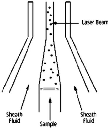
The principle of fluorescence intensity (FI) is the movement of resuspended single cells through a light source, commonly a laser. The FI is proportional to the amount of light absorbed and the fluorescence quantum yield. In this process cells emit light signals depending on the cell type and the preparation of cells that are detected by appropriate detectors. FI is measured by flow cytometry and a flow cytometer need a fluidic (moves and aligns cells into the laser focus), optical (excitation and detection optics) and electronical (transfers optical signals into electronical signals, digitalizes the
electronical signals for the analysis on a computer) systems. For these measurements, the optical system illuminates the sample using a specific wavelength (selected by an optical filter, or a monochromator), thereby exciting the sample. The excitation causes the sample to emit light (i.e. fluoresce) at a different wavelength. The emitted light is collected by a second optical system (emission system) and the signal is measured by a light detector.37 The equipment used in this research was BD LSR Fortessa™ and
the sample can be analysed at low pressure (12µL/min) or at high pressure (60µL/min). The lasers used were ‘‘blue’’ (488 nm), ‘‘red’’ (633 nm) and ‘‘violet’’ (405 nm). The detector has a octagon configuration.38
Figure 9. Schematic representation of a hydrodynamic focusing of the sample core through the flow cell of BD LSR Fortessa™
1.6.
Quality by design
Quality by design (QbD) have a key element that are product and process understanding. Design of experiment (DoE) is an exceptional tool to achieve these objectives that allows pharmaceutical scientists to systematically manipulate factors according to a pre-specified design. DoE reveals associations between input variables and outputs responses. DoE, when applied to formulation or process development, the input factors include the material attributes of raw material or excipients and process parameters whereas outputs remain the critical quality attributes of the in-process materials or final drug product.39
QbD has been applied within the pharmaceutical companies in the last few years. Pharmaceutical QbD have predefined purposes, highlights product, process understanding, control and quality risk management. Risk-based approaches and the implementation of QbD principles in drug product development, manufacturing, and regulation are encouraged by the Food and Drug Administration (FDA). Over the years, pharmaceutical QbD has evolved with the issuance of pharmaceutical development
9
Q10)42 and more recently, development and manufacture of drug substance (ICH
Q11)43. Product design, understanding, and control are equally important. The
objectives of pharmaceutical QbD are:
1. to accomplish expressive product quality specifications that are based on clinical performance;
2. to enhance product and process design, understanding and control by increasing process capability and diminish product variability and defects;
3. to increase product manufacturing and development efficiencies and 4. to highlight root cause analysis and post approval variation
management.
QbD consists of several elements, among which stand out:
1. the critical quality attributes of the drug product identified by the quality target product profile;
2. product design and understanding and identification of critical material attributes;
3. process design and understanding plus the identification of critical process parameters and thorough understanding of scale-up principles; 4. a control tactic that contains specifications for the active ingredient(s)
and excipient(s) as controls for each step of the manufacturing process and
5. process capability and continual enhancement.
To design and develop a robust drug product it is necessary to give earnest consideration to the biological, chemical, and physical properties of the drug substance. Excipients can be a major source of variability and alter the bioavailability, manufacturability and stability of drug products. To facilitate the early prediction of compatibility, the ICH Q8 guideline recommends drug-excipient compatibility studies. Formulation optimization studies are crucial in developing a robust formulation, without this is unknown whether any changes in the formulation itself or in the raw material properties would significantly impact the quality and performance of the drug product.44
Pharmaceutical products are commonly manufactured by a series of unit operations to produce the desired quality product. These operations may be executed in batch mode or in a continuous manufacturing process.45 Development studies
culminate in the establishment of a control strategy that could include three levels of controls (level 1, 2 and 3). Process capability measures process development through continuous improvement efforts that focus on eliminating sources of intrinsic variability from the process conditions and raw material quality. A set of activities that the
applicant carries out to improve its capability to meet requirements corresponds to continuous improvement. This can apply to legacy products.46
Process analytical technology (PAT) is applied to be part of the control strategy and ensures that the process remains within an established design space. The application of PAT includes four key components: multivariate data acquisition and analysis, process analytical chemistry tools, process monitoring and control and continuous process optimization and knowledge management.47 Principal component
analysis (PCA) is possibly the most widespread multivariate statistical technique. PCA analyses a data table representing observations labelled by numerous dependent variables inter-correlated. The objectives of PCA are the extraction of the most important information from the data table, compressing the size of the data by keeping only significant information, simplification of the description of the data set and analysing the structure of the observations and the variables.48
1.6.1. Multivariate analysis
Multivariate statistics studies the relationship between multiple measurements observed on a subject and predictive variable. MVA can be as simple as analysing two variables right up to millions. A multivariate model can show the influence that both types of variability can have on a system so that it can be better understood or improvements can be made. Multivariate data analysis is used for several distinct purposes, which are defined as 1) data description (explorative data structure modelling), 2) discrimination and classification and 3) regression and prediction. It is often necessary to sample, observe, study or measure more than one variable simultaneously. When we cannot measure or observe a desired parameter or variable directly, we are forced to turn to indirect observations, which is the situation in which multivariate data is most often generated. There must be a quantitative relationship between the set of measured variables and the property of interest. If the measurement variables change, the value of the indirect property must change consequently.49
Unsupervised/ supervised division are approaches to practical multivariate data analysis described below.
1.6.1.1. Unsupervised analysis
Unsupervised analysis is used for unsupervised purposes. It can perform an unsupervised data analysis when we do not know any specific data analysis purpose, like regression or classification, from the original problem specification.
Discriminative clustering is an unsupervised learning framework, which introduces the discriminative learning rule of supervised classification into clustering. The underlying assumption is that a good partition (clustering) of the data should yield
11
high discrimination, namely, the partitioned data can be easily classified by some classification algorithms. Clustering analysis has been widely used in many fields mainly for exploratory data analysis or class novelty discovery. Clustering analysis is also called unsupervised learning that includes classification and regression.
PCA is a statistical technique for determining key features of high dimensional dataset to simplify analysis. Recently, it has been explored as a method for clustering analysis, as it is fast and can handle large datasets. The objective of PCA is to substitute the representation of the objects, from the initial representation on the form of the p original variables into the new principal component coordinate space. The PCA performs a dual objective: a transformation into a more relevant co-ordinate system (which lies directly in the centre of the data swarm of the points), and a dimensionality reduction (using only the first principal components which reflect the structure in the data).50
1.6.1.2. Supervised approach
Supervised methods are used for supervised pattern recognition purposes. Supervised methods always comprise a two-stage process: 1) establishing a model for the X X or X Y relationship (e.g., PCR, PLS, MLR). This is called the calibration stage. This stage can in some sense be considered as a passive modelling stage, because the data themselves pretty much determines the model and 2) using this model for whatever purpose your original objective dictates for prediction for PCR, PLS, MLR, or for classification. This may be called the active stage, the classification or the prediction stage.
The validity and efficiency of any supervised data analysis method is totally dependent on the representativity of the initial data relationship used as a training basis. It is the responsibility of the data analyst to specify the training data set in an as relevant and representative manner as possible. Data classes and the samples therein must be representative with respect to future sampling of the populations modelled by the particular supervised method employed for the specific problem.51
MLR regression suffers from two different problems: 1) the relative abundance of response variables relative to the number of available calibration samples (for the typical spectral calibration problem), which leads to an underdetermined situation, and 2) the possibility of collinearity of the response variables in X, which leads to unstable matrix inversions and unstable regression results. PCR is one way to deal with both of these problems. Furthermore, the underdetermined problem in MLR is addressed by the fact that the maximum possible number of principal components (PCs) is equal to the lesser of the number of response variables and the number of calibration samples,
and, as a result, can never be greater than the number of calibration samples. Because it directly addresses the collinearity problem, PCR can be said to be less susceptible to overfitting than MLR. However, one could still overfit a PCR model through the retention of too many PCs. Therefore, as in PCA, an important part of PCR is the determination of the optimal number of principal components to retain in the model. In contrast to a PCA model, however, the purpose of a PCR regression model is to predict the properties of interest for new samples. As a result, we would like to determine the number of PCs that optimizes the predictive ability of the model. The appropriate number of PCs is typically determined by cross-validation, which involves a procedure where the available data are split sample-wise into training and a test set. The prediction residual error on the test set samples is then determined as a function of the number of PCs retained in the PCR model. This procedure is usually repeated several times, using different sample subset selections for training and test sets, such that each sample in the original data set is part of a test set at least once. We must also decide how to select the test sets for each repetition of the cross-validation procedure. Partial Least Squares (PLS) regression is related to both PCR and MLR, and can be thought of as occupying a middle ground between them. PCR finds factors that capture the greatest amount of variance in the predictor (X) variables. PLS attempts to find factors which both capture variance and achieve correlation. We commonly say that PLS attempts to maximize covariance. The PLS model is a basic tool widely used in chemometrics. The objective of this MVA statistical technique used to develop regression models is to establish a model for the analysis of unknown samples.52 Before comparing the predictive ability of the models, it is useful to review
several quality measures. In all of the measures considered, we are attempting to estimate the average deviation of the model from the data. R-squared (coefficient of multiple determination) describes how well the data points fit the statistical model (the line of regression). Values range from 0 to 1. A 100% accurate model would have an R-squared of 1 with all samples lying on the regression line. The root-mean-square error (RMSE) – seen in equation 2 – tells us about the fit of the model to the calibration data. 𝑅𝑀𝑆𝐸 = √∑ (𝑦̂ − 𝑦𝑖 𝑖) 2 𝑛 𝑖=1 𝑛
Equation 2. Definition of the root-mean-square error
In Eq. 2, ŷi are the values of the predicted variable when all samples are
13
measure of how well the model fits the data. The model is considered good when the value of RMSE is close to zero. The range error ratio (RER) is equal to the range in the compositional values (i.e. the maximum value minus the minimum value) divided by the RMSEP. The model is considered good when the value of RER is up to ten. The RER value can be compared with the RER value of other models, on the contrary the RMSE value cannot be compared.53
2. Literature review
The implementation of the concepts described in the ICH-Q8 guideline for the manufacturing of NPs for drug delivery are still limited. Unlike the adoption of this guideline for manufacturing of bulk products the situation for complex biologics especially those involving highly structured complex products do require a lot of research in the near future. Nonetheless, it is possible to find in the literature some research papers on the implementation of the QbD pharmaceutical development paradigm (involving its associated tools such as experimental design) for the development of nanoparticulate systems. Silva et al. (2015) demonstrated that the properties of NPs in terms of targeting and antigen/adjuvant delivery have high cancer immunotherapeutic potential.54They highlighted in another study the role of particulate
delivery systems composed by synthetic aliphatic polyesters on the field of vaccinology.55
McCall et al. (2013) studied the use of PLGA NPs via single or double emulsion using the emulsifying agent TPGS and characterized them.56
Yerlikaya et al. (2013) implemented a QbD approach for the development and characterization of paclitaxel NPs, identification and controlling critical sources of variability in the process, and understanding the impact of formulation and process parameters on the critical quality attributes (CQAs). This study demonstrated how the understanding of formulation and process parameters is useful for the optimization of complex drug delivery systems.57
Dongmei Cun et al. (2011) defined optimal parameters for the preparation of small interfering RNA (siRNA)-loaded PLGA NPs by the double emulsion solvent evaporation method and characterized the NPs properties. The results of this study enabled careful understanding and definition of optimal process parameters for preparation of PLGA NPs encapsulating high amounts of siRNA with immediate and long-term sustained release properties.58
Rahman et al. (2011) modelled the product variability due to important factors affecting CyA-PLGA NPs prepared by O/W emulsification-solvent evaporation method.
Independent variables studied were cyclosporine A (CyA) (X1), PLGA (X2), and
emulsifier concentration namely SLS (X3), stirring rate (X4), type of organic solvent
employed (chloroform or dichloromethane, X5) and organic to aqueous phase ratio (X6).
This study revealed the potential of QbD strategy for optimising a formulation through the deep understanding of the effect of formulation and process variables on the characteristics on CyA-PLGA nanoparticles.59
3. Objective
The aim of the presented investigation is to formulate, characterise and model a modified drug delivery system based on poly(lactic-co-glycolic acid) (PLGA) NPs containing mannose at the surface to target DC, prepared by a modified double emulsion solvent evaporation method previously established at the host laboratory. To modify the physicochemical characteristics of NPs, different excipients will be tested in various proportions. Variations will be made in the amount of mannose used for NPs formulation. Some NPs will be produced with (d-α-tocopheryl polyethylene glycol 1000 succinate (TPGS) and others with polyvinyl alcohol (PVA). The NPs Z-ave, ZP and PdI will be evaluated for all prepared systems. The following specific properties are desirable for NPs:
• Z-Average between 50 and 200 nm;
• ZP under 5mV (positive or negative) and
• PdI lower than 0.2.
Furthermore, we will model data for interpreting the relevance of formulation characteristics on NPs properties based on a linear modelling approach. As a result, we want to establish a causal predictive model.
We would like to determine: (i) which factors have a real impact on the responses (i.e., NPs properties); (ii) which factors have interactions that are relevant assessed from a statistical point of view; (iii) what are the best parameters to achieve optimal manufacturing conditions for achieving adequate performance and (iv) what are the predictive values of the responses for the given factor parameters.
4. Materials and methods
4.1.
Materials
Poly (D, L-lactide-co-glycolide) (PLGA) Resomer® RG 503 H (lactide:glycolide 50:50) (average Mw= 24,000-38,000 g/mol), batch number 719870-1G, polyvinyl
D-alpha-15
purchased from Sigma-Aldrich (St. Louis, MO, USA). Poly (lactic acid) (PLA), IV 0.15dl/g (average Mw= 1,600-2,400 g/mol), batch number 18580-10 was purchased
from Polysciences (Hirschberg an der Bergstrasse, Germany). Dichloromethane (DCM) (Mw=84.93 g/mol), batch number 1.07020 was purchased from Merck (Darmstadt,
Germany).
PLGA-Mannose (PLGA-Man) was synthesized with D-mannosamine
hydrochloride, DMAP in a mixture of dry DMF were placed to react in a round flask during 10 minutes with argon flux. Then, PLGA (200 mg) was dissolved into the resulting solution, DCC and DMF were added to the resulting mixture and let react overnight. The volume was divided for 2 tubes (1 mL in each), centrifuged and the supernatant removed with a pipette. Then, the precipitate was the re-dissolved in DMF (1 mL) and this mixture dropped into distilled water (2 mL). The precipitate was separated by centrifugation to maximum velocity during 2 minutes at room temperature. To the supernatant, was added distillated water (2 mL) and centrifuged to obtain the maximum quantity of polymer. To the precipitant, was added some ml of DCM to dissolve the polymer. Then, it was put in a rotary evaporator until evaporation. The resulting polymer was precipitated with methanol (threw out when ‘’washed’’) and dissolved in DCM. The mixture was again put in the rotary evaporator and repeated the ‘’washing process). The resulting polymer was dried under vacuum during some days, dissolved again in DCM and put under vacuum one more day. The polymer was kept at 4ºC.
PLGA-Cy5.5 was synthesized by esterification. In detail, PLGA, Cy5.5 and DMAP in a mixture of dry DCM were placed in a dry and degassed round bottom flask to react for 5 days under stir at room temperature. The resulting solution was slowly poured into 2 mL of hexane, the resulting mixture centrifuged and the supernatant carefully removed with a pipette. The precipitate was then re-dissolved in DCM and this mixture dropped into hexane. Finally, the precipitate was separated by centrifugation and decantation, and dried under vacuum.60
4.2.
Methods
4.2.1. Preparation of polymeric nanoparticles
The polymeric NPs were prepared by the double emulsion solvent evaporation technique previously developed, with some modifications.61
PVA 0.25% solution was added to the polymeric organic solution, previously prepared by dissolving PLGA polymer in DCM, leading to the first water-in-oil emulsion. To obtain 0%, 10%, 20% and 40% For PLGA-Man NPs, 0, 1 mg, 2 mg and 4 mg of PLGA was replaced by mannose-grafted PLGA polymer. For Cy5.5-NPs, Cy5.5-grafted
PLGA (1 mg) was added to the PLGA solution to reach a 1:10 Cy5.5-PLGA/PLGA ratio.
10% PVA solution was added to the water-in-oil emulsion and the mixture was sonicated for 15s at 20% amplitude, resulting in a water-in-oil-in-water double emulsion. This double emulsion was then added to TPGS 2.50% or PVA 3.25%, sonicated and further diluted in PVA 0.25% solution. This formulation was allowed it to stir for 1h for solvent evaporation, and NPs were further harvested and washed by centrifugation (45 minutes, 21000 g, 4ºC). After two washes, the supernatant was discarded and the NPs pellet was resuspended in 500 L of phosphate-buffered saline (PBS).
Table 1. Percentage of mannose on the formulations with PVA and TPGS
Polymer Mannose
PVA
0% 10% 20% 40%
TPGS
Table 1 shows the percentage of mannose on the formulations containing PVA or TPGS. The percentage of mannose varied from 0%, 10%, 20% and 40% of the total content of formulation.
4.2.2. Physicochemical characterisation of NPs 4.2.2.1. Size and polydispersity index
Z-ave and PdI of NPs were determined by DLS, at 25ºC, using a Zetasizer Nano S (Malvern Instruments, Worcestershire, UK). Samples were properly diluted (dilution 1:20) in PBS before measurements, to avoid the multiscattering phenomenon. The diluted suspension was primarily introduced into a cell (Cell ZEN0112, Malvern Instruments, Worcestershire, UK) to evaluate the Brownian motion of NPs based on laser light scattering, measuring size and PdI. Working conditions and measurements were always maintained constant to obtain comparable results. Each determination was carried out in triplicate.
4.2.2.2. Zeta potential
The same suspension of 4.2.2.1. was inserted into an electrode specific cell (Folded Capillary cell (DTS1060), Malvern Instruments, Worcestershire, UK) for electrophoretic mobility. Surface charge of NPs was inferred from the determination of ZP, assessed by Laser Doppler Velocimetry (LDV) in combination with M3 Phase
17
Worcestershire, UK), at 25 ºC. Working conditions and measurements were always maintained constant, due to dependence of ZP on pH and ionic strength of the dispersant. Each determination was carried out in triplicate.
4.2.3. Fluorescence intensity
FI was measured by flow cytometry using BD LSR Fortessa™ (Becton, Dickinson and Company, California, USA). First, it was harvested JAW SII dendritic cells and countthen seed 30 000 cells per well in 195 uL complete medium in a 96-well plate. It was added Cy5.5-labeled NPs (Ci:20 mg/mL; Cf: 0.5 mg/mL) and incubated for 4 h, 12 h and 24 h, at 37 ºC. The cells were centrifuged for 5 min at 1500 rpm at 4 ºC and discarded supernatant and 200 uL of PBS (resuspend cells). Before, the cells were centrifugated for 5 min at 1500 rpm at 4ºC and discarded supernatant and resuspend in 200 uL FACS (2%FBS/PBS) buffer. Finally, it was analysed by flow cytometry.
5. Results and discussion
5.1.
Physicochemical characterisation of nanoparticles
Prepared NPs presented mean diameter values close to 190 nm, with low PdI values (<0.1) and surface charge close to neutrality. These results were expected. According to the table 2, the amount of mannose used in the formulation did not induce any change on these parameters.
Table 2.Mean values of mean diameter (Z-Ave), PdI and surface charge (ZP) (mean ± SD; n=3)
Polymer Batches Z-Ave (nm) PdI ZP (mV)
PVA 0% Man 188.3 ± 6.9 0.049 ± 0.022 -1.54 ± 0.35 10% Man 194.0 ± 4.2 0.071 ± 0.018 -1.09 ± 0.26 20% Man 186.3 ± 8.0 0.071 ± 0.013 -1.780 ± 0.72 40% Man 187.6 ± 6.4 0.098 ± 0.071 -1.46 ± 0.60 TP G S 0% Man 184.6 ± 5.2 0.094 ± 0.010 -2.34 ± 0.50 10% Man 193.2 ± 4.8 0.077 ± 0.022 -2.51 ± 0.46 20% Man 189.5 ± 5.7 0.094 ± 0.015 -2.49 ± 0.62 40% Man 189.1 ± 2.9 0.076 ± 0.048 -2.03 ± 0.25
5.2.
Fluorescence intensity
In table 3 it is possible to verify that the FI increased over time. The addiction of mannose to PVA formulations increased the internalization, except with NPs with 40% mannose at 12 h. Otherwise, TPGS NPs also increases the internalization with the
addiction of mannose except in the case of 40% mannose at 12 and 24 h. At 24 h, the intensity of fluorescence of 40%TPGS-mannose was lower than the 10% and 20% TPGS-mannose formulation. These results can be seen in graphics below.
Table 3.Median fluorescence intensity of NPs prepared with PVA and TPGS with 0%, 10%, 20% and 40% of mannose Time (h) 4 12 24 PVA 0% Man 2563 ± 66 5025 ± 487 8095 ± 258 10% Man 2754 ± 58 6202 ± 520 12533 ± 1543 20% Man 3767 ± 132 7421 ± 825 13864 ± 499 40% Man 3822 ± 22 7333 ± 431 14341 ± 239 TP G S 0% Man 24565 ± 351 58679 ± 3144 156856 ± 2661 10% Man 30875 ± 156 95980 ± 307 218217 ± 8084 20% Man 35046 ± 817 114043 ± 46 255402 ± 4767 40% Man 36122 ± 734 101480 ± 1390 176625 ± 15163
The internalization of NPs prepared with TPGS seen in figure 10 was faster than NPs prepared with PVA, which increased with the addition of mannose (until 20% PLGA-Man).
Figure 10. Median fluorescence intensity of NPs prepared with TPGS and PVA with different quantities of mannose (0%, 10%, 20% and 40%)
The figure 11 shows the internalization of NPs prepared with PVA, which also increased with the addition of mannose. NPs prepared and modified with 40%
PLGA-0 50000 100000 150000 200000 250000 0 3 6 9 12 15 18 21 24 M e di a n Fl uo res c e nc e In te ns ity Incubation time (h)
PVA, 0% Man PVA, 10% Man PVA, 20% Man PVA, 40% Man
19
Man presented similar values of internalization when compared with NPs 20% PLGA-Man.
Figure 11. Median intensity fluorescence of NPs prepared with PVA with different
quantities of mannose (0%, 10%, 20% and 40%)
The internalization of NPs prepared with TPGS seen in figure 12 increased with the addition of mannose (until 20% PLGA-Man). NPs prepared with TPGS and modified with 40% PLGA-Man presented lower values of internalization when compared with 20% and even 10% PLGA-Man. This effect might be explained by steric hindrance, caused by the high amount of PLGA-Man at the surface of NPs, preventing the contribution of TPGS to their internalization.
Figure 12. Median intensity fluorescence of nanoparticles prepared with TPGS with different quantities of mannose (0%, 10%, 20% and 40%)
0 2000 4000 6000 8000 10000 12000 14000 0 3 6 9 12 15 18 21 24 M e di a n Fl uo res c e nc e In te ns ity Incubation time (h)
PVA, 0% Man PVA, 10% Man PVA, 20% Man PVA, 40% Man
0 50000 100000 150000 200000 250000 0 3 6 9 12 15 18 21 24 M e di a n In te ns ity FL uo res c e nc e Incubation time (h)
5.3.
Multivariate Analysis
5.3.1. Analysis of Variance
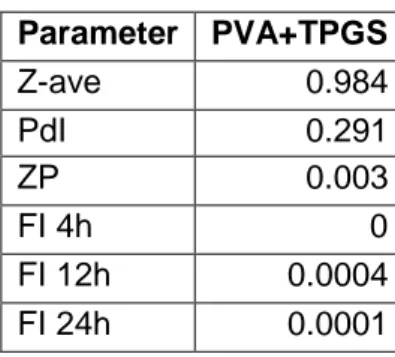
Tables 4 and 5 evaluate whether there are statistically significant differences for each of the 6 parameters (Z-ave, PdI, ZP, FI 4h, FI 12h and FI 24h). In table 4, it is possible to understand that the type of polymer was non-significant to the Z-Ave and PdI parameters. Otherwise, the ZP, the FI at 4 h, 12 h and 24 h were significant for the type of polymer used (PVA + TPGS). This indicates that these measurements showed real differences between the polymer used.
Table 4.ANOVA for the type of polymer (p-values)
Parameter PVA+TPGS Z-ave 0.984 PdI 0.291 ZP 0.003 FI 4h 0 FI 12h 0.0004 FI 24h 0.0001
Table 5 demonstrates that only in the cases of FI at 12 h for the polymer TPGS and FI at 24 h for the polymer PVA the mannose content was significant. This shows that these measurements showed real differences. The mannose content was non-significant to almost all parameters (Z-ave, PdI, ZP and FI).
Table 5. ANOVA for the mannose content (p-values)
Parameters PVA+TPGS PVA TPGS
Z-ave 0.199 0.831 0.118 PdI 0.554 0.185 0.368 ZP 0.923 0.806 0.991 FI 4h 0.715 0.279 0.076 FI 12h 0.585 0.102 0.039 FI 24h 0.733 0.028 0.268 5.3.2. PCA modelling
A PCA model was built with auto-scaled data considering the mentioned properties. A two component model was found to be the most adequate according to the cross-validation method. In figure 13 is possible to see black dots that correspond to the variables included in the model (the loadings), green dots correspond to PVA-mannose formulations and red dots correspond to TPGS-PVA-mannose formulations (the scores). The first principal component (PC) (horizontal) of the analysis separated the NPs with PVA and TPGS, showing that these NPs have significant differences. The
21
second component (vertical) is related essentially with the amount of mannose. Variables relevant to the first component are ZP and FI and to the second components are Z-Ave and PdI. The fluorescence intensity at 4 h, 12 h and 24 h have a high correlation. Otherwise, ZP, Z-Ave and PdI are not highly correlated. The zeta potential is opposite to FI, that is the lower FI the higher ZP approximately. The Z-Ave is opposite to PdI, that is the higher Z-Ave the lower PdI. Variables are like magnets that attract the experience (PdI and TPGS). Mannose primarily influenced size and PdI of NPs. The formulations with PVA-Man 10% and TPGS-Man 10% were the most relevant, while the PVA-Man 40%, PVA-Man 20% and TPGS-Man 0% were the smallest. The higher value of the PdI was obtained for the NPs with PVA-Man 40% and TPGS-Man 0%, whilst the TPGS-Man 10% had the lower PdI. The cells treated with TPGS NPs show higher fluorescence, therefore the cells treated with TPGS-Man 20% are the most fluorescent of all the formulations. The cells treated with PVA NPs reveal fluorescence, but smaller than those with TPGS NPs. The cells treated with PVA-Man 40% are the most fluorescent of all preparations and the cells treated with PVA-Man 0% and PVA-Man 10% ere the less fluorescent.
Figure 13. Results of principal component analysis of fluorescence intensity (FI), polydispersity index (PdI), average size (Z-Ave), zeta potential (ZP), PVA-Mannose 0, 10, 20, 40% and TPGS-Mannose 0,10, 20, 40%
In figure 14 it is possible to verify that blue bars indicate the importance of each variable in the first principal component and the yellow ones indicate the importance of
🀫 PVA-NPs
each variable in the second component (the loadings). FI and ZP are more important in the first PC, instead the average size is more important in the second principal component. PdI was important both the first and second principal components, however in the second was more pronounced. ZP is very negative and FI is very positive and equal between them due to TPGS. Z-Ave and PdI indicate the distribution of the percentage of mannose and there was no linear progression of the amount of mannose. The particles with 10% mannose were the ones with higher size and the lowest are PVA-Man 40% and TPGS-Man 0%. As it was increased the amount of mannose, the size of PVA NPs decreased. Otherwise, the size of TPGS NPs increased with the amount of mannose. This can be also confirmed in figure 13. From a statistical point of view, the amount of mannose was not correlated with the characteristics that were being measured. It is more relevant in particle size but was not statistically significant.
Figure 14. PCA model loadings for the first two principal components: average size (Z-Ave), polydispersity index (PdI), zeta potential (ZP) and fluorescence intensity (FI) at 4h, 12h and 24h.
5.3.3. Prediction
Independent MLR models were developed for the six evaluated parameters. Table 6 represents some figures-of-merit of these models. The cross-validation
🀫 Principal component 1
23
coefficient of determination estimates the quality of the models adjustment ability. The
Z-Ave and FI have cross-validation coefficient determination (R2
CV) closest to one, so
indicating good predictive models.
Table 6. Summary of the MLR models for the six evaluated parameters.
R2
CAL R2CV Q2Y RMSEC RMSECV
Parameters Z-Ave (nm) 0.002 0.88 -1.32 2.99 4.57 PdI 0.34 0.039 -1.49 0.012 0.024 ZP (mV) 0.81 0.59 0.54 0.22 0.33 FI 4 h 0.98 0.92 0.92 2300.59 4058.64 FI 12 h 0.92 0.80 0.79 12605.72 20800.99 FI 24 h 0.93 0.82 0.81 26808.55 43389.05
The RMSEP for the average size parameter is much higher for the TPGS-Man 20% and 40%. In other words, the model tends to overestimate. The model of PVA-Man 20% and 40% represents values of RMSEP inferior and of the same order of magnitude as the RMSEC. Therefore, the model is not overfitted. All models built from the tested formulations have values of RMSEP higher than the RMSEC. This is an indication of some tendency to overfit, especially for the PdI and the zeta potential. The RMSEP for the FI is much lower for all formulations tested. The parameter of PdI is the one who presents similar RMSEC, RMSECV and RMSEP, that is had better predictive capacity.
Table 7 shows the root mean square error of model prediction. The table shows that RMSEP vary from 1.2 to 255.9. The model for the average size of all PVA-Mannose formulations and TPGS-PVA-Mannose 0% and 10% have high errors.
Table 7. Root mean square of error prediction of model predictions (cross validation)
Parameters Formulations Z-Ave (nm) PdI ZP (mV) FI 4h FI 12h FI 24h PVA-Man 0% 6.0 1.8 52.7 9.5 8.7 242.2 PVA-Man 10% 1.4 19.4 2.5 35.5 22.8 96.7 PVA-Man 20% 2.6 16.1 3.3 160.0 255.9 160.2 PVA-Man 40% 3.4 1.4 9.9 5.4 4.8 47.5 TPGS-Man 0% 1.2 1.8 13.7 4.4 2.5 3.4 TPGS-Man 10% 1.7 6.8 7.1 64.2 10.9 9.9 TPGS-Man 20% 16.7 4.7 6.8 8.3 4.0 3.5 TPGS-Man 40% 23.2 1.2 2.7 15.2 22.2 3.8
Only the PVA-Mannose 10% and 20% PdI did not represent high errors. The surface charge of PVA-Mannose 0% and TPGS-Mannose 0% did not have high errors. PVA-Mannose 0% and 40% had high error of FI at 4 and 12 h. TPGS-Mannose 0% and 20% had high error of FI at 4, 12 and 24 h. TPGS-Mannose 10% and 40% had high error of FI at 24 h.
Table 8 showed the percentage error in the cross validation. Z-Ave and ZP had low values of percentage error, instead PdI and FI that had in some cases high percentage errors. In case of PdI, the formulations PVA-Man 10% and 20% and TPGS-Man 10 and 20% had low percentage error. The formulations PVA-TPGS-Man 0%, 10% and 20% and TPGS-Man 10% of FI had low percentage error. FI at 4 h for the TPGS-Man 20% and 40% also had low percentage error. TPGS-Man 40% had low percentage error ate FI 12 h. FI 24 h for the PVA-Man 40% had low percentage errors.
Table 8. Percentage error of model predictions (cross validation)
Parameters Formulations Z-Ave (nm) PdI ZP (mV) FI 4h FI 12h FI 24h PVA-Man 0% -1% -36% 1% 20% 25% -1% PVA-Man 10% 4% 3% -29% 5% 10% 2% PVA-Man 20% -2% -4% 23% 1% -1% 1% PVA-Man 40% -1% 46% 7% -36% -45% -5% TPGS-Man 0% -4% 35% -5% -44% -88% -67% TPGS-Man 10% 3% -9% 10% 3% 20% 23% TPGS-Man 20% 0% 13% 11% 23% 55% 67% TPGS-Man 40% 0% -51% -27% 13% -10% -60% In table 9 is verified the SECV. Almost all the standard errors obtained are acceptable since errors above 2 or below -2 are not acceptable. Only the standard error of fluorescence intensity at 12h of TPGS-Man 0% is closely to that interval, so this can be considered not acceptable.
Table 9.Standard error of model predictions (cross validation)
Parameters Formulations Z-Ave (nm) PdI ZP (mV) FI 4h FI 12h FI 24h PVA-Man 0% -0.3 -1.1 -0.1 0.9 0.7 0.1 PVA-Man 10% 1.5 0.1 1.5 0.3 0.3 0.2 PVA-Man 20% -0.7 -0.1 -1.3 0.1 0.1 0.1
25
TPGS-Man 0% -1.6 1.1 0.2 -1.7 -1.9 -1.4
TPGS-Man 10% 1.2 -0.3 -0.6 0.2 0.5 0.7
TPGS-Man 20% 0.2 0.4 -0.7 1.0 1.3 1.7
TPGS-Man 40% 0.2 -1.5 1.4 0.6 -0.1 -1.3
Table 10 shows that Z-Ave, PdI and FI are in the direction of TPGS, otherwise only ZP is in the direction of PVA. The most important coefficient in mannose is Z-Ave, that have a negative value. This confirms what is possible to see in figures 13 and 14. Table 10. Regression coefficients for the developed MLR models.
Z-Ave PdI ZP FI 4h FI 12h FI 24h PVA/TPGS -0.008 -0.43 0.89 -0.98 -0.95 -0.96 Mannose -0.041 0.40 0.10 0.16 0.16 0.03
The amount of mannose is relevant for the prediction of average size. PVA or TPGS are relevant for the prediction of PdI, surface charge and fluorescence intensity as shown in table 11.
Table 11. Selectivity
Parameters Z-Ave PdI ZP FI 4h FI 12h FI 24h
PVA 0.04 1.2 76.1 37.6 33.02 502.6
TPGS 0.04 1.2 76.1 37.6 33.02 502.6
Mannose 23.4 0.9 0.01 0.03 0.03 0.00099
6. Conclusion
In the present study, the PVA and TPGS polymeric NPs were successfully prepared using continuous homogenization and ultrasonication techniques. Successful functionalization process with targeting ligands exposed at NPs surface and available for receptor binding. The amount of mannose used in the formulation did not induce any alteration in these parameters. The internalization of NPs prepared with TPGS was faster than NPs prepared with PVA, which increased with the addition of mannose (until 20% PLGA-Mannose). The type of polymer was non-significant in terms of the Z-Ave and PdI. The ZP, the FI at 4h, 12h and 24h are significant for the type of polymer used (PVA/TPGS). The mannose content was non-significant for almost all parameters (Z-ave, PdI, ZP and FI). Prediction models were satisfactory (statistically significant for significance 0.05) for NPs size.
Poor predictions were obtained for PdI and ZP meaning that factors influencing these properties were not considered in these models. Predictions for the FI were also inadequate and require more data. A design-space could not be established as the prediction quality did not allow a reliable definition of the design-space. In this sense, more experiments and possibly non-linear models are required.
7. References
1 Fernald, K., and Kurokawa, M. Evading apoptosis in cancer. Trends Cell Biol. 23.
2013. 620–633.doi: 10.1016/j.tcb.2013.07.006
2 Zitvogel, L., Tesniere, A., and Kroemer, G. Cancer despite immune surveillance:
immunoselection and immune subversion. Nat. Rev. Immunol. 6. 2006. 715–727. doi:10.1038/nri1936
3 Lange, J., Lingappa, V., Ganong, W., McPhee, S., Pathophysiology of Disease – An
Introduction to Clinical Medicine; 2ndedition; Lange Medical Book; 1997; 78-98
4 Wu, D., Gao, Y., Qi, Y., Chen, L., Ma, Y., and Li, Y. Peptide-based cancer therapy:
opportunity and challenge. Cancer Lett. 351. 2014. 13–22.doi:10.1016/j. canlet.2014.05.002
5 Peer, D., Karp, J.M., Hong, S., Farokhzad, O.C., Margalit, R., and Langer, R. Nano
carriers as an emerging platform for cancer therapy. Nat. Nanotechnol. 2. 2007. 751– 760. doi:10.1038/nnano.2007.387
6 Helmy, K.Y., Patel, S.A., Nahas, G.R., and Rameshwar, P. Cancer immunotherapy:
accomplishments to date and future promise. Ther. Deliv. 4. 2013. 1307–1320. doi:10.4155/tde.13.88
7 Xu, Z., Wang, Y., Zhang, L., and Huang, L. Nanoparticle delivered transforming
growth factor beta siRNA enhances vaccination against advanced melanoma by modifying tumor microenvironment. ACS Nano 8. 2014. 3636–3645. doi: 10.1021/nn500216y
8 J. Begley, A. Ribas, Targeted therapies to improve tumor immunotherapy, Clin.
Cancer Res. 14 (14). 2008. 4385–4391.
9 P.M. Dimberu, R.M. Leonhardt, Cancer immunotherapy takes a multi-faceted
approach to kick the immune systeminto gear, Yale J. Biol.Med. 84 (4). 2011. 371–380.
10 E. Schlosser, M. Mueller, S. Fischer, S. Basta, D.H. Busch, B. Gander, M. Groettrup,
TLR ligands and antigen need to be coencapsulated into the same biodegradable microsphere for the generation of potent cytotoxic T lymphocyte responses, Vaccine 26