DEVELOPMENT AND APPLICATION OF AN AUTOMATIC TOOL FOR THE SELECTION OF CONTROL VARIABLES BASED ON THE SELF- OPTIMIZING CONTROL METHODOLOGY

Vol. 34, No. 03, pp. 851 – 871, July – September, 2017 dx.doi.org/10.1590/0104-6632.20170343s20150445

* To whom correspondence should be addressed

DEVELOPMENT AND APPLICATION OF AN

AUTOMATIC TOOL FOR THE SELECTION OF

CONTROL VARIABLES BASED ON THE

SELF-OPTIMIZING CONTROL METHODOLOGY

S. K. Silva

_{, S. B. Villar}

_{, A. B. da Costa}

_,

H. C. G. Teixeira

_{and A. C. B. Araújo}

_*

1_{Department of Chemical Engineering, Federal University of Campina Grande} Av. Aprigio Veloso, 882, Campina Grande, PB, Brazil.

*E-mail: antonio.brandao@ufcg.edu.br; Tel: +55 83 21011115

2_{Gerência de Automação e Otimização de Processos, Engenharia Básica, Cenpes/Petrobras} Av. Jequitibá, 950, Cidade Universitária, Ilha do Fundão, Rio de Janeiro, RJ, Brazil.

(Submitted: July 13, 2015; Revised: March 2, 2016; Accepted: March 2, 2016)

Abstract – Rules for control structure design for industrial processes have been extensively proposed in the literature. Some model-based methodologies have a sound mathematical basis, such as the self-optimizing control technology. The procedure can be applied with the aid of available commercial simulators, e.g., PRO/IITM _{and AspenPlus®, from} which the converging results are obtained more suitably for industrial applications, lessening the effort needed to build

an appropriate mathematical model of the plant. Motivated by this context, this work explores the development and application of a tool designed to automatically generate near-optimal controlled structures for process plants based on the self-optimizing control technology. The goal is to provide a means to facilitate the way possible arrangements of

controlled variables are generated. Using the local minimum singular value rule supported by a modified version of a branch-and-bound algorithm, the best sets of candidate controlled variables can be identified that minimize the loss

between real optimal operation and operation under constant set-point policy. A case study consisting of a deethanizer is considered to show the main features of the proposed tool. The conclusion indicates the feasibility of merging complex theoretical contents within the framework of a user-friendly interface simple enough to generate control structures suitable for real world implementation.

Keywords: Control structure design; VBA; PRO/II; Akima and bicubic spline; Minimum singular value; Branch-and-bound.

INTRODUCTION

Optimal operation of process plants is at the foremost front in process engineering applications, but still represents a challenge for plant engineers. This in part is

due to the fact that there are many different methods that

claim to guarantee optimality, and choosing one that best

suits a particular application is sometimes difficult. In addition, there can be many different ways to implement a

given procedure, ranging from plain manual computations to calculations based on several pieces of software from which the user needs to navigate from one to the other, back and forth, just to get the tedious calculations done.

One such promising method to accomplish (near)

of Chemical

optimal operation of process plants is the self-optimizing control technology (Skogestad, 2004). Self-optimizing control is when an acceptable (economic) loss can be achieved using constant set points for the controlled variables, without the need to reoptimize when disturbances occur (Skogestad, 2000). The constant set point policy is simple but will not be optimal (and thus have a positive loss) as a result of the following two factors: (1) disturbances, i.e., changes in (independent) variables and parameters that cause the optimal set points to change, and

(2) implementation errors, i.e., differences between the

setpoints and the actual values of the controlled variables (e.g., because of measurement errors or poor control).

The effect of these factors (or more specifically the loss)

depends on the choice of controlled variables, and the

objective is to find a set of controlled variables for which

the loss is acceptable. Some contributions to the theory of self-optimizing control have been slowly but steadily incorporated into the current state of the technology. Halvorsen et al. (2003) found one way to determine the optimal linear combination of measurements to use as controlled variables, and also derived the approximate singular value rule, which is very useful for quick screening and elimination of poor candidate variables. Hori et al. (2005) considered the case of “perfect indirect control” where one attempts to control a combination of

the available measurements such that there is no effect of

disturbances on the primary outputs at steady-state. Alstad and Skogestad (2007) introduced the null space method for selecting linear combinations of controlled variables, where the objective was to derive a simple method for selecting the optimal measurement combination matrix H for the special case with no implementation error, focusing on minimizing the loss caused by disturbances. Alstad et al. (2009) further improved the null space method, providing an explicit expression for H for the case where the objective is to minimize the combined loss for disturbances and measurement errors, and extending the null space method to cases with extra measurements by using the extra degrees of freedom to minimize the loss caused by measurement errors. This reduced even more the loss caused by keeping these new controlled variables at constant setpoint. Jacobsen and Skogestad (2011) devised a way to determine regions where the active constraints may switch during operation. Jaschke and

Skogestad (2012) presented a method for finding optimal

controlled variables, which are polynomial combinations of measurements, and they claimed that controlling these variables gives optimal steady-state operation. Indeed, that

article contains the first contribution to extend the ideas

of self-optimizing control to the more general class of polynomial systems. However, these ideas, though very promising in the sense of reducing even further the loss in the constant setpoint policy by considering nonlinearities in the system in the form of polynomials, are not considered

in this work. More recently, Graciano et al. (2015) argued that the self-optimizing control is complementary to real time optimization (RTO), and developed a new model predictive control (MPC) strategy with zone control and self-optimizing control variable targets in order to cope with infrequent setpoint updates computed by the RTO. Their results showed that the proposed approach improves the coordination between the RTO and MPC layers and, by giving better performance in between RTO executions, it

also led to a higher overall profit.

Many authors have reported results of the use of the

self-optimizing control technology that ensure the efficiency of

the method applied to a great variety of test-bed examples (e.g., Jensen and Skogestad, 2007a; Jensen and Skogestad, 2007b; Hori and Skogestad, 2007a,b; Lersbamrungsuk et al., 2008; Jagtap et al., 2011; Panahi and Skogestad, 2012; Gera et al., 2013; Jaschke and Skogestad, 2014; Khanam et al., 2014; Graciano et al., 2015). Moreover, application

of this technology to different case studies using process

simulators has also been reported in the literature (Araujo and Skogestad, 2007a; Araujo and Skogestad, 2007b; Baldea, Araujo, and Skogestad, 2008; Araujo and Skogestad, 2008; Araujo and Shang, 2009a; Araujo and Shang, 2009b; Araujo and Shang, 2009c), and the results showed the feasibility and ease of implementation of the self-optimizing control procedure in such instances.

However, much effort and time is usually expended doing many mathematical computations using different pieces

of software quite alike from one another. In general, packages of data collected from the various simulations of the process are exported to some linear algebra software platform, like MatLab®, for calculations involving, e.g., matrix manipulations for building linear approximation models of the nonlinear plant, matrix decompositions for computation of gains, or integer optimizations using branch-and-bound techniques for feature subset selection. Analysis follows the calculation procedures by taking the results to some spreadsheet software like Microsoft® Excel

where reports and plots are generated for final checking

and presentation.

Therefore, one source of resistance to widespread industrial application of mathematically based plantwide control methodologies is related to the fact that too much

effort and energy is usually expended by the engineer

doing several computations to generate only a handful of candidate control structures. Many of these steps consist of calculations involving approximations of the actual process as derived from the converging results of nonlinear mathematical models obtained by exhaustive simulation through the use of some commercial simulator. These approximations appear disguised in the form of linear

models that need to be built and further refined so as to reproduce with high degree of fidelity the main aspects

usually the way one may obtain the gain matrix at zero frequency from simulations on a steady-state nonlinear model of the process using a commercial simulator. For each manipulated variable a run of the simulation yields values for the chosen candidate controlled variables that need to be stored for future calculations. This procedure is repeated for each manipulated variable, and depending on the dimension of the problem it may become an extremely tedious and time consuming task to be executed. Moreover, it is not always clear which step size to apply to generate a suitable linear model, unless the user has a deep knowledge of numerical methods to adjust this choice anytime the simulation results are not consistent.

However, even when a linear model of the plant is

finally determined, much computation is still needed to

select sets of candidate control structures. Particularly, several of these computations involve the use of many features of some linear algebra package depending on the plantwide control technique being used. Manipulations of

functions from these packages can be difficult and generally

require good expertise in mathematical methods, which is precisely what discourages most practitioner engineers who prefer not to devote too much time digging in too deep into mathematical thinking. Here is exactly where a well-tuned automatic tool to overcome these hurdles falls into place.

This work aims at describing the development and implementation of an automatic tool to assist the plant engineer to determine suitable control structures based on the technique of self-optimizing control. The end result should facilitate the use of the method, as well as encourage the application of plantwide control studies

on different cases in the process industry. To the authors’

knowledge, no such a product has been reported previously in the academic and industrial literature to date.

OVERVIEW OF THE SELF-OPTIMIZING CONTROL TECHNOLOGY

The self-optimizing control technology for the selection of controlled variables is the method considered in this work. In this section we give an overview of the technology, but do not present an exhaustive review on the subject. For details, please refer to Skogestad (2000, 2004).

The objective is to achieve self-optimizing control

where fixing the primary controlled variables c at constant

setpoints c_s indirectly leads to near-optimal operation. More precisely (Skogestad, 2004): “Self-optimizing control is when one can achieve an acceptable loss with constant setpoint values for the controlled variables without the need to re-optimize when disturbances occur”.

For continuous processes with infrequent grade

changes, a steady-state analysis is usually sufficient

because the economics can be assumed to be determined by the steady-state operation.

It is assumed that the optimal operation of the system

can be quantified in terms of a scalar (usually highly

nonlinear) cost function (performance index) J₀, which is to be minimized with respect to the available degrees of freedom u₀,

0

0 0

min

( ,

, )

u

J x u d

subject to the (usually highly nonlinear) constraints

1

( ,

, )

0;

( ,

, )

0

g x u d

=

g x u d

≤

Here d represents all of the disturbances, including

exogenous changes that affect the system (e.g., a change in

the feed), changes in the model (typically represented by changes in the function g₁), changes in the specifications (constraints), and changes in the parameters (prices) that enter in the cost function and the constraints. x represents the internal variables (states). One way to approach this problem is to evaluate the cost function for the expected set of disturbances and implementation errors using, e.g., techniques of nonlinear numerical optimization. The main steps of this procedure can be as follows (Skogestad, 2000):

1. Definition of the number of degree of freedom.

2. Definition of optimal operation (definition of the cost function and constraints, including the process model). 3. Identification of important disturbances (typically, feed

flow rates, active constraints and input errors).

4. Numerical optimization of the defined mathematical problem as given, e.g., by Equations 1 and 2.

5. Identification of candidate controlled variables.

6. Evaluation of loss for alternative combinations of controlled variables (loss imposed by keeping constant set points when there are disturbances or implementation errors), including feasibility investigation.

7. Final evaluation and selection (including controllability analysis).

In step 3 the important disturbances as well as their magnitude and frequency are determined based on the experience of the process engineer. These are usually related to the economics of the plant due to long term changes caused by plant throughput, changes in product

specification, prices of raw material, utilities and energy, and

equipment constraints. However, short term disturbances can also be considered, such as input errors due to, e.g., imperfect valves, and changes in feed conditions like temperature, composition, and pressure. These are the kind of disturbances we consider in this work.

The optimization in this case is used to determine the best operating conditions for each important disturbance

as per step 3 above, as well as to define the set of active

(1)

constraints used to select controlled variables. Indeed, to achieve optimal operation, the active constraints are

chosen to be controlled. The difficult issue is to decide

which unconstrained variables c to control.

Unconstrained problem: The original independent variables u₀ are divided into the variables u’, used to satisfy the active constraints g’₂ = 0, and the remaining unconstrained variables u. The value of u’ is then a function of the remaining independent variables (u and d). Similarly, the states x are determined by the value of the remaining independent variables. Thus, by solving the model equations (g₁ = 0), and for the active constraints (g’₂ = 0), one may formally write x = x(u,d) and u’ = u’(u,d), and the cost as a function of u and d becomes J = J₀(x,u₀,d) = J₀(x(u,d), u’(u,d), u, d) = J(u,d).

The remaining unconstrained problem in reduced space

is then given by

min ( , )

u

J x d

where u represents the set of remaining unconstrained degrees of freedom. This unconstrained problem is the basis for the local method introduced below.

Degrees of freedom analysis

It is very important to determine the number of steady-state degrees of freedom because this in turn determines the number of steady-state controlled variables that need to

be chosen. To find them for complex plants, it is useful to

sum the number of degrees for individual units as given in Table 1 (Skogestad, 2002).

Table 1 - Typical number of steady-state degrees of freedom for main process units.

Process unit DOF

Each external feed stream 1 (feedrate)

Splitter n - 1 split fractions (n is the number of exit streams)

Mixer 0

Compressor, turbine, and pump 1 (work)

Adiabatic flash tank 0a

Liquid phase reactor 1 (holdup)

Gas phase reactor 0a

Heat exchanger 1 (duty or net area)

Columns (e.g., distillation) excluding heat exchangers 0(a) _{+ number of side streams}

(a) Add 1 degree of freedom for each extra pressure that is set (need an extra valve, compressor, or pump), e.g., in the flash tank, gas phase reactor, or column.

Local (linear) method

In terms of the unconstrained variables, the loss function around the optimum can be expanded as (Skogestad, 2000):

2 2

1

( , )

( )

2

opt

L

=

J u d

−

J

d

=

z

With:

1/ 2 1/ 2 1

(

)

(

)

uu opt uu opt

z

=

J

u u

−

=

J G

c c

−

where G is the steady-state gain matrix from the unconstrained degrees of freedom u to the controlled variables c (yet to be selected) and J_uu is the Hessian of the cost function with respect to the manipulated variables u. Truly optimal operation corresponds to L = 0, but in general L > 0. A small value of the loss function L is desired as it implies that the plant is operating close to its

optimum. Note that the main issue here is not to find the

optimal set points, but rather to find the right variables to

keep constant.

Assuming that each controlled variable c_i is scaled such that:

' ' '

2

1

c opt

e

=

c

−

c

≤

the worst case loss is given by (Halvorsen, Skogestad, Morud, & Alstad, 2003):

(

)

2

max ₁ 2

1/ 2 1

1

1

max

2

c e

uu

L

L

S GJ

σ

≤ −

=

=









where S₁ is the scaling matrix for c_i given by:

1

1

( )

S

diag

span c





=

_

_





(3)

(4)

(5)

(6)

where span(c_i) = Dc_i,opt(d) + n_i. Here, Dc_i,opt(d) is the variation of c_i due to variation in disturbances and n_i is the implementation error of c_i.

If the matrix J_uu is too cumbersome to be obtained,

and if it is assumed that each ‘‘base variable’’ u has been

scaled such that a unit change in each input has the same

effect on the cost function J (such that the Hessian J_uu is a scalar times a unitary matrix, i.e., J_uu = aU), then Equation 6 becomes

(

)

1

2

L

S G

α

σ

=









where a = s(J_uu). Thus, in order to minimize the loss, L, s(S₁GJ_uu-1/2_{) or alternatively s(S}

1G) should be maximized; the latter is the original minimum singular value rule of Skogestad (2000).

As it can be seen, in the method of selection of self-optimizing control structures we need to obtain the gain matrix G and the Hessian matrix J_uu in order to compute the value of the loss function L. In this work, we used the Akima Cubic Spline interpolation method to obtain these matrices. Moreover, the loss function L depends on the subset of candidate controlled variables that maximize the minimum singular value s(S₁GJ_uu-1/2_{) (or s(S}

1G)). In other words, we start with a big gain matrix G’ where all candidates are included, this gives a tall matrix with more rows than columns. But since the calculation of the loss function uses only a subset of these variables corresponding to exactly the number of unconstrained degrees of freedom, one needs to search among all possible square submatrices G to find the one that gives the maximum minimum singular value according to the formulas in Equation 6 or 8. These subsets can be obtained by a feature selection method. In this work we use the branch-and-bound bidirectional algorithm as described in Cao and Kariwala (2008). The technique takes

advantage of the monotonicity property of the minimum singular value to quickly determine the subset of controlled variables that minimizes the loss function.

In the following subsections, we give a brief review of the mathematical concepts used by the proposed automatic tool to select the best sets of self-optimizing control structures.

Computation of the gain and Hessian matrices

The accuracy with which the gain G and Hessian J_uu matrices are obtained is crucial to the success of the application of the self-optimizing local method described in the last section. However, mathematical models in

commercial process simulators do not make analytical first

or second order derivative information available to the user. Therefore, numerical, less precise methods are the only viable manner to derive such information.

G and J_uu are calculated with respect to the nominal optimal operating point, i.e., when disturbances are nominal. One straightforward way to numerically obtain the gain matrix G is to use finite differences, like the simple

first order forward difference approximation in Equation 9,

to compute each element G_i,j (Araujo et al., 2007a).

0

(

)

( )

( )

lim

c u

e h

c u

c u

u

h

+

−

∂

₌

∂

where i = 1, …, n_c is the index set of candidate variables, j = 1, …, n_u is the index set of manipulated variables, h is the vector of increments for each input u_j, and e_j = [0 0 0 … 1 … 0] is the zero vector except for the jth-element which is 1.

The Hessian J_uu can be similarly evaluated by, e.g., the following simple approximation in Equation 10 (Araujo et al., 2007a). 0

(

)

(

)

(

)

( )

( )

lim

[

]

ii jj ii jj

T h

i j ij

J u

E h

E h

J u

E h

J u

E h

J u

J u

u u

hh

+

+

−

+

−

+

+

∂

=

∂ ∂

where E_ij is the zero matrix except for the ij-element which is 1.

Equation 9 has a significant advantage, that is to say,

the realization of a single increment for obtaining the gain element G_i,j. However, one important factor to be addressed is the accuracy of the above computation, since G_i,j is being evaluated at a single point, and it is known that the accuracy increases as higher order methods that compute the value of the function at more points are used. Moreover, the size of the increment is hard to determine due to both rounding error and formula error. These problems become even more serious when the objective is to compute the Hessian

matrix J_uu, a matrix of second derivatives, as shown in Equation 10.

A workaround to achieve better accuracy without the

instability problems common to finite difference methods

is to use polynomial approximations. In this work we use the piecewise cubic polynomial approximation of each G_i,j via the Akima cubic spline, as well as each element of the Hessian matrix J_uu via the bicubic spline. It is important to note that, like any other numerical method used to compute second derivatives, high accuracy in the calculation of the Hessian matrix cannot be guaranteed due to intrinsic sensitivity of the approximation, unless an analytical (8)

(9)

solution can be employed, which does not happen in the majority of the cases. This is why in the present work we used the bicubic spline to compute the Hessian matrix J_uu due to its smoothness property to obtain the best non-linear (polynomial) approximation from simulation data around the desired operating point.

The advantage of employing piecewise cubic spline polynomial functions of higher degree may be seen in certain applications, e.g., when a smooth function

undergoes an abrupt change somewhere in the region of interest, in which case the approximation gets very unstable and inaccurate, as it happens with, e.g., the natural spline approximation since it utilizes all data points

simultaneously to calculate the coefficients for the entire

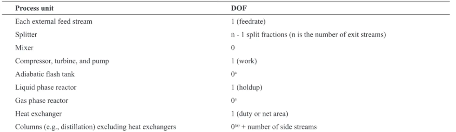
range of interpolation. As a consequence, one may expect possible oscillations in the vicinity of a point outside the curve, as shown in Figure 1.

Figure 1. Behavior of the natural spline vis-à-vis the Akima spline showing oscillation of the former around an outlier

Thus, one disadvantage of cubic splines is that they could oscillate in the neighbourhood of an outlier. On the graph of Figure 1 one can see a set of points having one outlier. The cubic spline with boundary conditions is green-coloured. On the intervals which are next to the outlier, the spline noticeably deviates from the given function because of the outlier. The Akima spline is red-coloured. It can be seen that, in contrast to the cubic spline, the Akima spline

is less affected by the outliers. In other words, the Akima

spline is a special spline which is stable to the outliers, and this is one of the reasons this spline interpolation technique was used in this work to avoid these oscillations which can seriously compromise the computation of the elements of the gain matrix G, which is very sensitive to such degenerations.

The method of Akima (1969) is based on a piecewise function given by a polynomial of the third order in each interval for the case of a single-valued function. In this case the method is somewhat similar to the natural spline function of degree three. As in the spline function,

the continuity of the function itself and of its first-order

derivative is assumed. However, instead of assuming the continuity of the second-order derivative as in the third-order spline function, the Akima method determines the direction of the tangent locally under certain assumptions. By doing so, a curve piecewise to the given set of data

points can be fitted without having discontinuities in the

curve and its slope, and this represents an advantage of the Akima spline over the other spline interpolation methods, which improves the accuracy of the interpolation. This is yet another reason to use this interpolation method in this work since data points between interpolation points can be predicted more accurately, and as a result derivatives can be calculated more precisely to determine the gain matrix G.

It is assumed that the direction of the slope of the curve at a given point (x_i, x_i+1) is determined by the coordinates

of five points f_i-2, f_i-1, f_i, f_i+1, and f_i+2, the function values in the vicinity of the point in question. In other words, points that are more than two intervals away are assumed not to

affect the determination of the slope. The coefficients of

the piecewise cubic polynomial are adjusted locally, which in turn requires information only about the points in the vicinity of the range of interpolation. In other words, the function values at (x_i, x_i+1) depend on the values of f_i-2, f_i-1, f_i, f_i+1, and f_i+2. The idea of the method is to obtain the slope of the curve at each point, thus ensuring the continuity of the

first and second derivatives. The method then assumes that the slope of the curve is given by five points, i.e., the point

of interest being the centre point, two points downstream and two upstream (Akima, 1969; Dubey and Upadhyay,

5) in coordinate plane, the slope of the curve at the central point is given by Equation 11:

(

)

(

)

m m m m m m

t

m m m m

− + −

=

− + −

where m₁, m₂, m₃ e m₄ are the slopes of the lines given by the segments 45, 34, 23, and 12, respectively.

The slope of the curve at point 3 depends only on the slopes of four segments, regardless of the interval between them. When m₁ = m₂and m₃ = m₄, Equation 11 returns a

different result for t. In this case, t is recalculated using an arithmetic average of the values of m₂and m₃, i.e.:

(

)

2

m m

t= +

When the slopes of the curves for the set of points are obtained, four boundary conditions are used to determine the piecewise polynomial, namely:

1

and

at

dy

y

y

t

x

x

dx

=

=

=

2

and

at

dy

y

y

t

x

x

dx

=

=

=

where y is the piecewise cubic polynomial:

(

)

(

)

(

)

0 1 1 2 1 3 1

y=p +p x−x +p x−x +p x−x

The coefficients p₀, p₁, p₂ and p₃ are determined by applying the boundary conditions in Equations 13 and 14 to Equation 15. This produces the following expressions

for the coefficients:

0 1

p =y

1 1 p =t

(

)

(

)

(

)

(

)

(

)

(

)

2 y y

t t x x p x x  −  + −  ₋    = −

Note that the interpolated points are independent of the scaling of the x and y axes. After obtaining the

piecewise cubic polynomials in each interval, first and

second order derivatives are then calculated by analytically

differentiating Equation 15 with respect to x, therefore

producing the gain matrix.

In order to reflect the true nature of the Akima method when applied to smooth curve fitting some aspects must

be considered. Since the method interpolates the given data points it is applicable only to the case where the precise values of the coordinates of the points are given. It should be recognized that all experimental data have some errors in them, and unless the errors are negligible it

is more appropriate to smooth the data, i.e., to fit a curve approximating the data appropriately, than to fit a curve

passing through all the points. In the present work our set of points is deterministically calculated by a commercial simulator, therefore no error is attributed due to experiment. Use of this method is not recommended when given data points manifest apparent regularity or when we have a priori knowledge on the regularity of the data. This is not the case when working with information obtained from simulations using a mathematical model since no one can guarantee regularity of the data. As is true for any method of interpolation, no assurance can be given of the accuracy of the interpolation, unless the method in question has been checked in advance against precise values or a functional form. The method yields a smooth and natural curve and is therefore useful in cases where manual, but tedious, curve

fitting will do in principle. This is clearly the reason why it

is used in situations like the one approached in this work. For single-valued functions, the resultant curve is invariant under a linear-scale transformation of the coordinate

system. In other words, different scalings of the coordinates

result in the same curve. This favors the use of scaling of the manipulated and specially controlled variables that otherwise can vary widely in magnitude.

In the computation of J_uu we seek an estimate of J(u₁, u₂, …, u_nu) from an n-dimensional grid of tabulated values of J and n one-dimensional vectors giving the tabulated values of each of the independent variables u₁, u₂, …, u_nu. In two dimensions (the case of more dimensions being analogous in every way), suppose a matrix with function

values J’[1…m][1…n] is available as obtained, e.g., from

simulations in a commercial simulator. The values of each element of the vectors u₁’[1…m] and u₂’[1…n] are also

given. Then we have that J’[j][k] = J(u1’[j], u2’[k]), and we

desire to estimate, by interpolation, the function J at some not tabulated point (u₁, u₂). In a square grid this would correspond to having u₁’[j] £ u₁ £ u₁’[j+1] and u₂’[k] £ u₂

£ u2’[k+1] such that J1 º J’[j][k], J2 º J’[j+1][k], J3 º J’[j+1]

4 4

1 1 1 2

1 1

( ,

)

i j

J u u

c t v

= =

=

∑∑

( ,

)

(

1)

i j

J u u

dt

i

c t

v

u

du





∂

=

−

_

_

∂

∑∑

_

_

( ,

)

(

1)

i j

J u u

dv

j

c t v

u

du





∂

₌

₋





∂

∑∑

_

_

2 4 4

2 2

1 2

1 1

1 2 1 2

( ,

)

(

1)(

1)

i j

J u u

dt

dv

i

j

c t

v

u u

du

du

− − = =







∂

₌

₋

₋







∂ ∂

∑∑

_

_

_

where the scaled coordinates t and v are given, e.g., by Equations 21 and 22, respectively.

1 1

1 1

'[ ]

'[

1]

'[ ]

u

u

j

t

u

j

u

j



−



≡ 

_{+ −}







'[ ]

'[

1]

'[ ]

u

u

k

v

u

k

u

k



−



≡ 

_{+ −}







The quantities c_ij are obtained from the functions and derivative values are a complicated linear transformation,

with coefficients which, having been determined once

in the mists of numerical history, can be tabulated and forgotten. In order to increase smoothness, the values of the derivatives at the grid points are determined globally by one-dimensional splines. To interpolate one functional value, m one-dimensional splines across the row of the table are performed, followed by one additional one-dimensional spline down the newly created column. However, to save precomputation and storage of all derivative information, spline users typically precompute and store only one auxiliary table of secondary derivatives in one direction only, then one need only do spline evaluations (not constructions) for the m row splines. Nevertheless, a

construction and evaluation is still necessary for the final

column spline. For more information on this procedure, the reader is referred to Numerical Recipes (2007). After numerically obtaining the Hessian matrix J_uu, we still need

to do a slight adjustment to make it positive definite. To this end we perform a modified Cholesky factorization

(Nocedal and Wright, 2006), which guarantees that the

final Hessian is positive definite without modifying it

substantially. This is done by increasing the diagonal elements of J_uu encountered during the factorization (where

necessary) to ensure they are sufficiently positive.

The branch-and-bound method for variable selection

In the self-optimizing control technology, the number of candidate controlled variables should naturally exceed the number of unconstrained degrees of freedom for the

definition of the control structure (Skogestad, 2000).

Therefore the gain matrix G’ is usually a tall matrix, and one needs to select those rows (controlled variables) that maximize the minimum singular value of S₁GJ_uu-1/2 _(or S₁G) according to the maximum singular value rule, as discussed previously.

Screening through all possible subsets of controlled variables, i.e., all possible square G matrices, one at time in order to evaluate s(S₁GJ_uu-1/2_{) (or s(S}

1G)) can be

overwhelming even for small problems due to the effect

of the combinatorial explosion. For example, with 10 unconstrained degrees of freedom and 50 candidate controlled variables, which represents a modest process plant, there are:

10

50

50!

1 02722781 10

10

10!40!

.

 

=

=

×

 

 

possible control structures, without including the alternative ways of controlling inventories. Clearly, an analysis of all of them is intractable.

Fortunately, methods of feature selection applied to

variable selection overcome this problem quite effectively.

One such method, and the one used in this work, is the branch-and-bound algorithm. This global optimization technique, also known as branching and pruning, can solve combinatorial problems of selecting subsets of variables without the need for thorough evaluation of all existing

subsets in the problem. Since its first appearance in the

literature as proposed by Lawlere and Wood (1966) and

further modified to introduce a simplified algorithm that

could be used in subroutines (Narendra & Fukunaga, 1977), (20)

(21)

the technique has been improved to make the method still

more efficient, with fewer iterations and runtime (Cao

& Saha, 2005; Cao & Kariwala, 2008; Kariwala & Cao, 2009; Saha & Cao, 2003).

The principle underlying the branch-and-bound algorithm for subset selection is based on the fact that

resolving a difficult problem can be equivalent to solving

a series of simple related problems derived from the main problem such that the solution to these simple problems can lead to the solution of the original problem. If the solution is not adequate, the subdivision of the problem is repeated until there are no more sub-problems to be solved. This is the general principle of the branch-and-bound algorithm.

Suppose X_S = {x₁, x₂, …, x_S} is a set of S elements and suppose a subset X_n with n elements is selected from X_S (X_n ⊂X_S). Thus, there are S!/n!(S – n)! possible ways of selecting X_n subsets out of X_S. If we let Γ be the criterion function used during the selection procedure, then there is a subset of n elements, denoted X*

n, which satisfies the following equality:

( )

( )

max

X

X

Γ

=

Γ

Thus, we can say that X*

n is the global optimal subset solution of Equation 23 with respect to the criterion Γ. It is assumed that the criterion function Γ satisfies the monotonicity property given by:

(

X

)

(

X

), if

X

X

Γ

≤ Γ

⊆

According to this property a subset with fewer variables cannot be better than any larger set containing this subset (Saha & Cao, 2003).

Ordinary branch-and-bound algorithms are unidirectional, in a sense that either the subsets can be shrunk one by one until the target size, or the subsets can be expanded until reaching the desired size. In the case of the descending branch-and-bound algorithm, suppose m >

n and that Γn

( )

subsets of m elements, X_m, i.e.:

( )

( )

n m

n m n

X X

X X

⊆

Γ ≥ Γ

Additionally, let B be the lower limit of Γ(X* n), or:

( )

n

B≤ Γ X

So, it follows that:

( )

( )

( )

if Γn Xm <B, Γ Xn < Γ Xn ∀Xn⊆Xm

Th condition described in Equation 27 indicates that no subset of X_m can be an optimal subset. Thus, X_m and all subsets thereof can be discarded without further evaluation. Analogously, the selection of a subset can also be performed in ascending order. An upward search starting from an empty set gradually expands the superset element by element to achieve the size requirements for a subset. Cao and Kariwala (2003) showed that if we assume B as the lower limit of Γ(X*

n) as defined in Equation 25, and taking Γn( )Xm _{(with m < n) as an upper limit upward on all}

Γ subsets of m elements X_m, it follows that:

( )

( )

n m

n m n

X X

X X

⊇

Γ ≥ Γ

Therefore,

( )

( )

( )

if Γn Xm <B, Γ Xn < Γ Xn ∀Xn⊇Xm

Equation 29 guarantees that none of the supra sets X_m can be globally optimal. Therefore, X_m and their supra sets can be pruned without additional considerations.

In this work, in order to obtain the best sets of controlled variables using the branch-and-bound technique just described we used the bidirectional branch-and-bound algorithm proposed by Cao & Kariwala (2008), where the search is carried out in both directions, making

this a much more efficient method than traditional

unidirectional branch-and-bound algorithms. The code was re-implemented as a Visual Basic for Application (VBA) subroutine based on the original implementation developed by Dr. Yi Cao using Matlab® _{7.4 (R2007a)}

that can be found in the File Exchange on the MathWorks website (the complete code can be found in the MathWorks File Exchange website under the following address: http://

www.mathworks.com/matlabcentral/fileexchange/17480- bidirectional-branch-and-bound-minimum-singular-value-solver-v2, accessed on September 10, 2013).

Monotonicity of the minimum singular value. The criterion function for the branch-and-bound algorithm used in this work is obviously the minimum singular value, and the only limitation to use the method just described is that this criterion function must satisfy the monotonicity property of Equation 24. Suppose G’ is the system’s gain matrix of unconstrained variables u comprising all the candidate controlled variables for the selection. Take a subset of these variables that corresponds to the

selection of a row of G’. Assume [ 1, , ]

T S

g g _{and denote}

1,

T

i i i

G = G− g 

, where i = n,..., S. Then, it can be shown that the monotonicity of the minimum singular value means:

( )

(

)

( )

r Gn r Gn r GS

σ

σ

σ

Therefore, since the minimum singular value possesses the monotonicity property, global optimality is always guaranteed using the branch-and-bound method. For more results on this refer to Cao et al. (1998).

As the selection of manipulated variables is determined by the user, it is prone to generate singular gain matrices, that

is to say, matrices with column rank deficiency. Therefore,

as a matter of precaution, a safeguard check of the rank of G’ obtained by the Akima cubic spline is performed prior to the application of the branch-and-bound technique. If the calculated rank of G’ is found to be deficient then the branch-and-bound technique is applied to select the best sets of manipulated variables. After choosing a suitable set,

the calculations are then resumed to find the best sets of

controlled variables.

DEVELOPMENT OF THE PROPOSED AUTOMATIC TOOL

Studies like the ones reported by Araujo and Skogestad (2007a), Araujo and Skogestad (2007b), Araujo and Skogestad (2008), and in the PhD thesis of Araujo (2007) under the supervision of Dr. Sigurd Skogestad, use mathematical models of whole large scale processes at steady state derived from the commercial simulator Aspen Plus®. From these models, simulations are performed and

the information needed to obtain the gain matrix G’ is read

in Microsoft Excel® with the aid of the OLE technology (Windows® Object Linking and Embedding). However, the evaluation of G’, the calculation of the Hessian matrix, inverse matrix computation, minimum singular values calculations, and branch-and-bound optimization were done using the arsenal of mathematical tools available in Matlab®.

As this work aims at minimizing the effort expended

by the engineer when executing the most laborious steps of the method, such as construction of the gain matrix and obtaining the best sets of variables, we then chose Microsoft Excel® as the platform for user interaction integrated with the commercial simulator PRO/IITM ₍₂₀₁₂₎

for model simulation. These choices were dictated by the widespread and easy use of Microsoft Excel® (here we

used Microsoft Office 2010) with its known Visual Basic®

Editor (VBE) where applications with Visual Basic® _for

Applications (VBA) can be developed. Moreover, the software for process simulation development at steady state, PRO/IITM _{version 9.1, allows for process design and}

operational analysis, which was developed for rigorous calculations of mass and energy balances for a wide range

of chemical, petrochemical, and refining processes. The

choice of PRO/IITM _{was due to stable communication}

with Microsoft Excel® via COM technology (described in more detail in the next section), in addition to detailed documentation giving step-by-step instructions on how to

efficiently transfer data between both platforms (Invensys,

2011).

Communicating Microsoft Excel® with PRO/IITM

Microsoft Excel® _{and PRO/II}TM _{communicate via}

Component Object Model (COM) technology under Microsoft Windows®_{. The PRO/II}TM _{architecture for}

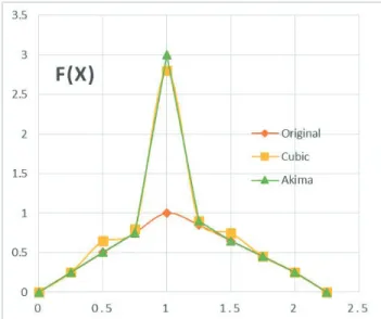
communication using COM technology is better visualized in Figure 2.

According to the Invensys’s COM Server Programmer’s

Guides and Tutorial (Invensys, 2008), the COM server consists of the following parts:

● The PRO/IITM _{COM server provides support for COM}

interface on PRO/IITM_{. Other applications written in}

Microsoft Excel®, Visual Basic, C++, and any other language with COM communication interacts with this interface.

● The PRO/IITM server’s consists of several DLLs

(Dynamic Link Library). This includes functions that access and manage data objects from PRO/IITM _{such as}

routines that calculate properties of a process stream.

● The PRO/IITM _{Database (with extension .prz) contains}

all the data need to model and run the simulation.

Users with access to the PRO/IITM _{COM server include}

applications in VB, Excel Macro, C++, C #, Java, Matlab or any other application that supports COM technology. In this work, the application uses subroutines built in the Visual Basic for Application in Microsoft Excel®_.

The PRO/IITM _{Database is the place where all data}

objects are stored. To access this information, the class of

the object and its respective attribute need to be identified.

For example, the class can be of type “Stream”, which

identifies the creation of a stream object and the reading

of, e.g. the “temperature” attribute of this stream results in

the record of the temperature of the specified stream. All

classes and attributes of a given simulation can be easily

found in the Invensys’s COM Server Reference Guide

(Invensys, 2011).

In order to establish an efficient communication between

Microsoft Excel® _{and PRO/II}TM_{, several subroutines}

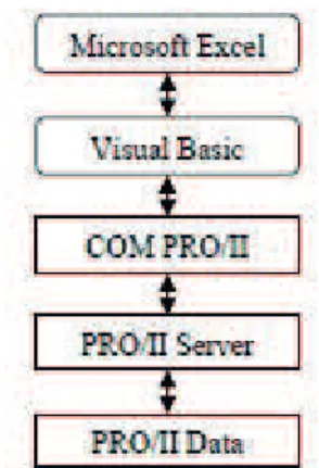
needed to be created within VBA abiding to the logic and structure of the two pieces of software to provide the main commands used to create, access, read, write and close objects. Access to variables in such architecture and the way their values are retrieved is showed in Figure 3 where the basic required operations are also depicted.

Figure 3. Flow configuration using COM technology.

The required syntax to determine the connection between Microsoft Excel® _{and PRO/II can be found in the} manuals COM Server Programmer’s Guides and Tutorial

and COM Server Reference Guide (Invensys, 2011).

Implementation of the automatic tool

In Figure 4 we show the flow diagram of the main

operations performed automatically to determined best sets of controlled variables using the proposed automatic tool.

Once the set of manipulated variables (u_i) (each disturbances d_i is chosen among the set of manipulated variables), and the set of candidate controlled variables (c_i)

are defined by the user via the Graphical User Interface

(GUI), the gain matrix G’ and the Hessian matrix J_uu can be computed (in this version of the proposed automatic tool, G’ is computed with respect to the vector of manipulated variables). The left part of Figure 4 describes how J_uu is computed, while the right part describes how G’ is computed. For each u_j selected (j = 1, …, n_u), the next

u_k’s (k = j, …, n_u) are selected and added to an increment to compute a row in the upper triangular part of J_uu. The resulting vectors containing the values of the vector of candidate controlled variables c for each u_j and the corresponding values of the cost function J_jk are sent to the

subroutine that computes the Akima cubic spline and first

derivatives (G_ij) as well as J_uu. Then the branch-and-bound algorithm is applied to the singular value of the scaled problem using this information, and the resulting best 20 sets of controlled variables are printed on the screen.

How numerically accurate G’ and J_uu are obtained depends on how many points are used for interpolation; the more points available the more accurate they will be. However, too many points will increase substantially the

computation time since for each point one pass of the flow

diagram of Figure 3 is required, because that is the way PRO/IITM _{communicates with Microsoft Excel}®_{. Therefore,} it is convenient to fix the maximum number of points.

The process model in PRO/II is simulated several times

in the inner loop to generate points to define the gain matrix

G’. The resulting grid point is then processed by the Akima cubic routine used to generate the spline for each candidate controlled variable c_i as a function of each manipulated variable u_i. We here make use of the freely available package Alglib® _{(Alglib, 2013) to conduct all the algebraic}

computations to this end. Alglib® _{has a large set of numerical}

programming routines in, e.g., linear algebra, optimization,

and differentiation methods, written in VB, VB.Net, C#, C++ and cPhyton that efficiently performs all the necessary

calculations. The splines in this work are generated using the Alglib® _{functions: spline1dbuildakima(u}

j , cj, t, k),

spline1ddiff(k, p, s, ds, d2s), spline2dbuildbicubic (u, u, J, M, N, C), spline2ddiff(C, ui, uj, J, Jui, Juj, Juiuj).

In the branch-and-bound block of the diagram of

Figure 4, we first determine whether the rank of G’ is full, as discussed above. Otherwise, the best reduced set of manipulated variables with full rank is chosen. Here the tool also has the option to let the user decide upon a suitable set of manipulated variables that best suits a

particular application. After defining the ultimate gain

matrix G’, the branch-and-bound procedure is applied for the selection of best subsets of controlled variables based on the maximization of the minimum singular, as also described above.

Graphical Interface and Handling

As mentioned previously, the objective of the proposed automatic tool is to facilitate the appropriate selection of

the best sets of controlled variables without much effort by the user. For this purpose, an efficient and easy-to-use

Figure 4. Flow diagram of main steps performed by the automatic tool.

The following bullets describe the main functionalities of the graphical interface of Figure 5:

1. Configuration tab.

2. Displays the name of the selected PRO/II (.prz

extension) file.

3. Button used to load all the configured variables from the PRO/II model for selection using the graphical

windows labeled Disturbance, Input Variables, and Output Variables.

4. Options for selecting the method for calculating the gain matrix.

5. Activation of the calculation of the Hessian matrix of the cost function. In this case, it is mandatory to insert a cost function in the PRO/II model.

7. Progress bars. The upper progress bar shows the progress of the steps being processed in each of the selected methods in parts 4 and 5 above. The lower bar shows the overall progress.

8. Button used to remove the last variable entered in the worksheet.

9. Opens or closes the PRO/II model interface previously

defined in part 2.

10. Button to cancel the execution of the procedure being performed by the tool.

11. Message log. Displays the procedure being currently carried out by the tool.

12. Button used to exit the tool. It stays disabled during computations.

13. Button to select the PRO/II process model (.prz) file to be worked out by the tool.

14. Button to clean up the worksheet. All data written by the tool in the worksheet labeled “BRPWC” is erased. 15. Tab with the results of the possible sets of manipulated

variables and the best sets of candidate controlled variables. Figure 6 shows in more detail the display lists for the sets of manipulated variables and controlled variables.

After deciding on which independent manipulated variables and disturbance as well as candidate controlled variables are selected, these are written on a worksheet where the user can have an overview of the variable

configuration. Figure 7 shows an instance of a worksheet

with some selected variables.

The element 15 of Figure 5 displays the tab used to show the sets of variables (manipulated and controlled variables) obtained by applying the branch-and-bound technique. Figure 6 shows the main features available in this tab.

16. Command to calculate the best sets of controlled variables.

17. Button used to load available sets of manipulated variables and their respective minimum singular values in descending order as computed by the

branch-and-bound routine in the canvas below (see bullet 18). 18. Displays the results of the minimum singular value for

sets of manipulated variables used in the generation of the gain matrix. Upon selecting any given row, the gain matrix G’ is computed based on the corresponding set of manipulated variables.

19. List of the best sets of controlled variables and their respective minimum singular values in descending

order. The first column shows the minimum singular

value, and in the following columns the indexed set of controlled variables numbered according to their position in the worksheet depicted in Figure 7. For instance, in Figure 6 the highlighted row displays controlled variables 3 and 6, which in Figure 7

correspond to the molar flow rate of stream B and the reflux rate of equipment T1, respectively.

Figur

e 7.

W

20. Button used to load the best sets of controlled variables and their respective minimum singular values in descending order in the canvas (see bullet 19).

21. Command to calculate the RGA matrix for a given set of controlled variable selected in the canvas 19 by the user. This will be displayed in a separate worksheet. 22. Button to exit the tool.

After execution, a worksheet labeled “Report_Spl” stores the results of the computations for analysis. The gain matrix is further split into two parts, one due to manipulated variables and the other due to disturbances. They are written separately in two new worksheets labeled “Gmatrix_Spl” and “Gdmatrix_Spl”, respectively. The sets of controlled variables determined by the method, as well as their respective minimum singular values, are written in the worksheet “SetOfVariables_Slp”.

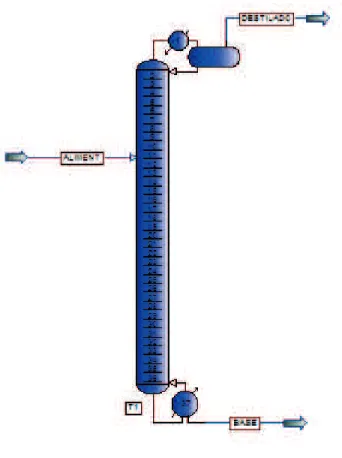
DEETHANIZER COLUMN CASE STUDY

In this section we explore an example application using the proposed automatic tool. The process consists of the separation of ethane from a mixture of propene and propane, and isomers of butane using a distillation column (Hori and Skogestad, 2007a). A schematic of the deethanizer column is shown in Figure 8.

Figure 8. Flowsheet of the deethanizer column.

A feed stream (stream ALIMENT) with average composition described in Table 2 feeds the distillation column where it splits into an overhead vapor distillate (stream DESTILADO) containing basically ethane and some propene, and a bottom product (stream BASE) comprised essentially of propane. The 37 stage column (including reboiler and condenser) operates under a top pressure of 19.2 kg/cm2_{, and is modeled in PRO/II as an}

equilibrium stage column. The thermodynamic model used for modeling was the SRK equation of state and liquid density was calculated by the API method.

Table 2. Feed stream data (stream ALIMENT).

Ethane mole fraction 0.021

Propane mole fraction 0.598

Iso-Butane mole fraction 0.125

n-Butane mole fraction 0.006

Propene mole fraction 0.25

Flow rate (ton/h) 150

Feed stage (from top) 11

Feed temperature (o_{C) 65}

Degrees of freedom

We consider nominal operation with fixed throughput.

Moreover, dynamic degrees of freedom, which include inventories, need to be controlled to ensure stable operation. Therefore, we are left with a certain number of steady-state degrees of freedom, some of which for optimization.

There are a total of 6 dynamic degrees of freedom for the deethanizer column system, which include the

upstream feed flow, which is fixed at the nominal value (see Table 2); two liquid levels, i.e., bottom level and reflux

drum level, that must be controlled for stable operation;

column pressure, which here we consider fixed at the

nominal value; and bottom and top compositions of some key components. Therefore, we are left with 2 steady-state degrees of freedom for optimization.

There are four variables that can be chosen as manipulated variables in the unconstrained case. These are u₀ = [D, V, B, L], where D is the distillate flow rate, V is the boil-up rate, B is the bottom flow rate and L is

the reflux flow rate. This gives 6 possible combinations of

pairs of these manipulated variables. We can also consider nonlinear combinations of these and F, the feed flow rate, e.g. L/D, L/F, V/B, V/F, D/F, and B/F, as is sometimes done in industrial practice. As our objective here in this work is to present the capabilities of the proposed automatic tool and not to investigate the case study thoroughly, we choose the set u = [B, V] as manipulated variables corresponding to the 2 steady-state degrees of freedom. Note that B gives an indirect measure of energy requirements for the column, so it may be an advantage to keep it constant despite disturbances. As disturbances we consider the propane

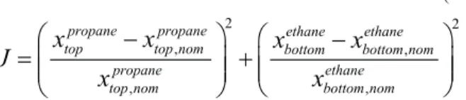
Optimization

The objective is to ensure product specification, and we

here consider deviation from nominal operation as given by the following cost function that needs to be minimized.

2 2

, ,

, ,

propane propane ethane ethane top top nom bottom bottom nom

propane ethane

top nom bottom nom

x

x

x

x

J

x

x



−





−



=



_



_

+



_



_









In Equation 31, x is the component molar fraction and “nom” stands for nominal value, and top and bottom are the DESTILADO and BASE streams, respectively. We constrain

the column operation to guarantee product specification

such that

x

≤

0.15 and

x

≤

0.01

Clearly, optimal operation is achieved when there is no deviation from nominal operation, in which case J = 0 and the two constraints are active. Thus, we would have no degrees of freedom for optimization since the problem is constrained. However, control of composition is known to

be difficult due to measurement delay and sensor reliability.

Therefore, we assume indirect control of composition using more accessible secondary variables such that the deviation as given by Equation 31 is minimized. In other words, we select sets of controlled variables to assure self-optimizing control of the process by applying the minimum singular

value rule. To this end, we will use the proposed automatic tool for computations.

Selection of secondary controlled variables

We here follow Hori and Skogestad (2007a) and choose to select candidate controlled variables that are promptly

measured. These are stage temperatures, flow rates, and flow rates ratios. We chose stages where temperature

change is large, and found that stages 2 (T2), 7 (T7), 10 (T10), 19 (T19), 25 (T25), and 34 (T34) are suitable for temperature measurements. We also consider the temperature of the bottom (TB) and distillate (TD). Bottom (B) and distillate (D) flow rates are included in the set of candidate controlled variables, as well as the following ratios: L/D (reflux ratio, LD), L/F (reflux rate to feed flow rate ratio, LF), V/B (boil-up rate to bottom flow rate ratio, VB), V/F (boil-up rate to feed flow rate ratio, VF), D/F

(distillate flow rate to feed flow rate ratio, DF), and B/F

(bottom flow rate to feed flow rate ratio, BF). We therefore end up with a set of 16 candidates given as c = [T2, T7, T10, T19, T25, T34, TB, TD, B, D, LD, LF, VB, VF, DF, BF].

In Figure 9 the problem set up as configured using the

proposed automatic tool is depicted. Note that calculation of the Hessian matrix, J_uu, is also required. So, we measure the loss as given by s(S₁GJ_uu-1/2_).

Figure 9. Set up interface of the variable selection for the deethanizer case study.

In Table 3, the results obtained after running the automatic tool shows 16 sets of possible pairs of candidate controlled variables sorted by the minimum singular value,

s(S₁GJ_uu-1/2_{). As seen from Table 3, “comfortable” operation} can be achieved by keeping one of the manipulated