Common cycles in macroeconomic aggregates (revised version)

...

.

.

COMMON CYCLES IN MACROECONOMIC AGGREGATES

João Victor

Isslo

Farshid Vahid

(Revised version)

by

João Vil:tor Issler Getulio Vargas Foundation Graduate School of Economics - EPGE

Praia de Botafogo 190 Rio de Janeiro. RJ 22253-900 Brazil and Farshid Vahid Texas A&M Department of Economics College of Liberal Arts College Station. TX 77X43-422X

USA

First draft: September 1'-)'-)3 Revised: August 1994

ABSTRACT

Although there has beell substantial research on long-run co-movement (common trends) in the empirical ma<.:roecollomics literature. little or no work has been done on short run co-movement (col11mon cydes). Investigating common cycles is imponant on two grounds: first. their existence is an impli<.:ation of most dynamic macroeconomic models. Second. they impose imponant restrictions on dynamic systems. whi<.:h <.:an be used for effident estimation and fore<.:asting. In this paper. using a methodology that takes into account short- and long-run co-movement restrictions. we investigate their existence in a multivariate data set <.:ontaining U.S. per-\:apita output. consumption. and investment. As predicted by theory. the data have common trends and common cydes. Based on the results of a post-sample forecasting comparison between restricted and unrestricted dynami<.: systems. we show that a non-trivialloss of effidency results when common qdes are igllored. If pennanent shocks are associated with changes in productivity. the latter fails to be an important source of variation for output and invesnnent contradicting simple aggregate dynamic modcls. Nevertheless. these shocks play a very important role in explaining the variation of consumption. showillg evidence of smoothing. FurthemlOre. it seems that permallellt shocks to output play a much more important role in explaillillg unemployment flu<.:tuations than previously thought.

Acknowledgements: We gratefully ackllowledge comments from Robert F. Ellgle. Pedro

C.

Ferreira. Clive W.J. Grallger. Takeo Hoshi. Afonso A. Melo Fmllco. Valerie A. Ramey. and seminar participants,at the )993 ESEM and )9'-)4 SEDC meetings. who are not responsible for any remaining errors in tnis paper. João Victor lssler and Farshid Vahid gratefully acknowledge support from CNPlj-Brazil and The Sloan Foundation respectively.

-1-1

Introduction

It is a well known stylized fact in macroeconomics that economic data display co-movement For example, Lucas(1977, section 2) repons that output movements across

broadly defmed sectors have high coherence. On the other hand, simple growth models detiver equal steady-state growth for macroeconomic aggregates. While the first is a statement about short run co-movement, which imposes restrictions on transitional dynamics of sectoral outputs, the second is a statement about long run co-movement, imposing the restriction that

macroeconomic aggregates cannot drift apart asymptotically. These two types of restrictions play an important role in determining the behavior of macroeconomic time series, being crucial for understanding how macroeconomic fluctuations come about

Up to the present, using the econometric concept of cointegration, Le., Engle and Granger( 1987), there has been a fair amount of research on long run co-movement and its implications. Apart from the early literature on business cycles, pioneered by Bums and Mitchell( 1946), there has been very little applied work on short run co-movement The main

reason was the lack of an appropriate statistical framework to measure its degree. For example, in the most recent macroeconometrics literature, (stochastic) common-trend restrictions are used in decomposing economic series into trends and cycles, but the issue of short run co-movement is ignored, e.g., Blanchard and Quah(1989) and King et a1.(1991), building on the work of Beveridge and Nelson(1981) and Stock and Watson(1988). However, using the recent1y developed common-features literature, it has been shown that these restrictions do exist for a variety of data sets, e.g., Engle and Kozicki(1993), Vahid and Engle(1993), and Engle and Issler( 1993~b).

Based on the theoretical real-business-cycle model discussed by King, Plosser, and

Rebelo(1988), which implies shon and long ruo co-movement for macroeconomic aggregates,

we investigate their existence for U

.S.

per-capita output, consumption, and invesnnent using the

commoll trends alUi comm01l cycles

methodology in Vahid and Engle(1993). There, long run

co-movement is characterized as common stochastic trends (Engle and Granger(1987», and

shon run co-movement is characterized as common cyclical components that are synchronized in

phase but may have different amplitudes. We then discuss the implications of these two sets of

co-movement restrictions for the evaluation of the theoretical model. We also study the

efficiency gains from imposing these restrictions in the estimation of trends and cycles, and in

forecasting.

Investigating the existence of common cycles is interesting in its own right, given that this

is a theoretical implication of a class of dynamic macroeconomic models. Moreover, since this

phenomenon is related to restrictions to the model' s transitional dynamics, and the economy is

constantly in a transitional state, finding such restrictions may improve our ability to understand

and forecast the behavior of macroeconomic data. Indeed. we show below how common-cycle

restrictions. jointly with common-trend restrictions, can be used

to

improve the efficiency of

estimation of dynamic models and to improve forecasting. More efficient estimates of dynamic

models lead to a more precise trend-cycle decomposition of the data, which is extremely useful

in answering a key question in macroeconomics: What is the relative imponance of permanent

and transitory shocks in explaining the variation of macroeconomic data?

Our empirical findings confmn the presence of common trends as well as common cycles

in the data. ,fitting the predictions of the theoretical model. The variance decomposition results

show that. for output and investment, transitory shocks are imponant in explaining their

-3-variation, which is evidence against the theoretical model. On the other hand, permanent shocks

seem to be the most important source of variation for consumption, whose behavior is close to a martingale (Hall(1978». Contrasting our variance decomposition results with those of King et al.( 1991), who only considered long-run restrictions, illustrates that ignoring shon run

co-movement restrictions leads to non-trivial differences in trend-cycle estimates. A post-sample evaluation of the data set shows that incorporating shon run co-movement restrictions improves forecasting.

U sing estimated output trend and cycle innovations, we investigate in some detail the output-unemployment relationship. First, we establish that permanent and transitory shocks to

output Granger-cause unemployment but are not Granger-caused by it Second, we examine the

relative importance of these shocks in explaining the variation of unemployment: we conclude that permanent shocks to output have larger and more enduring effects on unemployment This seems an intuitive result, since these are the only shocks that affect output in the long run.

Nevertheless, this result is the opposite of that found in B lanchard and Quah( 1989).

Section 2 discusses the theoretical model used. Section 3 discusses testing for common trends and cycles as well as estimation of dynamic systems under long and shon run

co-movement restrictions. A detailed explanation of the methodology used is presented in the

Appendix. Section 4 presents empírical results and section 5 concludes.

2 Theoretical Model

One class of theoretical models that predicts co-movement is that of real-business-cycle (RBC) models. According to these models, alI fluctuations in the economy are the consequence

l (

models, due to King, PIosser, and Rebelo( 1988), has been used in much of the applied work in the area. Using log utility and Cobb-Douglas technology, they are abIe to derive closed-form solutions for the logarithms of income, consumption and investment respectively, as follows:

10g(Y,)

=

10g(Xi) + Y + 7t_Y

l:k,

10g(C,) = 10g(Xi)

+

c

+

7t_{c; ,} 10g(I,) = 10g(Xi)

+

i

+

7t~, (2.1) (2.2) (2.3)

where 10g(Xi) = 10g(Xi_l)

+

Ef

is the random-walk technology process in production,

y,

C,

and

7

are the steady state values of 10g(Y,IXi), log( C,IXi), and 10g(l,lXi) respectively, 7t_jh j = y,

c,

i,

is the eIasticity of variable j with respect to deviations of capital stock fiom its stationary value, and

k,

is the transitory deviation of the capital stock fiom its steady state value.

From equations (2.1 )-(2.3) it is straightforward to show that not only do these variables have a common trend (log(Xi», but a common cycle (k,) as well: the following linear

combinations have no trend:

10g(Y,) - 10g(C,)· 10g(Y,) - log(l,)

(2.4)

(2.5)

thus,log(Y,), 10g(C,), and Iog(l,) are cointegrated in the sense of EngIe and Granger(l987), and (2.4) and (2.5) constitute two independent cointegrating relationships. Moreover, the following linear combinations have no cycle:

l

-5-X_ck 10g(Y,) - X_yk 10g(C,)

X_ik 10g(Y,) - X_yk 10g(I,)

(2.6) (2.7)

thus, 10g(Y,), 10g(C,), and 10g(I,) have a common cycle in the sense of Vahid and Engle(l993), and (2.6) and (2.7) constitute two independent cofeature linear combinations.

These two sets of restrictions on long and shon run behavior of the data have the potential to considerably reduce the number of parameters to be estimated in time series models. Although the issue of common trends and their implications has been discussed at great length in the literature, that of common cycles and its implications has nOl To illustrate it, consider the frrst differences of the logarithm (i.e. growth rate) of the data:

Alog(Y,) = XYk~'

+

e!'

Alog(C,) = XCk~'

+

e!'

A 10g(I,) = Xik~'

+

e!'

(2.8)

(2.9)

(2.10)

These equations show that alI the cyclical behavior in the growth rates of income, consumption and investment is due to a single common factor (~,), given that E~ is white noise. This will impose many cross-equation restrictions on the parameters of the dynamic model of the growth rates of these variables.

As noted by King, Plosser and Rebelo( 1988), the above theoretical model is toe simplistic to be taken as a characterization of the data generating process, since its only source of

.'

-6-randomness is the productivity shock, making the system in (2.1)-(2.3) stochastically singularl.

Although this characteristic is not found in the real data, applied research can be directed towards determining how close this model fits the data by measuring how much of their variation can be attributed to the permanent component (the productivity shack). Hence, the identification of this

component has becn a key step in this line of research.

3 Estimation and Testing

This section discusses testing for common trends and cycles, and the implications of their existence for the efficient estimation of the dynamic model discussed above. In order to save space, we present in the Appendix the formal definitions of common trends and cycles, different

representations of the dynamic model under their presence, and the trend-cycle decomposition method used.

Following King et al.(1991), it is useful to note that the reduced form for (2.1)-(2.3) is

nested in the general dynamic framework of Vector Autoregressions (V AR' s). If there are common trends in the data, their V AR has cross-equation restrictions as shown by Engle and

Granger(1987). Thus, we can reduce the number of parameters of the dynamic representation by estimating a Vector Error-Correction Model (VECM), which takes into account those

restrictions. Common cycles pose extra restrictions in the dynamic system as shown by Vahid and Engle( 1993), since it is possible to further reduce the number of parameters in the VECM by

estimating a restricted VECM. The latter takes into account common cyclical dynamics present

in the frrst differences of the data, i.e., equations (2.8)-(2.10).

! (

1 There is an imbedded identity in this system:

-7-Searching for a parsimonious dynamic representation is important for one basic reason: imposing true restrictions increases estimation efficiency. So there is the potential to reduce Mean Squared Error (MSE), which is vital in estimation, variance decomposition analysis, and

forecasting. If we are able to estimate the reduced-form parameters m(\re precisely, trends and

cycles estimates will be more precise, since they are calculated using these parameters. As a consequence, we can perform a more efficient decomposition of variance, which improves our ability to evaluate the theoretical model above.

Tests for cointegration are not discussed in any length here, since this literature is relatively well known now. We employ Johansen's(1988, 1991) technique, which allows estimating the rank of the cointegrating space

r:

the number of linearly independent cointegrating vectors.

Testing for common cYcles amounts to searching for independent linear combinations of the variables that are random walks, thus cycle free. Their identification is possible because they are unpredictable in first differences conditional on the pasto For example, in the theoretical

model above, 1tc.t 10g(Y,) - 1tYk 10g(C,) is one such combination. Notice that the [rrst difference of this relationship is a multiple of the productivity shock at time t which is unpredictable from the past:

(3.1)

The test therefore is a search for linear combinations of the first differences of the variables

l

insignificant). This can be done by testing for zero canonical correlations between the frrst differences of the variables and the elements of the past information set. This test is in effect testing for cross-equation restrictions on the parameters of the VECM.

Assuming that the variables have stochastic trends2 and are cointegrated. and that there are two cointegrating relationships - (log(C,IYr

»

and (log(I,IYr

» -.

the test for common cycles and the

fully efficient estirnation of the restricted VECM entails the following steps:

1. Determine P. the number of lags necessary in the VECM to adequatel y capture the dynamics of the system.

2. Compute the sample squared canonical correlations between {Alog(Yr), Alog(Cr), Alog(Ir)} and {log(Cr_I/Yr_I).log(Ir_I/Yr_I)' Alog(Yr_I). Alog(Cr_I). Alog(Ir_I)' ...• Alog(Yr_p )'

Alog(Cr_p ). Alog(Ir_p )}. putting them in ascending order À.1 < ~ < ~.

3. Test whether the first smallest

s

canonical correlations are zero by computing the statistic:

s

-T

I.

10g(1 - À.;),

i=1

which has a '1..2 distribution with s (np

+

r) - s (n - s) degrees of freedom under the null. where n and r are the number of variables and number of cointegrating relationships

2 This is nqt to say that the common cYcles test is not applicable when variables have

deterministic trends rather than stochastic trends. In facto common cycles are about co-movement in detrended series. regardless of the form of the trend. We explain the procedure for the case of stochastic trends because it is more relevant to the present paper. The case of deterministic trend is much more straightforward and can be deduced without difficulty.

-9-respectively (3 and 2 in our example). In the absence of identities in the system. the maximum number of zero canonical correlations that can possibly exist is n - r (only 1 in

our example)3.

4. Suppose

s

zero canonical correlations were found in the previous step. Use these

s

contemporaneous relationships between the frrst differences as

s

pseudo-structural

equations in a system of simultaneous equations. Augment them with

n - s

equations from the VECM and estimate the system using fuII information maximum likelihood (FIML). The restricted VECM will be the reduced form of this pseudo-structural system.

In addition to leading to a parsimonious model, the existence of unpredictable linear

combinations of frrst differences has potentially one other important implication: shocks with permanent effects can be readily identified from these linear combinations. Consider the above three-variable system. Since there is only one common trend (i.e. two cointegrating vectors), the maximum number of zero canonical correlations that can be found is one, as noted in step 3 above. If that is the case, the unpredictable linear combination in first differences will be (a

muItiple of) the productivity shock under the theoretical model, i.e., equation (3.1). Moreover, this is the only shock in the system which has permanent effects. Hence, if we remove the linear

influence of this shock from the residuais of the other two equations, the remainders will be shocks with purely transitory effects.

This form of shock identification is much simpler than the methodology employed by King

et alo ( 1991). It also leads to more efficient C"stimates of impulse responses and variance

l

(

decompositions since it is based on a more parsimonious model that encompasses the

unrestricted VECM. To support this claim further, we compare out-of-sample forecasts between the restricted and the unrestricted VECM, showing that the former performs better.

4 Empirical Evidence

The data being analyzed consist of (1og) real U.S. per-capita private output -y, personal consumption -

c,

and fixed investrnent -i. Data frequency is quarterly and were extracted from Citibase4• Although Citibase has data available from 1947:1 to 1991:3, we used only 1947:1

through 1988:4 in estimation, in order to match the sample period used in King et al.(l991), thus making results directly comparable.

In the model discussed above, a common l(l) productivity shock causes (log) output, consumption and investrnent to be cointegrated processes. They will also display similar short run fluctuations because of the resulting structural dynamics. Even though this RBC model is extremely simplified, in which the only source of randomness is a unique productivity shock, it will serve as a benchmark to compare empirical results. Its usefulness comes from the fact that it is an intemally consistent optimizing model which delivers testable time-series implications for the data being analyzed.

The plot of (logged) per-capita real output, consumption and investrnent is presented in Figure 1. There are two striking characteristics. First, the data are extremely smooth, as 1(1) data should be, and appear to be trending together in the long run. Second, the data show similar short

.' (

4 U sing the Citibase mnemonics for the series, the precise definitions are: GC82 - consumption, GIF82 - investment, and (GNP82 - GGE82) - output Population series mnemonics is P16.

-11-run behavior: during recessions alI three aggregates drop. However, investment drops much more

than consumption and output, and the laner drops more than consumption - the most insensitive series to recessions.

Tests for cointegration were performed using Johansen's(1988, 1991) technique. Table 1

tabulates the results of the trace statistic - a cumulative sum of the squared canonical correlations ordered from the smallest to the largest - and the corresponding criticaI values at the 5%

significance leveI. Critical values were extracted from Osterwald-Lenum( 1992). We first reject the null hypothesis that there are at most zero cointegrating vectors. We next reject the null of at

most one cointegrating vector. Finally, we cannot reject the null of at most two cointegrating vectors, and conclude that the cointegrating rank

r

is two. This implies the existence of

a

commoll stochastic

trend for output, consumption and investrnent. Table 1 also presents the point

estimates of a normalized version of these two vectors. They are very close to (-1, 1, O)' and

(-1, 0,1)', which imply that both the ratio of consumption to output and of investment to output are 1(0). In order to joint1y test these hypotheses, we use the likelihood ratio test proposed in Johansen( 1991). The results of this test do not reject that (-1, 1, O)' and (-1, O, 1)' are a basis for

the cointegrating space. These fmdings are consistent with the theoretical RBC model and with

the results in King et al.(1991), who use a different test for cointegration. They imply that the "great ratios" are 1(0) processes.

The next step of our testing procedure is to examine whether the data have common cycles using canonical correlation analysis. For the common cycles test, we use the VECM with

(-1,1,0)' and (-1,0, 1)' as the two cointegrating vectors. We follow King et al.(1991) in

the dynamics of the system. The resuIts of the common-cycle tests are presented in Table 2. This table presents both the resuIts of the X2 test and the p-values for the F-testS of the null hypotheses that the current and alI smaller canonical correlations are statistically zero. As noted before. the cofeature rank

s

is the number of statistically zero canonical correlations. At usual significance leveIs. both tests cannot reject the hypothesis that the smallest canonical correlation is

statistically zero. which implies that

s

is one. Thus, output, consumption and investment share two independent cycles and do have similar short run fluctuations.

As discussed in the Appendix. the fact that n

=

r

+

s

allows for a special trend-cycle decomposition of output, consumption and investment. Since we obtained a common stochastic trend for our system, the trend component of output, consumption and investment is the same, and is generated by the linear combination of the data that uses the cofeature vector. On the other hand. these three variables will have cycles that combine two distinct 1(0) serially correlated components, which are in tum generated by the linear combinations of the data that use the cointegrating vectors. A plot of the trends and cycles of the data is given in Figures 2 through 7. The obtained trend is very smooth compared to the data in leveIs. and the cycles show a distinct pattern of serial correlation.

Three features are worth noting from these graphs: frrst, it seems that there is little difference between consumption and the common trend. which results in a very small cycle for that variable. Although consumption cannot be characterized as a random walk. thus failing Hall's(l978) test of the permanent-income hypothesis. it seems that its cyclical component is

!

,

5 According to Rao(l973), the F-test approximation provides better small-sample results than the

X2

approximation.

-13-very smaU6• Similar results are achieved by Fama(1992), Cochrane(1994), and Yoon(1992),

although they used different methodologies. A second feature of the decomposition is that investment has a much more volatile cycle than output and consumption, which translates into the investment cycle having the highest amplitude of them alI. This is one of the stylized facts of

business cycles cited in Lucas( 1977). The third singular feature of the data is the behavior of cycles: all three cycles drop during

NBER

recessions (see Figures 5 through 7)7.

Finding common cycles allows discussing the transitional dynamics of the theoretical model. Recall equations (2.1)-(2.3). There, given that the data is stocastically singular, the transitional dynamics of the system has a single factor (t,). Since we found two idiosyncratic cycles, our results of the trend-cycle decomposition imply:

[

lOg(y,)]

(Y]

[log(Xi>]

[XYC Xyi]

(lOg(C IY) - (c -

Y)J

10g(C,) =

~

+

10g(Xi>

+

Xcc xci 10g(l:IY:) _

(i _

Y)

10g(l,) 1 10g(Xi>

x

ic Xü

(

XYc

xy,]

(lOg(C,IY,) _

(c _

Y»)

where x/"/" Xó ~ _ represents the transitional dynamics of the system,

10g(I,IY,) - (I - y)

Xi/" Xjj

(4.1)

10g(C,IY,) and 10g(I,IY,) are the two cointegrating relations, and XIj is the jth cointegrating relation

.'

,

6 We return to this issue later, after presenting the results of the variance decomposition of innovations of the data set.

elastieity of variable I

=

y,C,I· .8

One possible interpretation of equation (4.1) is the following: in the long run, (permanent and transitory) shocks do not affeet the great ratios 10g(C,IY,) and 10g(I,IY,), whieh are mean reverting. However, there may be short run disequilibria, Le., 10g(C,IY,) and/or 10g(l,lY,) may be high (low) relative to

C -

Y

and

7 -

Y

respeetively. For example, there may be differentiated short run effects of (permanent and transitory) shocks to the variables in the system, eausing

eyclieal fluetuations through their effeet in the great ratios. This interpretation is in the same spirit of Fama(1992), who associates the eommon trend with eonsumption and transitory

variations of output and investrnent with error-eorreetion terms. Moreover, sinee eonsumption is the eommon trend, he is implieitly assuming only two eyclical eomponents in the data,

eorresponding to output and investrnent.

Having at hand the estimates of trends and eyeles of the data allows us to answer a

question eonsidered important by most authors in the applied macroeconomie literature: Which

Df these components explains the bulk Df the variance Df aggregate data? Attempts to answer this

question ean be found, among others, in the work of Nelson and Plosser(l982), Watson(1986), Campbell and Mankiw(1987), Cochrane(l988), and King et al.(l991). Nelson and Plosser fmd

this issue important because they associate trends to permanent faetors influeneing output - sueh

8

Notiee that eyclical fluetuations are linear funetions of the two eointegrating relationships. It is easy to show that the eofeature veetor is:

l

- - -- -- - - ~-- - -

-

-15-as productivity, and cycles to temporary factors - such -15-as monetary policy. Clearly, if their premi se is true. the effectiveness of different economic policies crucially depends on the answer to this question9•

Since the trend-innovation effects is permanent. while the cycle-innovation effects are only

transitory, it seems reasonable to attach importance to the trend component if trend innovations explain a significant proportion of total forecast errors at the business-cycle horizon. The results of the variance decomposition of output. consumption and investment are presented in Table 7. It shows the proportion that permanent innovations explain of the variance of total forecast errors

at different horizons10• For output. still at the two-year horizon, transitory innovations explain

about 50% of the forecast error variance (FEV). For smaller horizons, they explain more than

half of the FEV. In that sense, we cannot discard the importance of the transitory component of output The results for investment are mucb stronger. Its transitory part explains most of the FEV

for all horizons tabulated. For the one-year borizon, it explains more than 90% of the FEV, and for the two-year horizon almost 80%. This result is not surprising, given the plot in Figure 7, which malces it clear that the trend component of invesunent is toa smooth to explain most sbort

run wiggles of the leveI series.

9 Prescon(1986) points out a flaw in Nelson and Plosser's premise: he argues against the dichotomy between trends and cycles claiming that shocks faced by optimizing agents produce simultaneously changes in trends and cycles.

10

Trend innovations are a cumulation of the first difference of the common trend. Cycle innovations are the residual of regressing cycles on the conditioning set on the RHS of the VECM, us~g the error-correction terms and eight flfst lags of the dependent variables. Since they are correlated, to orthogonalize lhe two innovations we follow King et al.( 1991) and denote as a transitory innovation the portion of the cycle innovation orthogonal to the trend innovation. The permanent innovation will then comprise the original trend innovation and the portion of the cycle innovation explained by the trend innovation.

The results of the variance decomposition for consumption de serve special attention. for they allow discussing the permanent-income hypothesis. At the one-year horizon. the permanent

component explains almost 80% of the FEV. and at the two-year horizon about 85%. The picture that emerges is that of an all-imJ:ortant permanent component The plot of Figure 6 corroborates this evidence. On the one hand. if one can label the permanent part of consumption as permanent

incomell, the variance decomposition analysis allows one to conclude that permanent income is

the only important component of consumption. Moreover. consumption and permanent income obey long run proportionality. an important theoretical result. On the other hand. transitory consumption, as represented by consumption's transitory part, has no importance even in

deterrnining consumption' s short run trajectory.

One interesting note is that we have evidence in favor of the permanent-income hypothesis

despite having rejected Hall's(l978) classical argument that consumption is a random walk: since we decomposed consumption in two parts, a random walk part (trend) and a serially correlated part (cycle), consumption cannot be characterized as a random walk, and falls within

the general class of ARIMA models. Nonetheless, the perrnanent component of consumption, which we associate with permanent income. explains almost alI of the variance of consumption, even in the short run.

It is interesting to contrast this empirical result with those of the consumption literature.

Our findings support the view that consumption is almost identical to permanent income and that transitory consumption is a function of current income and investment. This is consistent with

11

Accordi~g

to one view of the permanent income hypothesis. consumption should be equal to permanent income. Since the trend in consumption and income is the same, we can think of it as the permanent part of income, or permanent income. Thus, having the common trend being almost equal to consumption implies permanent income and consumption being almost equal.

-17-the idea of optimizing consumers facing liquidity constraints, as put forth by Muelbauer( 1983) and Zeldes(l989). Under such a framework, Hall(l989, p. 165) notes that consumption will not have unpredictable frrst differences, since it will depend on current and past values of income.

These are exactly our findings.

At this point, it is helpful to compare the result of our variance decomposition with that

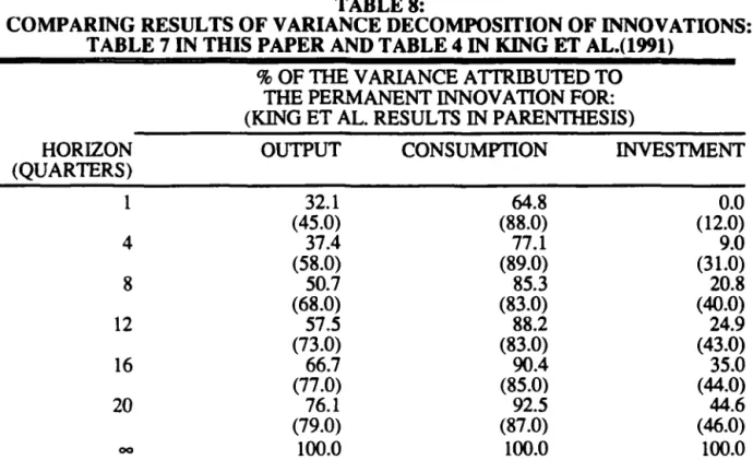
performed by King et al.(1991). Since both studies used the same data and sample period, the results are directly comparable and differences may be attributed to the use of different

methodologies. Results of our Table 7 are compared to their Table 4. Both are reported in Table

8. Since our trend-cycle decomposition was feasible, and imposed the common-cycle restrictions to recover these two components, any difference in results can be interpreted as a consequence of not imposing such restrictions to decompose the data. The major differences in results occur for small horizons (1-12 quarters): their method under estimates the contribution of the transitory

portion of output and investtnent. Moreover, for the 1-4-quarter horizon it over estimates the contribution of the permanent portion of consumption, which is reversed for larger horizons. The

biggest discrepancy happens for output: in their method, the permanent portion of output

explains almost 60% (70%) of output variance for the one-(two-)year horizon, whereas our result assigns about 40% (50%) to it.

The differences reported in Table 8 are enough to change the emphasis of the variance

decomposition results for output. It is clear that a much more considerable role should be attributed to sources of transitory noise. It is important to note that this result was obtained in a

framework where only real variables were considered, which in itself potentially limits the role of some so,srces of transitory noise, e.g., monetary policy. Another by-product of this analysis is

performing trend-cycle decompositions.

The imponance of transitory components of output was also reponed by Engle and Issler( 1993b) using a sectoral RBC medel. There, outputs of key sectors such as manufacturing and trade have most of their variance explained by transitory sources of noise. Cochrane( 1994)

also reports GNP having an imponant transitory component A similar general result is also achieved by King et al.(1991). They conclude that l i ••• V.S. data are not consistent with the view

that a single real permanent shock is the dominant source of business-cyc/e fluctuations. l i This

body of evidence goes against the claim in Nelson and Plosser( 1982) that permanent shocks are the most important source of noise for output. Although this is certainly true in the long run, the evidence points towards the imponance of transitory noise at business-cycle horizons.

For our tri-variate system, finding that permanent innovations for output and investrnent do not explain the bulk of their variance casts doubt on preductivity shocks being a major source of

output and investrnent fluctuations. In the RBC medel above, output, consumption and investrnent share a common stochastic trend, which is a multiple of the productivity processo Thus, if preductivity shocks are a major source of output fluctuation, we should find that

permanent innovations explain the bulk of output's variance, which is not the case. This result has several plausible interpretations. One is that transitory shocks from nominal variables are important For example, in the tradition of Friedman and Schwartz(1963), shocks to monetary

policy may lead the economy into recession. Romer and Romer(1990) present some evidence in

that direction. Another possibility is raised by King et al.(1991), who claim thatreal-interest-rate

shocks are a major source of output fluctuation through their effect on investrnent. Given that we found trans,itory shocks to be very important for investment fluctuations, this is cenainly an interesting path to explore.

-19-4.1 Explaining Unemployment's Fluctuations

A natural extension of our previous results is to examine causality between output-trend and -cycle innovations and unemployment. and the sources of variation for the latter using impulse-response functions and variance decomposition of forecast errors. A similar study was conducted by Blanchard and Quah(1989), building on the work of Evans(1987).

Before any analysis can be done, however, we should decide how to model unemployment: should it be modelled as an 1(0) or as an 1(1)? We follow Blanchard and Quah and treat it as 1(0).

There are good reasons why one should proceed in this way. First. it makes theoretical sense to impose the restriction that shocks should not have perrnanent effects on unemployment AIso, from the empirical point of view, the evidence in Nelson and Plosser( 1982) and in Perron( 1989) points in this direction.

Granger-causality-test results are reported in Table 9. At usual significance leveIs, there is evidence that both output trend and cycle innovations Granger-cause unemployment

Conversely, there is no evidence that unemployment Granger-causes either trend or cycle

innovations at alI usual significance leveIs. These results suppon the view that output shocks lead unemployment in the temporal sense, which, we believe, is agreed upon by many

business-cycle researc hers.

The second issue analyzed - impulse response functions and variance decomposition of

innovations of unemployment - is usually implemented using Vector Autoregressions (VAR's);

see Sims(1980). A VAR including eight lags of unemployment leveI, output-trend innovation,

and output-fycle innovation was frrst estimated. Although some authors modelled the

unemployment leveI as having a break in mean in 1974, e.g., Perron(l989), we do not allow for such a structural break in our V AR, since a structural break dummy is insignificant in the presence of the lags of our estimates of output-trend and -cycle innovations.

It is a well known fact that the ordering of innovations in the V AR affects the results of

variance decompositions and impulse-response functions. We chose the following order for innovations: output-trend frrst. output-cycle second and unemployment last12• This is the order

which makes the most theoretical sense. Interestingly enough, choosing different orders yielded the same qualitative results, although numerical differences existo We only analyzed

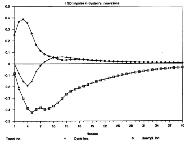
unemployment's response to different impulses. Results are plotted in Figure 9. The results are encouraging. First. an unemployment shock positively affects the unemployment leveI. Its effect peaks at the three-quarter horizon at about 40% of the original shock, dropping afterwards to be

negligible at the two-year horizon. Second, output-cycle innovation affects unemployment

negatively. Unemployment's response is greatest at the one-year horizon at about a fifth of the original shock. By the three-year horizon, unemployment's response is virtually zero. Third, output trend innovation affects unemployment negatively. Its effect is greatest at the five quarters

horizon at more than 40% of the size of the initial shock. Contrary to the effects previously discussed, effects of output-trend innovations decrease at a very low pace, affecting

unemployment in an enduring way. For example. at the four-year horizon, unemployment's

response is stiU about one fifth of the original shock.

l

(

12 This implies that contemporaneous shocks to output trend are present in both output-cycle innovation and unemployment. Also, contemporaneous shocks to output-cycle are present in unemployment.

FUNDAÇÃO GETÚLIO VARGAS Biblioteca Mário Henrique

Simonsen-

-21-From the impulse-response results, it seems that the only variable in our system that has a long-lasting effect on unemployment is output-trend innovation. This is not surprising, since trend innovations are the only shocks to have perrnanent effects on output. It is interesting to contrast responses from shocks to output trend with those to output cycle. Since the former have

bigger and more enduring effects on unemployment, firms may do labor hoarding, only

practicing generallay-offs of workers when they perceive shocks to have permanent effects on

production.

The results of the decomposition of FEV are presented in Table 10. We include horizons one through fony quarters. Up to the one-year horizon, unemployment shocks and output-cycle

shocks explain the bulk of FEV of unemployment. As the horizon increases, however, the only remaining important shock is that of output-trend innovation. For example, at the two-year horizon, output-trend innovations explain about 60% of unemployment's FEV. At the three-year horizon this proportion is up to about 70%. These results corroborate the evidence of the

impulse-response analysis, showing that, in the long run, only permanent shocks to output are

important for unemployment fluctuations.

At this point it is interesting to contrast our results with those of Blanchard and

Quah( 1989). They used a different way of decomposing output in trend and cycle, labelling trend

innovations as supply shocks and cyclical innovations as demand shocks13• The fact that they

used GNP instead of private per-capita GNP should not account for their impulse-response

results for unemployment being completely opposite to ours. In their data set, output-cycle innovations have bigger and more enduring effects on unemployment than output-trend

l

,

13 Sample periods are almost identical: they used 1950:2 through 1987:4 and we used 1951:2 through 1988:4.

innovations. Moreover, unemployment responses to the latter have the wrong sign up to the

fúth-quarter horizon and are negligible after that. Despite the differences in data, it seems hard to accept that shocks that have permanent effects on output (trend innovations) have little or no effect on unemployment, whereas those that have transitory effects on output (cycle innovations) have long-Iasting effects. The difference in results rnay be due to our use of a multivariate rather

than bi-variate system, or to the use of different decomposition methods. Again, this result may illustrate the efficiency gains associated with imposing both short- and long-run co-movement

restrictions in decomposing the data into trends and cycles.

4.2 Post-Sample Forecasts of

Per-C apita

Output, Consumption and

Investment

This last section compares post-sample forecasts of two econometric representations of our tri-variate system. The first is the Unrestricted VECM (UVECM), which does not take into

account short-run restrictions implied by the existence of common cycles. The second is the Restricted VECM (RVECM), which takes those restrictions into account. Sample estimates used data for output. consumption, and investment from 1947:1 to 1988:4. Post-sample

one-step-ahead forecasts for each representation were then calculated from 1989: 1 to 1991 :3,

comprising 11 quarterly observations.

Estirnation of the UVECM used eight lags for alllagged dependent variables and one lag

for the error-correction terms. Since it is a reduced-form, it was estimated by Least Squares. The

RVECM was estimated with the same lag structure of the UVECM, but imposing the

common-cycle restrictions in the system. As discussed in the Appendix, these restrictions require

.'

taking struétural relationships into account. Thus, the system was estirnated using FIML, a

-23-Forecasting results are plotted in Figures 10 through 12, as well as reported in Tab1e 11.

Table 11 shows two measures of forecasting performance. The frrst is the ratio of post-sample

Root Mean Square Errors (RMSE) of each dependent variab1e to its mean. It is a measure of the

forecasting performance of each equation of the system separately. The second is the determinant

of the Mean Square Error (MSE) matrix, a measure of the overal1 forecasting performance for

the system as a whole.

For the overall system. it is clear that the RVECM representation does better, although the

difference in MSE is not very large. For individual equations, the RVECM outperforms the

UVECM in forecasting output and consumption. The latter equation is the one where the

forecasting improvement is most remarkab1e. As is clear from Figure 11, the better performance

of consumption forecasts in the RVECM results from an apparent smoothing-out propeny of

these forecasts, while those of the UVECM are apparently more erratic. A1though the UVECM

outperforms the RVECM in forecasting investment, the numerical difference is negligib1e. As is

clear from Figure 12. one cannot distinguish any difference in forecasts just by 100king at the

ploto

It seems that the empirical results achieved here confrrms the theoretical prediction that

restricted estimation reduces MSE whenever true restrictions are imposed in estimation. In this

case. on average, efficiency gains outweigh the 10ss in bias, thus reducing MSE. Although a

smaller MSE can always

be

the consequence of a "good drawing." it is still encouraging to have

achieved it. As it seems, there is no reason not to improve forecasting performance whenever

possible. and the existence of common-cycle restrictions may allow for such an opportunity.

,I

5 Conclusions

This paper confrrms the prediction of the theoretical RBC model discussed in King, Plosser and Rebelo( 1988), that output, consumption and investment share both a common trend

and common cycles. Although common trends have been investigated and confmned before, e.g., King et al.( 1991), finding common cycles constitutes new evidence regarding such

important aggregate data set Despite the fact that the RBC model conforms well to the evidence

with respect to co-movement, it fails to conform to the prediction that the productivity shock is the major source of variation of the data. Indeed, it seems that transitory shocks are more important than previously suspected, given that they explain the bulk of the varianceof

investment and a substantial portion of the variance of output at the business-cycle horizon. Despite these results, the permanent shock explains a very large proportion of consumption variation, providing evidence of consumption smoothing over time.

Regarding the output-unemployment relationship, we found evidence that both transitory and permanent shocks to output Granger-cause unemployment Moreover, it seems that output's permanent shocks play a relatively important role in explaining unemployment' s fluctuations.

This result is not surprising, although it is the opposite of that found by Blanchard and

Quah( 1989). If there is a high cost associated with hiring/firing employees, one should expect

frrms to change labor units more frequently when facing permanent rather than transitory shocks

to production. If that is the case, our evidence is consistent with labor-hoarding practices by

frrms.

Finally, this paper establishes that ignoring common-cycle restrictions in multivariate data

,

-25-affect forecasting performance as well as precision in estimating trends and cycles, as shown

above. Therefore, testing for common cycles should always precede econometric estirnation

whenever short run co-movement restrictions are likely

to be

present.

l

6 References

Beveridge, S. and Nelson, C.R.(1981), "A New Approach to Decomposition ofEconomic

Time Series into a Permanent and Transitory Components with Particular Attention

to Measurement of the "Business Cycle" ,"

Journal of Monetary Economics, voI. 7,

pp. 151-174.

Blanchard, 0.1. and Quah, 0.(1989), "The Oynamic Effects of Aggregate Supply and

Demand Oisturbances,"

American Economic Review, voI. 79, pp. 655-673.

Bwns, A.F. and Mitchell, W.C.(1946),

"Measuring Business Cycles," New York: National

Bureau of Economic Research.

Campbell, J.Y. and Mankiw, N.G.(1987), "Permanent and Transitory Components in

Macroeconomic Fluctuations,"

American Economic Review, May 1987.

Campbell, J.Y. and Mankiw, N.G.(1990), "Permanent Income, Current Income, and

Consumption,"

Journal of Business and Economics Statistics, 8, pp. 265-279.

Cochrane, J.H.(1988), "How Big is the Random Walk in GNP?,"

Journal ofPolitical

Ecollomy, 96, pp. 893-920.

Cochrane, J.H.(1994), "Permanent and Transitory Components ofGNP and Stock Prices,"

Quarterly Journal of Economics, voI. 30, pp. 241-265.

Engle, R.F. and Granger, C.WJ.(1987), "Cointegration and Error Correction:

Representation, Estimation and Testing,"

Econometrica, voI. 55, pp. 251-276.

Engle, R.F. and Kozicki, S.(1993), ''Testing for Common Features,"

Journal of Business

and Ecollomic Statistics, voI. 11, pp. 369-395, with discussions.

Engle, R.F and Issler, J.V.(1993a), "Common Trends and Common Cycles in Latin

America,"

Revista Brasileira de Economia, voI. 47, 149-176.

Engle, R.F. and Issler, J.V.(1993b), "Estimating Sectoral Cycles Using Cointegration and

Common Features," Working paper 4529: National Bureau of Economic Research.

Fama, E.(1992), "Transitory Variation in Investment and Output,"

Journal of Monetary

Ecollomics, voI. 30, pp. 467-480.

Evans, G.(1987),

"Output and Unemployment Dynamics in the United States: 1950-1985,"

London: London School of Economics.

Friedman, M. and Schwartz, AJ.(1963),

"A Monetary History ofthe United States,"

Princeton: Princeton University Press.

HaU, R.E.( 1978), "Stochastic Implications of the Life Cycle - Permanent Income

Hypothesis: Theory and Evidence,"

Journal of Political Economy, 86, pp. 971-987.

Hall, R.E.(1989), "Consumption," In Robert Barro, Editor,

"Modem Business Cycle

Theory," Cambridge: Harvard University Press, 1989.

,

Johansen, S.(1988), "Statistical Analysis of Cointegrating Vectors,"

Journal ofEconomic

DYllamics alld Control, voI. 12, 231-254.

Johansen, S.(1991), "Estimation and Hypothesis Testing of Cointegration Vectors in

Gaussian Vector Autoregressive Models,"

Econometrica, voI. 59, pp. 1551-1580.

-27-King, R.G., Plosser, C.I. and Rebelo, S.( 1988), "Production, Growth and Business Cycles. lI. New Directions,"

Journal ofMonetary Economics,

voI. 21, pp. 309-341.

King, R.G., Plosser. C.I., Stock, lH. and Watson, M.W.(199l), "Stochastic Trends and Economic Fluctuations,"

American Economic Review,

voI. 81, pp. 819-840.

Lucas, R.E .• Jr.(1977), "Understanding Business Cycles,"

Carnegie-Rochester Conference

Series on Public Policy,

voI. 5, pp. 7-29. Amsterdarn: North Holland.

Muelbauer. 1.(1983), "Surprises in the Consumption Function,"

Economic Journal, 93

(suppI.), pp. 34-40.

Nelson. C.R. and Plosser, C.I.(1982), "Trends and Random Walts in Macroeconomic Time Series,"

Journal ofMonetary Economics,

vol. 10, pp. 139-162.

Osterwald-Lenum, M.(1992). Quantiles ofthe Asymptotic Distribution ofthe Maximum Likelihood Cointegration Rank Test Statistics,"

Oxford BuJletin of Economics and

Statistics,

voI. 54,461-472.

Perron, P.(1989), "The Great Crash, the Oil Price Shock and the Unit Root Hypothesis,"

Econometrica,

voI. 57, pp. 1361-1402.

Prescott, E. C. (1986), "Theory Ahead of Business-Cycle Measurement,"

Carnegie-Rochester Conference Series on Public Policy,

voI. 25, pp. 11-44. Amsterdarn: North Holland.

Rao, C.R.(1973),

"Linear Statisticallnference,"

New York, Wiley.

Romer, O.H. and Romer, C.O.(1990), "The Monetary History After Twenty-Five Years: New Evidence on the Money-Output Relationship,"

Brookings Papers,

vol. 21, pp. 149-199.

Sims, C.A.(1980), "Macroeconomics and Reality,"

Econometrica,

48, pp. 1-48. Stock, lH. and Watson, M.W.(1988), "Testing for Common Trends,"

Journal ofthe

American Statistical Association,

voI. 83, pp. 1097-1107.

Vahid, F. and Engle, R.F.(1993), "Common Trends and Common Cycles,"

Journal of

Applied Econometrics,

voI. 8, pp. 341-360.

Watson, M.W.(1986), "Univariate Detrending Methods with Stochastic Trends,"

Journal

of Monetary EcolJomics,

vol. 18, pp. 49-75.

Y oon, G.( 1992), "Common Stochastic Trends in Cointegrated Systems: Representation, Estirnation and Testing," Unpublished manuscript, University of Califomia, San Oiego.

Zeldes, S.(1989), Consumption and Liquidity Constraints: An Empirical Investigation,"

Journal of Political Economy,

voI. 97, pp. 305-346.

l

-28-7 Appendix

7.1 Co-Movement Restrictions in Dynamic Models

Before diseussing the c!ynarnie representation of the data. and the trend-cycle

decomposition method used, we present the definitions of common trends and common cycles;

for a full diseussion see Engle and Granger(I987) and Vahid and Engle(1993) respectively. First, we assume that y, is a 11 - veetor of I( 1) variables, with the following stationary Wold

representation (MA( 00»:

Ily,

=

C (L)E, (A.I)

-where C(L) is a matrix polynomial in the lag operator, L, with C(O) =1",

.I.

jl Cjl < 00 and E, is

) .. 1

a 11 X 1 vector of stationary one-step-ahead linear forecast errors in y, given inforrnation on

lagged values of y,. We ean rewrite equation (A.I) as:

Ily,

=

C(1)E,

+

IlC·(L)E, (A.2)

where

c·

.

= _{. .}

I.

-C. ₎ 'Vi. In Particular C~ =1" -C(1)

) >.

If we integrate both sides of equation (A.2) we get:

-.' y, = C(1)

I.

E,_s

+

C "(L)E, s-o (A.3) ..

=

T, + Ct

-29-Equation (A .3) is the multivariate version of the Beveridge-Nelson trend-cycle representation

(Beveridge and Nelson( 1981». Series

y,

are represented as sum of a random walk part T, which is called the "trend" and a stationary part C, which is called the "cycle".

Definition 1: The variables in y, are said to have common trends (or coilltegrate) ifthere are r

linearly independent vectors, r

< 11,

stacked in a r x n marrix a', with the property that:

a'CO) = O.

rXII

Definition 2: The variables in y, are said to have common cycles if there are s linearly

independent vectors, s

S Il -

r, stacked in a s

x n

marrix õ.', with the property that:

õ.'C"(L)

=

O.

IXII

Thus. cointegration and common cycles represent restrictions on the elements of C (1) and

C"(L)

respectively.

We now discuss restrictions to the dynamic autoregressive representation of economic time series arising from cointegration (common trends) and common cycles. First, we assume that y, is generated bya Vector Autoregression (VAR):

.'

(

Engle and Granger(1987) show that. if and only ifthe elements of y, eointegrate, the

system (A.4) ean be written as a Vector Error-Correetion model (VECM). This shows the existenee of eross-equation restrietions in the V AR given by eointegration:

where

y

and

a

are full rank matriees of order

n

x

r, r

is the rank of the eointegrating spaee,

p p

I -

r

ri

=

ya.',

and

r;

= -

r

ri'

j

=

1, ... ,p -1. Given the eointegrating vectors stacked in

ial i=j+l

a',

they show that (A.5) parsimoniously encompasses (A.4). Oearly, given the parameters in

(A.5), one ean recover those of (A.4) by the formulae above. Moreover, the latter has n2• p

pararneters in the eonditional mean, while the former has n 2(p - 1)

+

n . r. Thus, n (n - r) fewer pararneters, sinee r < n.

Vahid and Engle( 1993) show that the dynamie representation of the data y, may have additional eross-equation restrietions if there are eommon eyeles. To see this, recall that the eofeature veetors

<i;',

staeked in an s

x

n matrix

ã'.

eliminate all lhe serial eorrelation in lly,. Now, rotate

ã

to have an

s

dimensional identity sub-matrix as follows:

_ [1,,]

a

= _. ,

~,,-,»('

thus.

ã'

lly, ean be looked at as s pseudo-struetural form equations for lhe first s elements of lly,.

Complete the system by adding the uneonstrained VECM equations for the remairiing n-s elements o( lly, to get the following system:

[ Is

ã..']

O

I ~Y, 11-' (II-')X. -31-= [ SX(!+r) ] •• •• •

rI ... rp_l'Y

~Y'-I +

v,.

(A.6) ~Y,-p+1

,

aY'_1

where

1;.

and

f

represent the partitions of

1;

and 'Yrespectively, corresponding to the bottom

[

I.

ã..']

n -s

reduced form VECM equations, and v, =

o

111_' E,.

(II-.)X$

[

I.

ã.

0 ' ]

It is easy to show that (A .6) parsimoniously encompasses (A .5). Since

o

1 11 _. is

(II-')X'

invertible, it is possible to recover (A .5) from (A .6) by inverting it. Notice however that the latter

has s (Ilp

+

r) - s (n - s ) fewer pararneters.

7.2 Trend-Cycle Decomposition

We now discuss the trend-cycle decomposition used here; for a fuIl discussion see Vahid and Engle(1993). Recall equation (A.3):

-y,

= C(1)

I:

E,_s

+

C·(L)E, (A.3)

.-0

,

;

T,

Consider now the following special case:

n

= r

+

s.

Stack the cofeature and the cointegrating combinations:

(A.7)

The Il X 11 matrix A =

[~1

has full rank and therefore is invertible. Partition the

columns of the inverse accordingly as A-I =

[ã-

I al

and recover the common-trend common-cycle decomposition by pre-multiplying the cofeature and cointegrating combinations byA-1

:

(A.8)

implying T, =

ã-ã'y,

and

C,

=

a-a'y,.

Notice that the frrst term in (A .8) loads into the cofeature-vector linear combinations, while

the second loads into the cointegrating-vector linear combinations. Indeed, this illustrates that the

frrst are

trelld generators,

while the second are

eyele generators

in this decomposition.

l

-33-7.3 Tables and Figures

TABLE I:

COINTEGRATING RESUL TS USING JOHANSEN'S(I988) TECHNIQUE

EIGENV ALUES TRACETEST

(Ili ) -T

I.

10(1 - J..l.)

j S.i J

0.01886 3.06

0.07726 16.01

0.13944 40.18

Estimated Normalized Cointegrating Space:

Ao, = ( -1.06 1

O)

a -1.01 O 1

Test of Restrictions in the Cointegrating Space:

X2(2)

=

3.856, p-value

=

0.1454. l ( CRITICAL NULL VALUE HYPOTHESES AT5% 3.76 3 at most 2 coint. vectors 15.41 3 at most 1 coint. vectors 29.68 3 at most O coint. vectors

-34-TABLE2:

CANONICAL CORRELATION ANAL YSIS COMMON-CYCLE TESTS

SQUARED Prob >

x.

2(d) _{Prob.>F NTJLL HYPOTHESES}

CANONICAL (d) CORRELA TIONS (p;)

0.4892 >0.0001 0.0001 Current and alI smalIer (p;) are zero (78)

0.2860 0.004 0.0226 Current and alI smaller (pj) are zero (50)

0.1544 0.3200 0.4651 Current and alI smaller (Pi) are zero (24)

TABLE3:

COINTEGRATION AND COFEATURE SPACES

l

,

COINTEGRA TING VECfOR 1 COINTEGRA TING VECFOR2 COFEATURE VECfOR 1 Y -1.00 -1.00 -1.37 DATA

c

i 1.00 O O 1.00 -2.83 1.00

-35-TABLE4:

COMMON FACfORS REPRESENTATION FACTO R LOADINGS OF NORMALIZED FACfORSa

FACfORS

VARIABLE CYCLEl CYCLE2 -COMMON

c-y

i-y

y -0.0223 0.0127

c

0.0032 0.0127

i

-0.0223 0.0554 Notes: (a) To have unit variance.

TABLE5:

CORRELATION MA TRIX OF FACfORS

CYCLE 1 (p-value) CYCLE2 (p-value) COMMON TREND l ( (p-value) CYCLEl CYCLE2

c-y

i-y

1.00 -0.3070 (0.0001) 1.00 TREND -0.0930 -0.0930 -0.0930 COMMON TREND 0.5669 (0.000 1) -0.0169 (0.828) 1.00

TABLE6:

TRENDS AND CYCLES AS LINEAR COMBINATIONS OFTHE DATA-TRENDS VARIABLE Y c y 0.42 0.87 c 0.42 0.87 i 0.42 0.87 CYCLES VARIABLE _Y c v 0.58 -0.87

c

-0.42 0.13 i -0.42 -0.87

Notes: (a) A constant is also used to obtain a zero mean cycle.

TABLE 7:

VARIANCE DECOMPOSITION OF INNOVATIONS AT BUSINESS CYCLES HORIZONS

% OF'IHE V ARIANCE ATIRIBUTED TO

'lHE PERMANENT INNOVATION FOR:

i -0.29 -0.29 -0.29 i 0.30 0.30 1.30 HORIZON (QUARTERS)

OUTPUT CONSUMPTION INVESTMENT

1 4 8 12 16 20

-32.1 37.4 50.7 57.5 66.7 76.1 100.0 64.8 77.1 85.3 88.2 90.4 92.5 100.0 0.0 9.0 20.8 24.9 35.0 44.6 100.0 Note: Since trend and cycle innovations are correlated, we denote transitofY. innovation the portion of the cycle innovation which is orthogonal to the trend innovation. The permanent mnovation will then be the trend innovation prus the part of the cycle innovation eXp'lained by the trend innovation. This orthogonalization method IS identical to ordering the trena innovatlon

fIrst, i.e. cycle innovations contaming the trend innovation and not vice-versa. l

-37-TABLE8:

COMPARING RESULTS OF VARIANCE DECOMPOSITION OF INNOVATIONS: TABLE 7 IN THIS PAPER AND T ABLE 4 IN KING ET AL.(1991)

HORIZON (QUARTERS) l ( 1 4 8 12 16 20 00

% OF TIffi V ARIANCE A ITRffiUTED TO THE PERMANENT INNOVA TION FOR: (KING ET AL. RESUL TS IN P ARENTHESIS)

OUTPUT CONSUMPTION INVESTMENT

32.1 64.8 0.0 (45.0) (88.0) (12.0) 37.4 77.1 9.0 (58.0) (89.0) (31.0) 50.7 85.3 20.8 (68.0) (83.0) (40.0) 57.5 88.2 24.9 (73.0) (83.0) (43.0) 66.7 90.4 35.0 (77.0) (85.0) (44.0) 76.1 92.5 44.6 (79.0) (87.0) (46.0) 100.0 100.0 100.0

TABLE9:

GRANGER CAUSALITY TESTS FOR UNEMPLOYMENT,

OUTPUT TREND INNOVATION, AND OUTPUT CYCLE INNOVATION (MEAN VERSION)

P-V ALUES FOR GRANGER CAUSAUTY F-TESTS IN A TRI-VARIATE VAR

VAR ORDER FROM TREND FROM CYCLE FROM UNEMPL. FROM UNEMPL. (LAGS) TO UNEMPL. TO UNEMPL. TO TREND TO CYCLE

1-8 0.00007 0.00475 0.98022 0.83328

TABLE 10:

VARIANCE DECOMPOSITION OF INNOVATIONS IN VAR WITH UNEMPLOYMENT, OUTPUT TREND INNOV ATION,

AND OUTPUT CYCLE INNOVATION

% OF TIfE V ARIANCE A TTRIBUTED TO INNOVATION IN:

HORIZON (QUARTERS)

OUTPUT TREND OUTPUT CYCLE UNEMPLOYMENT

l ( 1 4 8 12 16 20 30 40 10.1 35.3 57.6 66.8 69.5 70.8 71.9 72.1

0.0

8.1 5.9 5.0 4.9 4.8 4.7 4.7 89.9 56.7 36.5 28.2 25.6 24.2 23.4 23.2

DEPENDENT VARIABLE Y

c

i I MSEI l

,

-39-TABLE 11:

POST -SAMPLE FORECASTING RESUL TS FOR THE RVECM AND UVECM REPRESENT ATIONS

MEANSQUAREERROR RA TIO MSE TO MEAN OF (MSE) DEPENDENT V ARIABLE (%)

RVECM UVECM RVECM UVECM

5.95E-05 6.12E-05 1.96 1.98 4.19E-05 5.08E-05 1.47 1.62 4.59E-04 4.58E-04 5.43 5.42 3.44E-24 4.02E-24

•

•

Figure 1

Per-Capita Private GNP, Private Consumption and Fixed Investment

•

•

•

•

• •

•

cn O" o c:::: 3 2 1

o

NBER Recessions Shown

~ ...

~

r

'-...

/

--

---'~-,..-..,,-

----

f-

-~V ~

v~ ["\.V

--.."

-

---

:.--

---

r-

---

--"---v...",...---

-v

-

,-"

,--- lr-

/

--

--

. /

/

'"

,

_ . / V' , _i--'

-

l/

/----

.--./ ,"'- -V'

,V -

r--,r

_'-' 1/ I I I I I I I I I I I I I I I I I I I I I I I I I I I I I I I I I I I I I I I 4445555555555666666666677777777778888888888 7890123456789012345678901234567890123456789 ,t (

Output

---_.~

- -

- - Investment

•

•

•

•

2.9

•

_2.8 2.7 '" 2.6 c> o - 2.5 c:

..

-2.4 2.3 2.2 2.1

•

• •

•

•

Figure 2

Per-Capita Private GNP and its Trend

NBER Recessions Shown

V

I"~

_\

V

J

'\

~

,-~ '" f I 7" I

~V

.... Ir'

r

\.

[7

~

..r-1'- ." ~ I I I I I I I I I I I I I I I I I I I I I I I I I I I I I I I I I I I I I I I I 444 5 5 555 5 555 5 6 666 6 6 6 6 6 6 777 7 777 7 7 7 888 8 8 888 8 8 7890123456789012345678901234567890123456789 l

,

YEAR GNP=solid Trend=broken

·

"

•

2.7

•

2.6 2.5 2.4 rn ~ 2.3 c 2.2

•

_2.1 2.0 1.9 1.8

•

..

•

•

•

...J _, , , : -i I

l

Figure 3

Per-Capita Private Consumption and its Trend

NBER Recessions Shown

IV

, , I i I I

V

-'"

V

1-'-1_ I--'"

r-..:

:

I

, _V~ i

V

t"- _,

n

~

]~

_, I i , I I I I i I I I I I I I I I I I I I I I I I I I I I I I I I I I I I I I I 444 5 5 5 5 5 5 5 5 5 5 6 666 666 6 6 6 7 7 7 7 7 7 7 7 7 7 8 8 8 8 8 8 8 8 8 8 7890123456789012345678901234567890123456789 YEAR Consumption=solid Trend=broken l (

•

• .ti

•

1.4

•

1.3 1.2 1.1 Cf) ~ 1.0 c: 0.9

•

..J 0.8 I

•

..

•

•

•

0.7 0.6 0.5

Figure

4

Per-Capita Fixed Investment and its Trend

NBER Recessions Shown

444 5 5 5 5 5 5 5 5 5 5 6 666 6 6 6 6 6 6 7 7 7 7 7 7 7 7 7 7 888 888 8 8 8 8 7890123456789012345678901234567890123456789 I ( YEAR Investment=solid Trend=broken

•

•

0.09 0.08 0.07 0.06 0.05 0.04 0.03 ~ 0.02 o 0.01 c::; 0.00 ... - -0.01 -0.02 -0.03 -0.04 -0.05 -0.06 -0.07

Figure 5

Cyele in Per-Capita Private GNP

NBER Reeessions Shown

-0.08 ~~~~~~~~~~~~~~~~~~~~~~~~~~~~

•

•

4445555555555666666666677777777778888888888 7890123456789012345678901234567890123456789 .' ( YEAR

•

·

..

•

•

rn O> o

•

•

•

0.03 0.02 0.01 0.00 -0.01 -0.02

Figure 6

Cyele in Per-Capita Private Consumption

NBER Reeessions Shown

4445555555555666666666677777777778888888888 7890123456789012345678901234567890123456789

l

(

• 4

•

0.16 0.14

•

0.12 0.10 0.08 0.06 0.04

'"

0.02 C'> 0.00 o - -0.02

I

~

-0.04

J

..

--0.06 -0.08 -0.10 -0.12 -0.14 -0.16 -0.18

Figure 7

Cycle in Per-Capita Fixed Investment

NBER Recessions Shown

-0.20 ~~~~~~~~~~~~~~~~~~~~~~~~~~~~ • 4445555555555666666666677777777778888888888 7890123456789012345678901234567890123456789

•

•

•

l

,

YEAR