Comparisons of the Adsorption Equilibrium of Benzene Derivatives in Reversed-Phase Liquid Chromatography

(1)

Tiago Pereira dos Santos

Bachelor in Chemical and Biochemical Engineering

Comparisons of the Adsorption Equilibrium of

Benzene Derivatives in Reversed-Phase Liquid

Chromatography

Dissertation submitted in partial fulfillment of the requirements for the degree of

Master of Science in

Chemical and Biochemical Engineering

Adviser: José Paulo Barbosa Mota, Full Professor, NOVA University of Lisbon

Co-advisers: Andreas Seidel-Morgenstern, Full Professor,

Max Planck Institut for Dynamics of Complex Technical Systems

Ju Weon Lee, PostDoc,

(2)

(3)

Comparisons of the Adsorption Equilibrium of Benzene Derivatives in Reversed-Phase Liquid Chromatography

(4)

(5)

First of all, I would like to thank to Professor Andreas Seidel-Morgenstern for allow-ing me to work here in the MPI for Dynamics of Complex Technical Systems, providallow-ing me all of the resources available in the MPI so I could improve my research and produc-tivity and showing a great concern about my progresses and my results. Second, I would like to thank to my supervisor, Ju Weon Lee, for showing a tremendous amount of pa-tience teaching me everything I needed to succeed in this work, for showing an amazing availability when it came to questions, doubts, dead ends, suggestions, etc... Everything I needed, he always did everything in his power to help achieve my goal, finishing this thesis.

I also want to thank to my parents, Isabel Santos and Vítor Santos, for allowing and helping me to go in this journey, it was not an easy one... They, along with my brother, Pedro Santos, were always there for me and supported me with words of advice, and sometimes just words. My grandparents of my father side, Judite Santos and Bento San-tos, who are not among the living anymore, for providing me all the conditions available to them to ensure I succeeded in the past five years. To my grandparents from my mother side, Jaime Pereira, who is also not between us, e Carminda Pereira, for helping me, espe-cially finanespe-cially, throughout these five years so I could stay in college with a comfortable life.

Now, I want to thank my girlfriend, Marta Pereira, whom I love very much, for being the person she is, always giving me the words I needed to hear to help me staying focused in what I had to do and always reminding me that I’m following this path so we could have a good life together, but especially because I love what I do, I’m following this path because I want to.

I would like to thank all my friends, Edgar Teixeira, Rúben Anjos, Rita Paiva and several more, that accompanied me throughout this long, and really tough, journey, they are people whom I’ll never forget, and with most of them I’ll continue to stay in touch.

(6)

(7)

A b s t r a c t

(8)

(9)

R e s u m o

(10)

(11)

C o n t e n t s

Contents xi

List of Figures xiii

List of Tables xv

List of Equations xvii

Acronyms xix

Nomenclature 1

1 Introduction 3

1.1 Chromatography: from Ancient to Modern Times . . . 3

1.2 Normal-/Reversed-Phase Chromatography . . . 3

1.3 Liquid Adsorption - The Isotherm Models . . . 4

1.3.1 Multi Component Isotherms . . . 6

1.3.2 A Novel Generic Model: the Multi-Layer Multi-Component Isotherm 7 1.4 Experimental Approaches . . . 8

1.4.1 Static Methods . . . 8

1.4.2 Dynamic Methods . . . 8

2 Mathematical Descriptions 11 2.1 Frontal Analysis . . . 11

2.2 Linear Isotherm . . . 12

2.3 Langmuir Isotherm . . . 12

2.4 Freundlich Isotherm . . . 13

2.5 BET Isotherm . . . 13

2.6 Multi-Component Isotherms . . . 14

2.6.1 Extended Langmuir Isotherm . . . 14

2.6.2 Ideal Adsorbed Solution Theory . . . 14

2.6.3 MLMC Model . . . 15

(12)

CO N T E N T S

4 Data Analysis 23

4.1 Pure Components Isotherms . . . 23

4.1.1 Valerophenone . . . 24

4.1.2 Butyl Benzoate . . . 26

4.1.3 tert-Butylbenzene . . . 27

4.1.4 Parameter Estimation . . . 28

4.2 Multi-Component Isotherms . . . 31

4.2.1 Butyl Benzoate and tert-Butylbenzene . . . 33

4.2.2 Valerophenone and tert-Butylbenzene . . . 37

4.2.3 Parameter Estimation . . . 40

4.3 Experimental Validation . . . 43

5 Conclusions 49

Bibliography 51

(13)

L i s t o f F i g u r e s

1.1 The four most common Isotherm behaviours [19] . . . 5

1.2 Elution Profiles [25] . . . 6

1.3 Example of a single step FA experiment [15] . . . 9

1.4 Example of a multi-step FA [15] . . . 10

2.1 Frontal Analysis procedure for accumulated mass calculation [6] . . . 11

4.1 Molecular Structure of the three components used . . . 23

4.2 Valerophenone Raw Data . . . 24

4.3 Valerophenone Isotherm Data . . . 25

4.4 Butyl Benzoate Raw Data . . . 26

4.5 Butyl Benzoate Isotherm Data . . . 26

4.6 tert-Butylbenzene Raw Data . . . 27

4.7 tert-Butylbenzene isotherm data . . . 27

4.8 MLMC Model fitted for BBzt and tBBz . . . 29

4.9 MLMC Model fitted for VPhn and tBBz . . . 29

4.10 BCs for BBzt and tBBz with 1/1 Ratio . . . 33

4.13 Isotherm data for BBzt and tBBz . . . 36

4.14 BCs for VPhn and tBBz with 1/1 Ratio . . . 37

4.17 Isotherm data for VPhn and tBBz . . . 40

4.18 Fitted model for BBzt and tBBz . . . 41

4.19 Fitted model for VPhn and tBBz . . . 42

4.20 Cross-check for VPhn and tBBz . . . 44

4.21 Cross-check for BBzt and tBBz . . . 45

4.22 Cross-check for VPhn and tBBz . . . 46

(14)

(15)

L i s t o f Ta b l e s

3.1 Column Properties . . . 20

3.2 Solutions Concentrations for Single Components . . . 20

3.3 Concentrations used for Binary Mixtures . . . 21

4.1 Estimated parameters for each fitting . . . 30

(16)

(17)

L i s t o f E q ua t i o n s

1.1 Batch Method mass balance [15] . . . 8

2.1 Frontal Analysis mass balance [6] . . . 12

2.3 Linear Isotherm [6] . . . 12

2.4 Langmuir Isotherm [19] . . . 12

2.5 Freundlich Isotherm [21] . . . 13

2.6 BET Isotherm [19] . . . 13

2.7 Extended Langmuir Isotherm [1] . . . 14

2.8 Extended Langmuir Isotherm with competition term [1] . . . 14

2.9 Interaction factor calculation [1] . . . 14

2.14 IAST calculation method [2] . . . 15

(18)

(19)

Ac r o n y m s

BBzt ButylBenzoate. BC Breakthrough Curve.

ELI Extended Langmuir Isotherm.

FA Frontal Analysis.

FACP Frontal Analysis by Characteristic Point.

HPLC High Performance Liquid Chromatography.

IAST Ideal Adsorbed Solution Theory.

IUPAC International Union of Pure and Applied Chemistry.

LC Liquid Chromatography. LSQ Least Squares.

MLMC Multi-Layer Multi-Component.

NPLC Normal-Phase Liquid Chromatography.

RPLC Reversed-Phase Liquid Chromatography.

tBBz tert-ButylBenzene.

TLC Thin-Layer Chromatography.

(20)

(21)

N o m e n c l a t u r e

Csat saturation concentration (mg/ml)

C0 concentration of the feed (mmol/ml)

ci concentration of the componenti (mmol/ml)

c_ieq concentration of componentiin solution after equilibrium (mg/ml)

c_iinit initial concentration of componenti(mg/ml)

K1,i first constant of componenti(min)

K2,i second constant of componenti(min)

Macc accumulated moles of solute inside the column (mmol)

mads moles of adsorbent (mg)

n number of layers

q moles of solute per volume of stationary phase (mmol/ml)

qeq_i mass concentration of component i in volume of adsorbent after equilibrium (mg/ml)

qMAX maximum adsorbed moles in a monolayer per volume of adsorbent (mmol/ml)

t0,f front dead time (min)

t0,r rear dead time (min)

t_{inf l,f} front (or loading) inflexion time (min)

tinf l,r rear (or elution) inflexion time (min)

V0 column void volume (ml)

V0,sys void volume of the system without column (ml)

Vads volume of adsorbent (ml)

(22)

(23)

C

h

a

p

t

e

r

1

I n t r o d u c t i o n

1.1 Chromatography: from Ancient to Modern Times

The experiment which gave birth to Chromatography is well known. In 1902, the Russian botanist M. S. Tswett managed to separate plant pigments with proper solvents and adsorbents [7, 14]. In former studies of his work about the separation ofα- and

β-carotenes, it was seen that he tried hundreds of combinations of stationary and mobile phases and understood that the most important characteristics of the chromatographic process are the purity of the adsorbent and the particle size distribution [7]. He also knew the three ways to realize a chromatographic process: elution, frontal analysis and displacement.

30 years had to pass before someone could reproduce Tswett experiment, accom-plished by Kuhn and Lederer. After that, the development of preparative and adsorption chromatography started to grow at a high rate.

1.2 Normal-/Reversed-Phase Chromatography

According to the IUPAC, liquid chromatography (LC) is a mean of separating compo-nents in mixtures by distributing them between two phases, in which one of the phases moves freely (mobile phase) through the other, which is fixed (stationary phase), and it’s called liquid chromatography because the mobile phase is a liquid. Since its invention, many types of LC were born, such as microbore LC, preparative LC and high performance LC (HPLC), but the emphasis will be in the normal- (NPLC) and reversed-phase (RPLC) chromatography.

(24)

C H A P T E R 1 . I N T R O D U C T I O N

and it’s still the predominant technique for thin-layer chromatography (TLC) and low-pressure dry-column LC. Its main characteristic is the stationary phase being more polar than the mobile phase. Since the stationary phase (usually inorganic adsorbents like silica gel) is more polar than the mobile phase, the retention time increases when the polarity of the mobile phase decreases and vice-versa. After the appearance of RPLC, NPLC started losing ground because RPLC off_{ers much more selectivity, even with mixtures in which} the two compounds have minor diff_{erences in their molecule sizes. That’s why RPLC is} usually chosen when working with HPLC. Either way, NPLC is much better in isomers separation [8].

In reversed-phase LC the stationary phase is less polar than the mobile phase, quite hy-drophobic, so the retention time increases when the polarity of the mobile phase increases and vice-versa. In RPLC, the separation is determined almost entirely by molecular size and polarity, so it easily separates molecules with similar polarity but diff_{erent carbon} numbers. However, since the stationary phase is hydrophobic (usually C18 or C8), the mobile phase cannot be only water. If only water is used, chances are high that the solutes never elute from the stationary phase, ruining the analysis. Usually, at least 5-10% of organic solvent (methanol, acetonitrile and tetrahydrofuran) has to be mixed with water.

With all these chromatographic methods, the main problem is to choose the best combination for the process studied, so it’s important to answer these simple questions: is it needed only organic solvents as mobile phase? Are the components isomers? Is the objective separation or analysis? After answering these main questions, it’s much easier to choose the best method.

1.3 Liquid Adsorption - The Isotherm Models

In chromatographic processes, the understanding of what happens inside the column is critical. Each component has diff_{erent behaviours, regarding retention time, type of} adsorption (monolayer or multilayer) and affi_{nity with solid phase, with di}ff_erent pack-ings, diff_{erent mobile phases and mobile phase ratios (if they are a mixture). If a Frontal} Analysis was to be performed with a broad range of concentrations and after the calcu-lation of the adsorbed masses in the stationary phase, one could plot the adsorbed mass concentration in the solid phase, q0, as a function of the concentration of the inlet,C0, and obtain several types of curves. Below are represented the most common curves:

(25)

1 . 3 . L I Q U I D A D S O R P T I O N - T H E I S O T H E R M M O D E L S

Figure 1.1: The four most common Isotherm behaviours [19]

Figure 1.1 (a) is the simplest case of adsorption, when the adsorbed mass is directly proportional to the bulk concentration. In very dilute concentrations, all compounds follow this behaviour, however it’s not usual to see a compound with linear behaviour in a broad range of inlet concentrations.

The curve presented in Figure 1.1 (b) has a concave shape, meaning, in low concentra-tions, the increase inq0is practically linear, but as the concentration of the inlet increases even more,q0reaches a maximum, the saturation concentration of solute in the station-ary phase. This type of curve is usually called the Langmuir Isotherm since it was Irving Langmuir who developed the first model that described very well this curvature. How-ever, his work was based in a theoretical background and several assumptions had to be made to reach a good mathematical model and, in solid-liquid adsorption, many times some of those assumptions are invalid and the model is not well fitted to the experimental data.

Figure 1.1 (c) is first concave and then turns to convex shape. It shows that it has Langmuirian behaviours for lower concentrations, but if the concentration continues to increase, it suddenly surpasses the maximum adsorbed capacity. In fact, in lower concentrations it occurs only monolayer adsorption, which means, the solute is only adsorbed directly in the solid phase surface, and in higher concentrations the adsorption starts to be multilayer, all the active sites are covered with solute and now the molecules adsorb on top of the previously adsorbed molecules. It’s most commonly called a BET behaviour. The BET Isotherm Model can describe, depending on it’s parameters, the concave shape, the convex shape (monolayer adsorption) and multilayer adsorption.

(26)

to reach a saturation concentration. Of course it only applies in C0 ranging from 0 to

Csat. The most common model that describes this adsorption behaviour is the Freundlich Model, despite its empirical nature. This model can describe three types of shape: the concave, the convex and the linear shape, depending on the values of it’s parameters. Furthermore, the convex shape is also usually called an anti-Langmuirian shape.

Figure 1.2: Elution Profiles [25]

In Figure 1.2 is seen the most common isotherms (Langmuirian and anti-Langmuirian) and their elution profiles. Figure 1.2 (b) shows a very steep front and a diff_{use rear. It’s} logic because components which follow a langmuirian behaviour tend to adsorb more in lower concentrations. That can be seen in Figure 1.2 (a) where the slope, in lower concentrations, is much bigger than in higher concentrations. It means that, when the step response is interrupted, the concentration starts to decrease and the retention time increases, forming the "long tail" seen in the figure. Figure 1.2 (d) is exactly the opposite, has a very diff_{use front and a very sharp rear. The way of thinking is the same as before,} only that is exactly the inverse, since it adsorbs more in higher concentrations, when the step response is turned on it forms the "long tail" and when it’s shut down the retention time decreases abruptly, forming that very sharp rear.

1.3.1 Multi Component Isotherms

1.3.1.1 Extended Langmuir Isotherm

The extended langmuir isotherm (ELI) was first developed in 1930 by Butler and Ockrent. This model considers competitive behaviour between species and was based in all the langmuir model assumptions. After this model development, several researchers modified the ELI to try and have more accurate and precise approaches for description

(27)

1 . 3 . L I Q U I D A D S O R P T I O N - T H E I S O T H E R M M O D E L S

of binary mixtures, such as Jain and Snoeyink in 1973 and [9]. One setback about these models is that they always assume only monolayer adsorption.

1.3.1.2 Ideal Adsorbed Solution Theory and some Derivations

The ideal adsorbed solution theory (IAST) is a powerful tool for predicting multi-component isotherms with only the single multi-component isotherms. The biggest model assumption is that the adsorbates are thermodynamically ideal, which means that, for two components A and B, the interactions between A and B are no diff_{erent than those} between A and A and B and B. With this assumption and good isotherm models to describe the pure components’ behaviours, the mixture equilibrium data can be directly predicted from the pure component data. Usually the predictions are quite good, but a major setback is that it needs, for each combination of concentration points of A and B, to solve numerically the equations associated with this model. To get very good equilibrium mixture data, the numerical calculation can take lots of time.

There are several derivations of the IAST. Among them are the non-ideal adsorbed solution theory (NIAST), the heterogeneous ideal adsorbed solution theory (HIAST) and the predictive real adsorbed solution theory (PRAST). Several works were published, [3, 23, 24] regarding these new derivations to try and improve the IAST.

1.3.2 A Novel Generic Model: the Multi-Layer Multi-Component Isotherm

Until now, there’s a lack of models that can describe correctly the behaviour of two components in a liquid adsorption process. Some studies were made using the Extended Langmuir Isotherm and some modified models [1] but with no good results. Another study was performed using a modification of the Extended Langmuir Isotherm that was successful to predict competition between species and active sites [9]. However, the latter is basically a direct application of the Extended Langmuir Model, meaning that it assumes only monolayer adsorption, an assumption that is not valid in many cases in Liquid Adsorption.

In the attempt to develop a model that can explain some phenomena that the known models can’t, a research group from Max Planck Institut for Dynamics of Complex Tech-nical Systems led by Professor Andreas Seidel-Morgenstern presented in 2016 in the Fun-damentals of Adsorption (FOA) Conference the Multi-Layer Multi-Component (MLMC) Isotherm Model [10], a model based entirely on a theoretical background.

(28)

1.4 Experimental Approaches

The adsorption phenomenon varies with the mobile and stationary phases and with the component being studied. Hence, there’s no way to determine adsorption isotherms in a theoretical way only, it’s needed lots of experimental work. Since Chromatography was born, a significant number of experimental methods were developed, with the static methods at first and more recently the dynamic methods.

The main focus of this work resides in the dynamic methods, so the static methods will not be referred in high detail.

1.4.1 Static Methods

To measure adsorption isotherms with static methods, only the initial and the equilib-rium concentrations are needed,c_i(t= 0) andc_i(t→ ∞_{) respectively.}

1.4.1.1 Batch Method

In the Batch Method, a vessel is loaded with adsorbent of massmads and it’s added a certain volume of solution Vsol with known initial concentrations of all components,

c_iinit. After solution addition, the equilibrium state has to be reached, so a long time has to pass before that happens. After equilibrium establishment, the amount adsorbed of each solute can be calculated using the mass balance:

Vsolciniti =Vsolceq_i +Vadsqeq_i (1.1)

Several experiments have to be done changingc_iinitto obtain enough data to determine the solutes’ isotherms. A significant number of experiments are required and it’s highly recommended to use a range of concentrations from zero to the saturation concentration of each solute. As easily seen, this method requires a huge experimental work and takes lots of time. It’s also not that accurate because it’s diffi_{cult to know how long it takes to} reach equilibrium [15].

1.4.2 Dynamic Methods

1.4.2.1 Frontal Analysis

With the evolution of on-line detection using UV detectors and off_{-line analysis,} frontal analysis is now the preferred method for determination of adsorption isotherms. It’s called a dynamic method because it needs the outlet profile which is a function of time. With this technique the uncertainty of how long it takes to reach equilibrium state is avoided and the accuracy increases significantly when using the entire breakthrough curve (BC) for determination of the accumulated mass in the column.

(29)

1 . 4 . E X P E R I M E N TA L A P P R OAC H E S

This method consists in a large impulse injection, large enough for the column to be fully equilibrated with the solute. In this case the equilibrium state is reached when the BC reaches a “plateau value”, the time when the outlet concentration becomes constant. Logically, this plateau value is the concentration of the injection and gives the information that no more solute is being adsorbed.

Figure 1.3: Example of a single step FA experiment [15]

The most important things in a BC are the inflection points of both loading and elution parts and the plateau value. The plateau value indicates that the column is equilibrated with the solute and the inflection points give the retention time of the component.

(30)

Another way to use this technique is using a multi-step gradient, which means, instead of eluting after reaching the plateau value, the injection concentration is increased and is performed for all the concentrations used to calculate the isotherms. With the HPLC system this is easily performed, only one solution close to the saturation concentration and mobile phase need to be prepared, the rest is achieved using the capabilities of the system, reducing labour work.

Figure 1.4: Example of a multi-step FA [15]

With all the information given above, it’s easy to understand how Frontal Analysis is, until now, the best experimental method to determine adsorption isotherms, both from pure components and mixtures, because the accuracy is extremely higher and the time spent preparing and performing experiments is significantly reduced.

(31)

C

h

a

p

t

e

r

2

M a t h e m a t i c a l D e s c r i p t i o n s

2.1 Frontal Analysis

As said before, Frontal Analysis is an on-line experimental method that’s used to calculate the accumulated mass inside a chromatographic column using only the inlet and outlet profiles.

(32)

C H A P T E R 2 . M AT H E M AT I CA L D E S C R I P T I O N S

In Figure 2.1 is shown the outlet profile of a frontal analysis experiment. The main goal is to obtain the equal area volume V_eq by means of numerical integration of the BC, so it becomes easy to calculate the accumulated mass with the following expression:

Macc=C0∗(Veq−V0) (2.1)

WithMacc,C0andV0being the accumulated mass in the stationary phase1(A2area), the injected concentration of solute and the column hold-up volume, respectively. One further experiment needs to be done to calculate the volume of stationary phase inside the column to obtain the concentration of solute in the stationary phase, q0, as:

q=Macc

Vads

(2.2) As explained before, this method has to be performed with several injected concen-trations to have enough data to fit the best isotherm model considering the adsorption behaviour of the target compound.

2.2 Linear Isotherm

The linear isotherm is the most basic isotherm, because the adsorbed mass concentra-tion is linearly proporconcentra-tional to the liquid concentraconcentra-tion, which means:

q=H.c (2.3)

WithH being the proportionality constant, usually called the Henry constant.

2.3 Langmuir Isotherm

The Langmuir Isotherm is well known and widely used both in gas and liquid ad-sorption. This model was developed entirely in a theoretical background, and has this form:

q=qMAX_{1 +}K.c_K.c (2.4)

Withq, qMAX, K andcbeing the adsorbed mass concentration in the solid, the ad-sorbed mass concentration if all the active sites were to be occupied, the equilibrium constant and concentration in the bulk liquid, respectively.

1_{only in this case M}

accis the accumulated mass in the stationary phase, from here onwards Maccis as

described in the nomenclature

(33)

2 . 4 . F R E U N D L I C H I S O T H E R M

This model has several assumptions that need to be verified for the model to work, which are:

• The solid surface has to be homogeneous • each active site can hold only one molecule

• there are no interactions between adjacent molecules

This model works particularly well in almost all cases for gases, but for liquids one has to be very careful while using this simplified form of the model because in liquid adsorption monolayer adsorption is quite rare and usually there are interactions with adjacent molecules.

2.4 Freundlich Isotherm

The Freundlich Isotherm is an empirical model that tries to have in account hetero-geneity of the surface and the interaction between adjacent adsorbed molecules.

q

q_MAX =Kf.c

n _(2.5)

Where Kf andn are parameters to be fitted. This model works well in lower and intermediate concentrations, but fails in high concentrations. As shown in Figure 1.1 (d), it can fit well on several types of behaviour, linear, langmuirian and anti-langmuirian, depending only on the parametern.

2.5 BET Isotherm

The BET Model, developed by Brunaut, Emmer and Teller, hence the name, is an im-provement of the langmuir model to describe the phenomenon of multilayer adsorption this way:

q= qMAX(Ka.c)c

(1−_K_b_.c₎₍₁−_K_b_.c₊_K_a_.c₎ (2.6)

(34)

2.6 Multi-Component Isotherms

2.6.1 Extended Langmuir Isotherm

This model, as stated in the name, is a derivation of the langmuir isotherm for single components in which comprises competition between components.

qi=

K_L,i0 Ci 1 +P

a0_L,iCe,i

(2.7)

Where K0_Land a0_Lare the equilibrium constant and the activity coeffi_{cient, respectively.} Other modifications to the ELI stated in the previous chapter account for competition (Jain and Snoeyink) and the other one accounts for molecular lateral interactions (Schay).

Jain and Snoeyink proposed an adding term to the ELI that counts for competition for binary mixtures only:

q1=

(Q0_m,1−_Q0

m,2)a0L,1C1 1 +aL,1C1

+ Q

0

m,2a0L,1C1 1 +aL,1C1+aL,2C2

q2=

Q0_m,2a0L,2C2 1 +aL,1C1+aL,2C2

(2.8)

Schay, in 1957, introduced an interaction factor,η, to account for interactions between adjacent molecules. This factor is to be used with both single component and multi com-ponent data. This factor is calculated minimizing this function:

ηi= 100

n−_p_i n X i=1      

(qmeas−qcalc)2

q_meas       i (2.9)

This factor, combining with isotherm data from the ELI gives quite good results, although is only good for monolayer adsorption.

2.6.2 Ideal Adsorbed Solution Theory

This model is based on predicting multi-component isotherm data with single com-ponent equilibrium data. The calculation procedure is the following:

(35)

2 . 6 . M U LT I - COM P O N E N T I S O T H E R M S

q=

N X

i=1

qi (2.10)

z_i=qi

q (2.11)

Ci=ziCi0 (2.12)

1 q = N X i=1 zi

q0_i (2.13)

πmA

RT =

Z q₁0 0

dlnC₁0 dlnq₁0dq

0 1=

π0₁A

RT =

Z q0_j 0

dlnC_j0 dlnq0_j dq

0 j =

π0_jA

RT =...forj = 2,3, ..., N (2.14)

Whereqis the sum of the component adsorbed concentrations, q_iis the adsorbed con-centration of componenti, z_ithe molar fraction in the stationary phase, C0_i is the single component concentration that produces the same spreading pressure as the mixture and q0_i the adsorbed concentration in equilibrium with C0_i,πis the spreading pressure,Ais the specific surface area of adsorbent,Ris the ideal gases constant andT is the absolute temperature. The subscriptmmeans mixture.

The multi component isotherms can be calculated solving these equations for each concentration of each component.

2.6.3 MLMC Model

The first assumption is that all the layers have langmuirian behaviour. For single component, the model takes this form:

ˆ

q1=qMAX_{1 +}K1_K.c 1.c

ˆ

qi= ˆqi−₁

Ki.c 1 +Ki.c

(2.15)

Withi = 1,2, ..., n, beingnthe number of layers. The derivation of this model when

the number of layers is infinite can be found in the literature [10]. The final form is:

q=qMAXK1.c

(1 +K2.c) 1 +K1.c

(2.16)

(36)

• K1=K2: linear shape • K1> K2: convex shape • K1< K2: concave shape

When it comes to multi-component, another assumption is made. For better under-standing, let’s assume a mixture with components A and B and A* and B* are molecules already adsorbed. So, when another A or B molecule adsorbs on top of A* or B*, the interactions, regardless of the combinations possible, are the same, which means:

AA*⇔AB*⇔BA*⇔BB*

Applying the assumptions stated, the general form of the model forn layers andi

components is:

qi= n X

j=1

qi,j= n X j=1      qMAX

     

j−1 Y

k=0

Ψk 1 +Ψk

     

Ki,j.ci 1 +Ψj       (2.17)

WithΨj=PiKi,jci.

In this work two derivations will be used:

qi=_{1 +}qMAX

Ψ1

(K1,i.ci+Ψ1.K2,i.ci) (2.18)

For infinite number of layers, and:

qi=_{1 +}qMAX

Ψ1     

K1,ici+Ψ1        1−       Ψ2 1 +Ψ2

     

n−1      

K2,ici       (2.19)

For a finite number of layers. In this derivation other shapes can be achieved:

(37)

• K1< K2: S-Shape

• K1> K2: langmuirian shape

(38)

(39)

C

h

a

p

t

e

r

3

E x p e r i m e n ta l P r o t o c o l

Three components were used, Valerophenone (VPhn), tert-Butylbenzene (tBBz) and Butylbenzoate (BBzt). All of these components were acquired from Sigma Aldrich. These components were chosen for having similar molecular sizes but diff_{erent functional} groups, expecting to have diff_{erent interactions with the stationary phase. To be certain,} a FA experiment was performed with a ternary mixture of the three components. The bi-nary mixtures VPhn with tBBz and BBzt with tBBz were chosen. The solvents used, both for preparation of solutions and mobile phase for analysis, were 50% of demineralized water and 50% of 2-Propanol HPLC grade bought from VWR Chemicals.

The type of liquid chromatography used for all the frontal analysis experiments was reversed-phase and were performed in a HPLC system which all compartments are from the Dionex Ultimate 3000 series produced by Thermo Scientific. The system had a de-gasser, a pump, one capillary and one cylindrical static mixers with a total volume of 400

µl (50 for capillary mixer and 350 for cylindrical mixer). For FA the mixer was not used, but for analysis it was. The column had a silica gel packing with C18 chains with 5µmof particle diameter, the length was 50 mm and the diameter was 4.6 mm. Since the main goal is to obtain isotherm data, the temperature was controlled and maintained at 27 ºC.

For the determination of dead volumes in the HPLC system, a frontal analysis experi-ment with fraction collection was performed. After analysis of the results, The obtained dead volume of the system was 0.9645 ml.

(40)

C H A P T E R 3 . E X P E R I M E N TA L P R O TO CO L

a small injection can induce perturbations in the baseline, and with those perturbations it’s possible to see the time in which the injected water comes out of the column. With the water and the colorant retention times it’s possible to calculate all the parameters mentioned above, presented below:

Table 3.1: Column Properties

ǫT V0(ml) VS(ml) VT (ml)

0.497 0.413 0.418 0.831

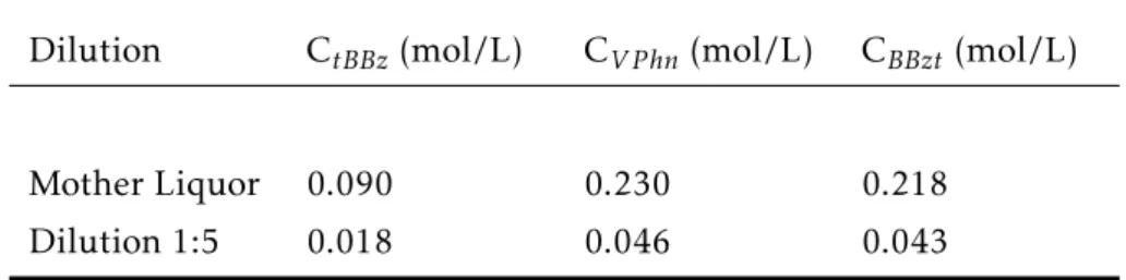
For the single components, two solutions were prepared, one close to the saturation concentration, and the other a dilution of 1:5 of the first for each component. Two 10-step gradient Frontal Analysis for each component and each solution were performed in a HPLC system, which was programmed to increase the inlet concentration by 10% of the solution concentration each 7 minutes, starting at 10% and ending at 100%. The flow rate was 2 ml/min, with a total experiment time of 91 minutes, including elution. For those experiments, the outlet had to be collected in fractions, two per minute, because BBzt had a significant amount of impurities, so only the fractionation could give the pure BC for BBzt. For the other components, fraction collection was performed as well for the experimental protocol to be consistent. The fraction collector is a part of Dionex Ultimate 3000 series and also produced by Thermo Scientific. The prepared solutions are shown below:

Table 3.2: Solutions Concentrations for Single Components

Dilution C_tBBz(mol/L) C_{V Phn}(mol/L) C_BBzt (mol/L)

Mother Liquor 0.090 0.230 0.218

Dilution 1:5 0.018 0.046 0.043

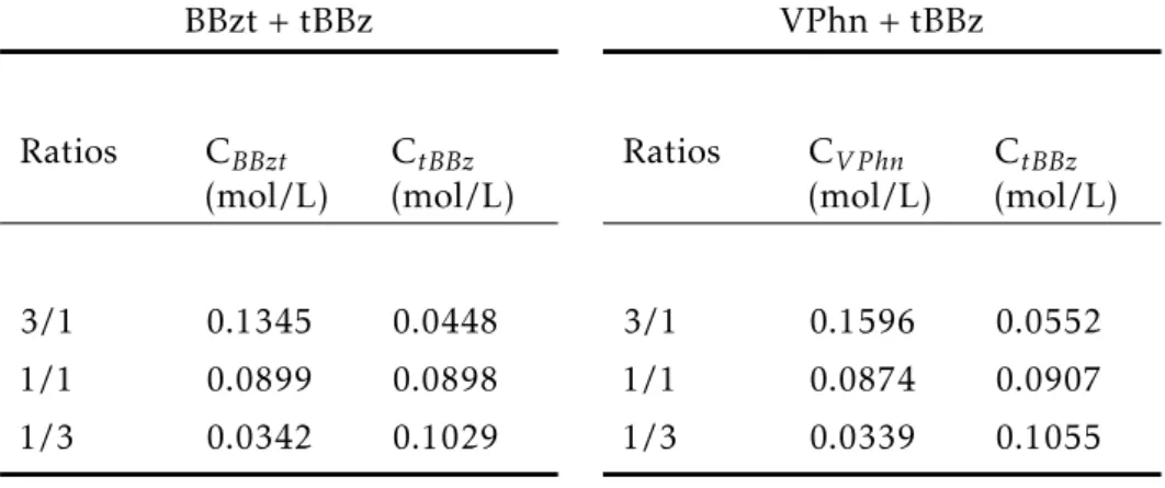
For each mixture, three solutions were prepared. The components in each solution were mixed according to a molar ratio of 1/1, 1/3 and 3/1, close to the saturation concen-tration, with the numerator representing VPhn or BBzt and the denominator tBBz. For

(41)

each ratio, three frontal analysis were made with 33, 67 and 100% of the mother liquor. In each frontal analysis the outlet was fractionated, one fraction each 0.15 minutes, in a total of 93 fractions. The flow rate was 2 ml/min and the injection time was 7 minutes, with a total experiment time of 25 minutes, including elution. Below it is shown a table with the prepared solutions:

Table 3.3: Concentrations used for Binary Mixtures

BBzt + tBBz

Ratios C_BBzt (mol/L)

C_tBBz (mol/L)

3/1 0.1345 0.0448 1/1 0.0899 0.0898 1/3 0.0342 0.1029

VPhn + tBBz

Ratios C_{V Phn} (mol/L)

C_tBBz (mol/L)

3/1 0.1596 0.0552 1/1 0.0874 0.0907 1/3 0.0339 0.1055

To determine the saturation concentrations, solubility tests were performed. These solubility tests were a rough way to determine the range of concentrations that could be used for the determination of the isotherm parameters. The components were weighted in a mass flask respecting the molar ratios as good as possible and then it was added solvent until the solution turned homogeneous.

Regarding the analysis of all the samples collected for every experiment, the HPLC auto-sampler was used. For single components, the injection volume was 1µl, the analysis time per sample was 2.5 minutes with a flow rate of 3 ml/min. For mixtures, the injection volume was 1 µl, the analysis time per sample was 2.5 minutes and the flow rate was 3 ml/min. For every analysis of every sample, the injection was always repeated twice, to check for reproducibility. UV signal was used for component detection. For single components the wavelengths used were 260, 280, 330 and 360 nm and for mixtures 215, 230, 254 and 280 nm.

(42)

C H A P T E R 3 . E X P E R I M E N TA L P R O TO CO L

inlet concentrations for every experiment, a function can be fitted to those data. In this work, the third order polynomial function passing through the origin (when x0 term doesn’t exist) and the power function were used for single components and mixtures, respectively. The fitting was performed with the help of the MatLab software, using the

lsqcurvefit function. This function uses the Least Squares algorithm for curve fitting.

(43)

C

h

a

p

t

e

r

4 Da ta A n a ly s i s

As said in section 3, the components were chosen for having similar molecular sizes but diff_{erent functional groups. The molecular forms are:}

(a) Valerophenone (b) Butyl Benzoate (c) tert-Butylbenzene

Figure 4.1: Molecular Structure of the three components used

4.1 Pure Components Isotherms

(44)

C H A P T E R 4 . DATA A N A LYS I S

4.1.1 Valerophenone

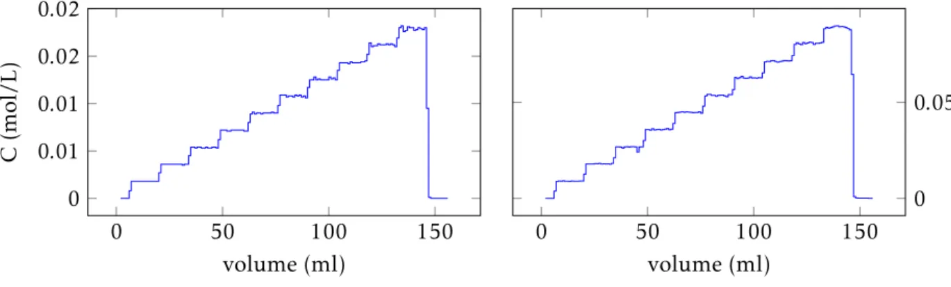
Below the two profiles obtained are presented:

0 50 100 150

0 0.02 0.04

volume (ml)

C

(mol/L)

0 50 100 150

0 0.1 0.2

volume (ml) Figure 4.2: Valerophenone Raw Data

These plots represent the chromatograms obtained using the softwareChromeleon

after converting the absorbance units for molar concentrations, so each plateau repre-sents a percentage of the mother liquor’s concentration. The next step is to calculate the accumulated moles in the column.

The approach used was to divide the data in injection times: since the injection time was 7 minutes or an injection volume of 14 ml because the flow rate was 2 ml/min, and the first injection was at 2 ml, the first BC is from 2 to 16 ml, the second from 16 to 30 and so on until the last step is reached.

The next step is to calculate the accumulated moles of each BC. For that, numerical methods have to be used, and in this work it was used the trapezoids method with the help of MatLab. It was also used the equal area method explained in section 2.1. To better demonstrate the calculation method let’s assume that, since the concentrations of the mother liquors are known, the concentration of each plateau can be expressed in this form:

Ci=j.C0 (4.1)

Wherei= 1, ...,number of plateaus andj= 0.1,0.2, ...,1 represents the mother liquor fractionation for each step.

Now that the concentrations are known, it’s possible to calculate the equal area volume with this expression:

(InjV oli+1−EqualV oli)(Ci−Ci−1) =

Z InjV ol_i₊₁ InjV oli

BC(V)dV (4.2)

With this expression being valid only from the second BC onwards. For the first BC the

Ci−1is 0. After obtaining this value, it’s easy to calculate the accumulated moles in that injection:

(45)

4 . 1 . P U R E COM P O N E N T S I S O T H E R M S

Macc,p,i= (Ci−Ci−1)(EqualV oli−InjV oli−V0,sys) (4.3)

Being, again, valid only from the second BC onwards. the indexpmeans partial accumu-lated moles, the accumuaccumu-lated moles in each injection increase.

Since, until now, this process only calculates the accumulated moles in each step increase, not the actual accumulated moles inside the column, the way to do that is to add the accumulated moles of the previous steps, so:

Macc,1=Macc,p,i

Macc,i= i X

k=1

Macc,p,k

(4.4)

The accumulated moles inside the column calculated represent the moles in the bulk liquid that are always inside the column and the moles adsorbed in the stationary phase. Knowing this, it’s easy to calculate the molar concentration of solute in the adsorbent the following way:

qi=

Macc,i−Ci.V0

Vs

(4.5) This process was applied in both experiments referred, and now, since the adsorbed moles calculated are specific for each concentration, the data can be agglomerated in a single plot to see the entire isotherm data1:

0 0.05 0.1 0.15 0.2 0.25 0

0.2 0.4 0.6

C (mol/l)

q0

(mol/l)

Figure 4.3: Valerophenone Isotherm Data

(46)

there are three points available for calculation, the lower, average and higher values, so it’s possible to calculate the isotherm data with those data and obtain the error bars showed in Figure 4.3. The sizes of the error bars show that the reproducibility of the analysis was very good.

4.1.2 Butyl Benzoate

For Butyl Benzoate, the chromatograms already converted to molar concentrations are as followed:

0 50 100 150

0 0.02 0.04

volume (ml)

C

(mol/L)

0 50 100 150

0 0.1 0.2

volume (ml) Figure 4.4: Butyl Benzoate Raw Data

After proceeding the same way as for Valerophenone, the final isotherm data is pre-sented:

0 0.05 0.1 0.15 0.2

0 0.2 0.4 0.6

C (mol/l)

q0

(mol/l)

Figure 4.5: Butyl Benzoate Isotherm Data

1_{the calculation method was applied to all the components, so the next sections will have only the final} data

(47)

Again, the error bars show that a good reproducibility was achieved.

4.1.3 tert-Butylbenzene

For tert-Butylbenzene, everything was made the same way:

0 50 100 150

0 0.01 0.01 0.02 0.02

volume (ml)

C

(mol/L)

0 50 100 150

0 0.05

volume (ml) Figure 4.6: tert-Butylbenzene Raw Data

Which can be determined the following isotherm data:

0 0.01 0.02 0.03 0.04 0.05 0.06 0.07 0.08 0.09 0

0.2 0.4 0.6

C (mol/l)

q0

(mol/l)

Figure 4.7: tert-Butylbenzene isotherm data

(48)

4.1.4 Parameter Estimation

Now that the isotherm data is determined, the last thing to do is to fit an isotherm model to obtain the isotherm parameters. To reach that objective, the MLMC derivation with a finite number of layers was used. Because the goal is to compare these parame-ters to those of the multi components, the single components were fitted two at a time, VPhn with tBBz and BBzt with tBBz to match with the mixtures’ components. Since all components have identical molecular size (they are all benzene derivatives), the MLMC model assumes thatqMAX andnare constant, so the three components should be fitted altogether. However, if the fittings are done separately, it’s possible to compare the same parameters and see if they are identical or not. That being sad, the problem has to be divided in two objective functions to be minimized. Fori=BBzt, tBBz the objective func-tion is:

ObjFun_BBzt,tBBz=X

i 20 X

j=1

q_calc,i,j−q_exp,i,j2 (4.6)

And fori=VPhn, tBBz:

ObjFunV Phn,tBBz=

X i 20 X j=1

qcalc,i,j−qexp,i,j 2

(4.7)

For solving this minimization problem, again MatLab was used. The function used wasfmincon, which deals with constrained non-linear minimization. The algorithm used was the Active Set Algorithm. A good explanation for this algorithm can be found on-line in the MatLab documentation [22].

For each minimization problem, the parameters to be adjusted areqMAX, nandK1 andK2for each component, with a total of six parameters. The only constraint used was that all parameters have to be greater than or equal to zero. The next figure shows the fitting results for BBzt and tBBz:

(49)

0 0.02 0.04 0.06 0.08 0.1 0.12 0.14 0.16 0.18 0.2 0.22 0

0.1 0.2 0.3 0.4 0.5 0.6 0.7 0.8

C (mol/l)

q

(mol/l)

BBzt exp BBzt fit tBBz exp

tBBz fit

Figure 4.8: MLMC Model fitted for BBzt and tBBz

And for VPhn and tBBz:

−₀_._{02 0} ₀_._{02 0}_._{04 0}_._{06 0}_._{08 0}_._{1 0}_._{12 0}_._{14 0}_._{16 0}_._{18 0}_._{2 0}_._{22 0}_._{24 0}_.₂₆ 0

0.1 0.2 0.3 0.4 0.5 0.6 0.7

C (mol/l)

q

(mol/l)

VPhn exp VPhn fit tBBz exp tBBz fit

(50)

The estimated parameters for both fittings can be shown in the table below: Table 4.1: Estimated parameters for each fitting

VPhn and tBBz

Constants VPhn tBBz

K1 0.568 3.096

K2 10.245 5.602

q_MAX 2.352

n 2.647

ObjFun 8.799×₁₀−4

BBzt and tBBz

Constants BBzt tBBz

K1 1.117 3.413

K2 1.314 4.672

q_MAX 2.192

n 9.998

ObjFun 2.124×₁₀−4

By having two objective functions that share some parameters, like K1 and K2 of tBBz, n and q_MAX, it would be expected that those parameters would be equal, or at least identical. When it comes to q_MAX, the values are quite close, which means that the model’s assumption that q_MAXis always the same if the molecules have identical size and the stationary phase remains the same is not violated. Regarding K1and K2of tBBz, the values are somewhat close to each other, which was expected. The number of layers should be the same for both fittings but it is not. The diff_{erence is quite big because above} 10, the number of layers doesn’t change much, so it can be considered infinite. Since this work is based on RPLC, the stationary phase is hydrophobic, so the less polar the solutes are, the bigger the affi_{nity with the adsorbent. Saying that, and looking at Figure 4.1, the} molecules will bind with the carbon chain (an alkane), the least polar site [20]. As stated in [20], ketones are more polar than esters or alkenes, so probably VPhn, after binding in the surface with the butane chain, acts as a terminator, since the part that’s not bidden is polar, which explains the reduced number of layers compared with BBzt and tBBz.

(51)

4.2 Multi-Component Isotherms

In this section, the raw data of the mixtures were analysed. In this case, the calculation method was diff_{erent because it was performed only single step FA for each mixture and} each ratio. A good example for a single step FA is shown in Figure 1.3. In terms of calculation the equal area method was used, but now, since each experiment had an elution part, the accumulated moles could be calculated in two diff_{erent ways, so the} further fitting of the isotherm data could be more precise.

In Figure 1.3 there is a loading and an elution part. It’s seen two inflection points in which it’s possible to obtain two equal area volumes.

As explained earlier in section 3.2 the value range used to calculate the plateaus for all BC of mixtures was from 10 to 15 ml. Using these values, equal area volumes were determined, but first it’s needed to calculate the inlet concentrations for each mixture and each ratio. Assuming that there arei= 1,2 mixtures,j = 1,2,3 ratios,k= 1,2 components and beingf = 0.33,0.67,1 the inlet fractionation for each ratio, described in section 3.2, then the inlet concentrations for each mixture, ratio and component are:

Ci,j,k,f =f .C0,i,j,k (4.8)

And the equal area volumes are:

(15−_{EqV ol}_load,i,j,k,f₎_C_i,j,k,f ₌ Z 15

2+V0,sys

BCi,j,k,f(V)dV

(EqV olelut,i,j,k,f −10)Ci,j,k,f = Z V_end

10

BCi,j,k,f(V)dV

(4.9)

With the subscriptsload andelutmeaning loading and elution, respectively. After this, is quite easy to calculate the accumulated moles in each part of the BC:

Maccload,i,j,k,f = (EqV olload,i,j,k,f −2−V0,sys)Ci,j,k,f

Maccelut,i,j,k,f = (EqV olelut,i,j,k,f −16−V0,sys)Ci,j,k,f

(4.10)

(52)

q_load,i,j,k,f =Maccload,i,j,k,f −Ci,j,k,f

Vads

qelut,i,j,k,f =

Macc_elut,i,j,k,f −_C_i,j,k,f

Vads

(4.11)

These two adsorbed moles should be the same. However, since every experimental work has some experimental error, it’s not quite the same, although really close.

(53)

4.2.1 Butyl Benzoate and tert-Butylbenzene

In here it’s presented the raw data already converted for molar concentrations.

0 2 4 6 8 10 12 14 16 18 20 22 24 26 28 30 32 0

0.02 0.04 0.06 0.08 0.1

volume (ml)

C

(mol/l)

C_BBzt 33% C_BBzt 67% C_BBzt100%

0 2 4 6 8 10 12 14 16 18 20 22 24 26 28 30 32 0

0.02 0.04 0.06 0.08 0.1

volume (ml)

C

(mol/l)

C_tBBz33% C_tBBz67% C_tBBz100%

(54)

0 2 4 6 8 10 12 14 16 18 20 22 24 26 28 30 32 0

0.01 0.01 0.02 0.02 0.03 0.03 0.04

volume (ml)

C

(mol/l)

0 2 4 6 8 10 12 14 16 18 20 22 24 26 28 30 32 0

0.02 0.04 0.06 0.08 0.1

volume (ml)

C

(mol/l)

Figure 4.11: BCs for BBzt and tBBz with 1/3 Ratio

(55)

0 2 4 6 8 10 12 14 16 18 20 22 24 26 28 30 32 0

0.02 0.04 0.06 0.08 0.1 0.12 0.14

volume (ml)

C

(mol/l)

0 2 4 6 8 10 12 14 16 18 20 22 24 26 28 30 32 0

0.01 0.02 0.03 0.04

volume (ml)

C

(mol/l)

Figure 4.12: BCs for BBzt and tBBz with 3/1 Ratio

(56)

Now, the only thing left is to determine the isotherm data, calculated as explained above and presented below:

0.04 0.06 0.08 0.1

0.2 0.3

q0

(mol/l)

BBzt

0.04 0.06 0.08

0.2 0.4 0.6 tBBz

0.01 0.015 0.02 0.025 0.03 0.035 0.05

0.1

q0

(mol/l)

0.04 0.06 0.08 0.1 0.2 0.4 0.6 0.8

0.04 0.06 0.08 0.1 0.12 0.14 0.1

0.2 0.3 0.4

C (mol/l)

q0

(mol/l)

0.02 0.03 0.04

0.1 0.2 0.3

C (mol/l)

Figure 4.13: Isotherm data for BBzt and tBBz. Each row represents 1/1, 1/3 and 3/1 ratios, respectively.

The error bars were calculated the same way as in section 4.1.

(57)

4.2.2 Valerophenone and tert-Butylbenzene

For this mixture, all calculation procedures were the same. Below it’s shown the raw data already converted for molar concentrations.

0 2 4 6 8 10 12 14 16 18 20 22 24 26 28 30 32 0

0.02 0.04 0.06 0.08

volume (ml)

C

(mol/l)

C_{V Phn}33% C_{V Phn}67% C_{V Phn}100%

0 2 4 6 8 10 12 14 16 18 20 22 24 26 28 30 32 0

0.02 0.04 0.06 0.08 0.1

volume (ml)

C

(mol/l)

(58)

0 2 4 6 8 10 12 14 16 18 20 22 24 26 28 30 32 0

0.01 0.01 0.02 0.02 0.03 0.03 0.04

volume (ml)

C

(mol/l)

0 2 4 6 8 10 12 14 16 18 20 22 24 26 28 30 32 0

0.02 0.04 0.06 0.08 0.1

volume (ml)

C

(mol/l)

Figure 4.15: BCs for VPhn and tBBz with 1/3 Ratio

(59)

0 2 4 6 8 10 12 14 16 18 20 22 24 26 28 30 32 0

0.02 0.04 0.06 0.08 0.1 0.12 0.14 0.16 0.18

volume (ml)

C

(mol/l)

0 2 4 6 8 10 12 14 16 18 20 22 24 26 28 30 32 0

0.01 0.02 0.03 0.04 0.05 0.06

volume (ml)

C

(mol/l)

(60)

Again, with this data is easy to calculate the isotherm data, presented below:

0.04 0.06 0.08 0.05

0.1 0.15 0.2 0.25

q0

(mol/l)

VPhn

0.04 0.06 0.08

0.2 0.4 0.6 tBBz

0.01 0.015 0.02 0.025 0.03 0.035 0.02

0.04 0.06 0.08

q0

(mol/l)

0.04 0.06 0.08 0.1 0.2 0.4 0.6 0.8

0.06 0.08 0.1 0.12 0.14 0.16 0.1

0.2 0.3 0.4

C (mol/l)

q0

(mol/l)

0.02 0.03 0.04 0.05

0.2 0.3

C (mol/l)

Figure 4.17: Isotherm data for VPhn and tBBz. Each row represents 1/1, 1/3 and 3/1 ratios, respectively.

4.2.3 Parameter Estimation

To estimate the model parameters in the mixtures data, MatLab and the same algo-rithm for the single components were used. Each mixture data was fitted separately so later the parameters could be compared and analysed. Considering the reasons stated, two objective functions were used:

ObjFuni=

X

j X

k

qcalc,i,j,k−qi,j,k 2

(4.12)

(61)

Withi,j andkbeing the mixtures, ratios and components, respectively.

Again,qMAX andnare assumed constant in each mixture and adding K1and K2of each component, there’s a total of 6 parameters for each minimization problem. After fitting, the results can be seen below:

0.04 0.06 0.08 0.1

0.2 0.3

q0

(mol/l)

BBzt BBzt exp

BBzt fit

0.04 0.06 0.08

0.2 0.4 0.6 tBBz

tBBz exp tBBz fit

0.01 0.015 0.02 0.025 0.03 0.035 0.04

0.06 0.08 0.1 0.12

q0

(mol/l)

BBzt exp BBzt fit

0.04 0.06 0.08 0.1 0.2 0.4 0.6 0.8 tBBz exp

tBBz fit

0.04 0.06 0.08 0.1 0.12 0.14 0.1

0.2 0.3 0.4

C (mol/l)

q0

(mol/l)

BBzt exp BBzt fit

0.02 0.03 0.04

0.1 0.2 0.3

C (mol/l) tBBz exp

tBBz fit

(62)

0.04 0.06 0.08 0.05

0.1 0.15 0.2

q0

(mol/l)

VPhn VPhn exp

VPhn fit

0.04 0.06 0.08

0.2 0.4 0.6 tBBz

tBBz exp tBBz fit

0.01 0.015 0.02 0.025 0.03 0.035 0.02

0.04 0.06 0.08

q0

(mol/l)

VPhn exp VPhn fit

0.04 0.06 0.08 0.1 0.2 0.4 0.6 0.8 tBBz exp

tBBz fit

0.06 0.08 0.1 0.12 0.14 0.16 0.1

0.2 0.3 0.4

C (mol/l)

q0

(mol/l)

VPhn exp VPhn fit

0.02 0.03 0.04 0.05 0.1 0.2 0.3 0.4

C (mol/l) tBBz exp

tBBz fit

Figure 4.19: Fitted model for VPhn and tBBz. Each row represents 1/1, 1/3 and 3/1 ratios, respectively.

(63)

4 . 3 . E X P E R I M E N TA L VA L I DAT I O N

In this table, the parameter’s values can be seen:

Table 4.2: Estimated parameters for each mixture

VPhn + tBBz

Constants VPhn tBBz

K1 1.866 9.782

K₂ 5.539 11.352

q_MAX 0.661

n 21.405

ObjFun 0.0175

BBzt + tBBz

Constants BBzt tBBz

K1 2.58 9.115

K₂ 6.068 10.829

q_MAX 0.736

n 10.195

ObjFun 0.0134

By looking at these data, the values ofn, as explained above, have practically the same influence, the K1and K2values for tBBz are pretty close, as well as the qMAXvalues.

4.3 Experimental Validation

To determine the isotherm data for single components two 10-step FA analysis were performed. In this work fraction collection had to be used because of impurities in BBzt, but usually it is not needed, only UV signal is required. Meanwhile, the experimental work for mixtures is much more complex: fraction collection is inevitable and to obtain good data, several ratios with several FA per ratio have to be performed and further fraction analysis has to be made, which consumes lots of time and resources, being very prone to human errors too. It would be good if the MLMC model could describe the isotherm behaviour for mixtures with only experimental data for the single components. In this section, cross-check of the parameters for single and multi-component systems will be presented, to see if the isotherms are well predicted with only the single component data.

(64)

0.04 0.06 0.08 0.1

0.2 0.3 0.4

q0

(mol/l)

VPhn VPhn exp

VPhn fit

0.04 0.06 0.08

0.2 0.4 0.6 tBBz

tBBz exp tBBz fit

0.01 0.015 0.02 0.025 0.03 0.035 0.05

0.1 0.15

q0

(mol/l)

VPhn exp VPhn fit

0.04 0.06 0.08 0.1 0.2 0.4 0.6 0.8 tBBz exp

tBBz fit

0.06 0.08 0.1 0.12 0.14 0.16 0.2

0.4 0.6

C (mol/l)

q0

(mol/l)

VPhn exp VPhn fit

0.02 0.03 0.04 0.05 0.1 0.2 0.3 0.4

C (mol/l) tBBz exp

tBBz fit

Figure 4.20: Cross-check for VPhn and tBBz. Each row represents 1/1, 1/3 and 3/1 ratios, respectively.

For this multi component system, the correlation coeffi_{cient (R}2_{) was 0.937. As seen,} the single component parameters fit tBBz data very well but not VPhn data. For this component, more mixture data should be included in the fitting to obtain better behaviour descriptions.

(65)

0.04 0.06 0.08 0.1

0.2 0.3

q0

(mol/l)

BBzt BBzt exp

BBzt fit

0.04 0.06 0.08

0.2 0.4 0.6 tBBz

tBBz exp tBBz fit

0.01 0.015 0.02 0.025 0.03 0.035 0.05

0.1

q0

(mol/l)

BBzt exp BBzt fit

0.04 0.06 0.08 0.1 0.2 0.4 0.6 0.8 tBBz exp

tBBz fit

0.04 0.06 0.08 0.1 0.12 0.14 0.1

0.2 0.3 0.4

C (mol/l)

q0

(mol/l)

BBzt exp BBzt fit

0.02 0.03 0.04

0.1 0.2 0.3

C (mol/l) tBBz exp

tBBz fit

Figure 4.21: Cross-check for BBzt and tBBz. Each row represents 1/1, 1/3 and 3/1 ratios, respectively.

(66)

After using the single component parameters in the multi component systems, now it’ll be presented the inverse, multi component parameters in the single component sys-tems:

−₀_._{02 0} ₀_._{02 0}_._{04 0}_._{06 0}_._{08 0}_._{1 0}_._{12 0}_._{14 0}_._{16 0}_._{18 0}_._{2 0}_._{22 0}_._{24 0}_.₂₆ 0

0.1 0.2 0.3 0.4 0.5 0.6 0.7

C (mol/l)

q

(mol/l)

VPhn exp VPhn fit tBBz exp tBBz fit

Figure 4.22: Cross-check for VPhn and tBBz

For VPhn and tBBz, the fitting is not bad in total, although for VPhn the tendency is not a good match. In the data it’s detected a little curvature, suggesting an s-shape and the predicted data show a too accentuated anti-langmuirian curvature. For tBBz, the fitting is quite good. The slope is not the same, but the tendency quite matches and in low concentrations the fitting is quite good. The global R2for this cross check was 0.941.

(67)

0 0.02 0.04 0.06 0.08 0.1 0.12 0.14 0.16 0.18 0.2 0.22 0

0.1 0.2 0.3 0.4 0.5 0.6 0.7

C (mol/l)

q

(mol/l)

BBzt exp BBzt fit tBBz exp

tBBz fit

Figure 4.23: Cross-check for BBzt and tBBz

(68)

(69)

C

h

a

p

t

e

r

5

C o n c l u s i o n s

In overall, the results of this work were quite successful.

The MLMC model could be fitted in both single and multi component systems sep-arately. However, when parameters were compared and analysed, some big deviations were noticed, particularly in the number of layers. These deviations have logical expla-nations, but more experimental data is needed to be certain of these theories. When trying to study the predictability of multi component isotherm behaviours with single component parameters, it was quite good, for BBzt and tBBz but not for VPhn. Probably some unknown behaviour occurs when VPhn and tBBz are mixed.

When it comes to the cross check data, it was quite successful for tBBz and BBzt, but not that much for VPhn. One solution is to obtain more data from the multi component system, more concentration points for each ratio and more ratios, which is not practical at all, especially because the experimental work required is quite extensive, complex and consumes lots of time and resources. Another solution is to try and analyse single component data with some mixture data and fit altogether. Mixing multi component with single component data could give a better prediction of the mixture isotherms and help to reduce experimental work.

(70)

(71)

B i b l i o g r a p h y

[1] K. K. H. Choy, J. F. Porter, and G. McKay. “Langmuir Isotherm Models Applied to the Multicomponent Sorption of Acid Dyes from Effl_{uent onto Activated Carbon”.} In: (2000).

[2] J. C. Crlttenden, P. Luft, D. W. Hand, J. L. Oravltz, S. W. Loper, and M. Ari. “Pre-diction of Multicomponent Adsorption Equilibria Using Ideal Adsorbed Solution Theory”. In: (1985).

[3] A. Erto, A. Lancia, and D. Musmarra. “A modelling analysis of PCE/TCE mix-ture adsorption based on Ideal Adsorbed Solution Theory”. In: Separation and Purification Technology(2011).

[4] T. Fornstedt, P. Forssen, and J. Samuelsson. “Modeling of Preparative Liquid Chro-matography”. In: LIQUID CHROMATOGRAPHY - Fundamentals and Instrumenta-tion(2013).

[5] P. Forssén, R. Arnell, and T. Fornstedt. “A quest for the optimal additive in chiral preparative chromatography”. In: (2009).

[6] F. Gritti, W. Piatkowski, and G. Guiochon. “Comparison of the adsorption equi-librium of a few low-molecular mass compounds on a monolithic and a packed column in reversed-phase liquid chromatography”. In: (2002).

[7] G. Guiochon, S. G. Shirazi, and A. M. Katti. Fundamentals of Preparative and Non-linear Chromatography. 1994.

[8] P. Jandera. “LIQUID CHROMATOGRAPHY - Normal-Phase”. In: (2013).

[9] A. Kurniawan, H. Sutiono, N. Indraswati, and S. Ismadji. “Removal of basic dyes in binary system by adsorption using rarasaponin–bentonite: Revisited of extended Langmuir model”. In: (2012).

[10] J. W. Lee and A. Seidel-Morgenstern. “Multi-Layer Multi-Component Langmuir Isotherm Model: A Novel Generic Isotherm Model for Liquid Chromatography”. In:Fundamentals of Adsorption. USA, 2016.