Repositório ISCTE-IUL
Deposited in Repositório ISCTE-IUL: 2020-07-09
Deposited version: Post-print
Peer-review status of attached file: Peer-reviewed
Citation for published item:
Isidro, H. & Dias, J. G. (2017). Earnings quality and the heterogeneous relation between earnings and stock returns. Review of Quantitative Finance and Accounting. 49 (4), 1143-1165
Further information on publisher's website: 10.1007/s11156-017-0619-z
Publisher's copyright statement:
This is the peer reviewed version of the following article: Isidro, H. & Dias, J. G. (2017). Earnings quality and the heterogeneous relation between earnings and stock returns. Review of Quantitative Finance and Accounting. 49 (4), 1143-1165, which has been published in final form at
https://dx.doi.org/10.1007/s11156-017-0619-z. This article may be used for non-commercial purposes in accordance with the Publisher's Terms and Conditions for self-archiving.
Use policy
Creative Commons CC BY 4.0
The full-text may be used and/or reproduced, and given to third parties in any format or medium, without prior permission or charge, for personal research or study, educational, or not-for-profit purposes provided that:
• a full bibliographic reference is made to the original source • a link is made to the metadata record in the Repository • the full-text is not changed in any way
The full-text must not be sold in any format or medium without the formal permission of the copyright holders.
Earnings quality and the heterogeneous relation between earnings and stock returns
Earnings quality and the heterogeneous relation between earnings and stock returns
Abstract
We adopt a heterogeneous regime switching method to examine the informativeness of accounting earnings for stock returns. We identify two distinct time-series regimes in terms of the relation between earnings and returns. In the low volatility regime (typical of bull markets), earnings are moderately informative for stock returns. But in high volatility market conditions (typical of financial crisis), earnings are strongly related to returns. Our evidence suggests that earnings are more informative to investors when uncertainty and risk is high which is consistent with the idea that during market downturns investors rely more on fundamental information about the firm. Next, we identify groups of firms that follow similar regime dynamics. We show that firms with poorer accrual quality have a greater probability of belonging to the high volatility regime.
Keywords: return volatility, accruals, stock market, Markov-switching model, financial crisis JEL classification: G14, M40, M44
1. Introduction
Accounting and finance have a long tradition of studying the relation between accounting earnings and stock market returns. This interest is driven by the importance of earnings for investment decisions and for the prediction of returns. In their asset allocation decisions, investors form expectations about the firm’s future cash flows and the risk associated with these cash flows (Fama et al. 1970). As earnings contain information about the stream of cash flows, investors use earnings information to revise their expectations about cash flows and this leads to a revision of stock prices. In other words, earnings are useful for stock price formation. Prior studies have focused on explaining the time series variation or the sectional variation in the earnings-return relation. We propose to study both the temporal and cross-sectional variation in the relation between earnings, earnings changes and returns using an extension of the regime switching methodology introduced by Hamilton (1989): the heterogeneous regime switching methodology. The heterogeneous regime switching method can be summarized as follows. First we estimate the time series variation in the earnings-returns relation for the sample firms for the period 1997 to 2010. The estimation method allows us to identify breaks in the time series of earnings-returns and to characterize each regime. As a result, we are able to let the data generating process determine the regime rather than identifying the breaks ex-ante which would be subjective. Second each firm is assigned to a group (or cluster) based on how long it stays in one regime and the likelihood of switching to the other regime. Thus the model is dynamic as it allows firms to switch between regimes across time. The periods of stay and the likelihood of switching characterize the regime dynamics.
We identify two regimes. The low volatility regime corresponds to periods of low return volatility and a moderate association between earnings and returns. Both earnings and earnings changes are positively associated with returns but the magnitude of the earnings coefficients is smaller than in the other regime. The high volatility regime represents periods of high volatility in returns with earnings and
earnings changes strongly associated with returns. This result is consistent with the idea that in periods of high price instability, such as financial crises, information about earnings is more important to investors than in “normal” periods. During bear market conditions, investors become more risk averse and fly from stocks with high levels of uncertainty about fundamental value (Vayanos 2004, Lang and Maffett 2011). As financial information lessens uncertainty about the firm’s fundamental value and reduces risk perception, earnings become more important for investors (Leung et al. 2014, Lang and Maffett 2011). In other words, investors rely more on earnings information during market downturns because other information is more likely to reflect speculation and noise.
Next we identify the firms with similar regime dynamics, i.e. firms that spend similar time in each regime and have a similar probability of switching. We find two clusters of firms. Firms in the first cluster have a stable dynamics, i.e. they start and remain in the low volatility regime throughout most of the sample period. Conversely, firms in the second cluster spend more time in the high volatility regime and also have a higher probability of transition to the other regime. We then investigate the properties of accounting information in the two groups of firms. Our aim is to explore whether the quality of financial information, and of other firm fundamentals, is associated with the firms’ regime dynamics. We find that firms with a greater likelihood of being in the high volatility regime (firms in cluster two) have poorer information quality, measured in terms of accrual quality and smoothness. During market downturns, earnings are more unstable due to unexpected losses, impairments, and other unusual transactions. The volatility between earnings and cash flows increases, resulting in poor accrual quality. Regarding other firm-specific characteristics, we find that smaller firms, firms with poor performance, lower market-to-book ratio, and growing firms are more likely to be in the high volatility returns-earnings regime.
We believe that our study contributes to the accounting and finance literature in two ways. First, we demonstrate that a full understanding of the returns-earnings relation entails consideration of both the
time-series variation and cross-sectional variation in this relation. Second, we establish an association between firms’ fundamental characteristics such as accrual quality, and the time and cross-sectional variation in the usefulness of earnings for returns.
The remainder of the paper is organized as follows. Section 2 revises prior literature. Section 3 presents the heterogeneous regime switching model. Section 4 describes the sample and the data, and presents descriptive results. Section 5 reports the estimation results of the heterogeneous regime switching model. Section 6 discusses the link between cluster affiliation and earnings quality. Section 7 concludes.
2. Prior literature
The idea that earnings convey useful information for stock returns has long been established by academics (Ball and Brown 1968; Beaver 1968,Watts and Zimmerman 1986). It relies on three
important theoretical links developed by Watts and Zimmerman (1986) and Beaver (1998). First, current accounting earnings provide information about expected future earnings. Second, current and expected earnings help predict the firm’s stream of future cash flows. Third, stock prices represent the present value of expected future cash flows. The view that earnings are useful to investors has also been endorsed by accounting standard setters around the world. For example, both the FASB (Financial Accounting Standards Board) in the US and the IASB (International Accounting Standard Board) define the primary objective of financial reporting as the provision of information that is useful to capital providers in making decisions about allocating resources to the firm (IASB 2010, FASB 2010). The decision-usefulness criterion that guides the preparation of earnings information makes earnings the
widely accepted measure of firm performance. Consequently, earnings-based valuation models are commonly used by academics, practitioners and investors1.
The seminal work of Ball and Brown (1968) and Easton and Harris (1991) introduced a model that evaluates the information usefulness of earnings for returns. The model explains the
contemporaneous relation between returns and current earnings and changes in earnings. Earnings provide investors with useful information if the earnings variables in the model exhibit a considerable explanatory power with respect to returns.2 The large body of literature examining the contemporaneous relation between earnings and returns shows that earnings contain relevant information for stock returns (e.g. Collins and Kothari 1989, Lipe 1990, Easton et al. 1992, Strong 1993, Lamont 1998, Barth et al. 2013). The literature also documents considerable time variation in the usefulness of earnings, with many studies reporting a decline in usefulness. Lev (1987) is one of the first studies showing that both the slope coefficient estimates and the explanatory power of earnings for stock returns decreased over time. Subsequently, Collins et al. (1997), Lev and Zarowin (1999), and Francis and Schipper (1999) also find evidence of a decline in the usefulness of earnings. Lev and Zarowin (1999) ascribe the apparent decline in earnings informativeness to the failure of the accounting system to recognize business innovation (i.e. R&D investment) in a timely matter. Collins et al. (1997) and Francis and Schipper (1999) find that the decrease in the value relevance of earnings is compensated by the increase in the value relevance of book value and hence conclude that the usefulness of the accounting system as a whole has not declined. However, Brown et al. (1999) argue that scale factors influence this result. After controlling for scale effects they find that in fact the usefulness of earnings has deteriorated over time.
1 For a review of earnings-based models see Penman 2012.
2 In this paper we take the common view that value relevance is a direct measure of the usefulness of earnings for stock
returns (Joos and Lang 1994, Collins et al. 1997, Francis and Schipper 1999, Lev and Zarowin 1999, Barth et al. 2001, Francis et al. 2004). Other ways of assessing the usefulness of earnings include: market reaction to earnings announcements (Ball and Brown 1968, Beaver 1968), correlation between earnings and cash flows (Lev et al. 2010), and reliability of
Studies analyzing more recent periods of time also show a decline in the usefulness of earnings for investors (Ryan and Zarowin 2003, Core et al. 2003, Kothari and Shanken, 2003; Dontoh et al. 2004, and Balachandran and Mohanram 2011). The idea that earnings have lost their usefulness has prompted research on the factors driving the decline. One perspective suggests that the efficiency of information processing of stock prices has changed over time. An increase in return volatility linked to non-informed trading hampers the ability of returns to reflect fundamental earnings information (Dontoh et al. 2004). The other view claims that the problem lies with the loss of quality of accounting earnings, i.e. the loss of ability to reflect future cash flows. Several reasons are given for the decline in earnings quality. First, reported earnings do not reflect the information richness of voluntary corporate disclosures (Lundholm and Myers 2002). Second, the increasing abundance of concurrent disclosures, e.g. conference calls and pro-forma disclosure pre-empts the information content of earnings (Amir and Lev 1996, Collins et al. 2009). Third, complex accounting issues such as fair value measurements and intangible recognition can reduce the association of earnings with sock returns (Lev and Zarowin 1999, Balachandran and
Mohanram 2011, Dechow et al. 2013). Rajgopal and Venkatachalam (2011) provide evidence consistent with the view that earnings have lost quality over time. They show that the increase in stock return volatility in the US is associated with a decline in the quality of earnings, and that association persists through time. The explanation is that poor earnings quality causes noisier earnings leading to dispersion in investors beliefs about the firm future cash flows. At the same time financial analysts resort more to other sources of information because they view earnings as a weak information signal. This in turn generates more volatility as analysts use diverse sources of information and investors follow different analysts. The recent and growing literature on the consequences of the international adoption of IFRS has also raised concerns about the informativeness of IFRS-based earnings for investors (for recent reviews about the information properties of IFRS earnings see Leuz and Wysocki 2015 and Brown
2013). The weak enforcement structures in place in some jurisdictions, the difficult implementation of certain IFRS concepts such as the fair value measurement, and scope for management discretionary choices have been pointed as factors that can impair the usefulness of accounting information for investors.
If problems with the quality of accounting earnings explain the decline in the returns- earnings relation over time, then we should also expect cross-sectional variation in that relation because
accounting quality is a function of the firm’s activities (Dechow et al. 2010). Amir and Lev (1996) and Core et al. (2003) find that earnings are less related with returns in intangible-intensive firms, Frank (2002) report lower value relevance of earnings in high-growth firms, Burgstahler et al. (2006) show that firms with higher book-tax alignment have lower earnings quality. Further, manager incentives also vary across firms leading to differences in the discretion that managers apply in the preparation and disclosure of earnings. For example Kraft et al. (2014) find that managers and other senior officers engage in accrual earnings management before trading on their own stock.
To summarize, variation in the usefulness of earnings for returns across firms reflects differences in underlying fundamental aspects of the business and in the quality of the accounting system to portray current and future performance. Givoly and Hayn (2000) investigate temporal variation in earnings, cash flows and accruals and address this point. They argue that if time variation in earnings follows the same time-trend as the stream of cash flows (which captures fundamental performance that is not affected by the accounting system), then accounting earnings simply reflects changes in fundamental performance and there are no structural changes in the quality of the accounting system over time. Their results do not confirm this hypothesis. They find that the decline in profitability does not result from a decrease in the underlying cash flows of the firm, but derives from changes in the relation between cash flows and earnings. In other words a change in accounting accruals. This finding suggests that the quality of the
accounting system to capture economic change as captured by accruals is important to explain the time variation in the usefulness of earnings for stock returns. Similarly, studies investigating the cross-sectional relative explanatory power of accruals and cash flows (e.g. Livnat and Zarowin 1990, Dechow 1994) show that accruals have information usefulness beyond that of cash flows. In a similar vein Ryan and Zarowin (2003) report that the time series decline in the in the usefulness of earnings is explained by changes the accrual component of earnings. They conclude that the decline is attributable to the quality of accounting not to the change in the economic conditions of the firms. Studies such as Givoly and Hayn (2000) and Ryan and Zarowin (2003) use accounting conservatism to infer about the quality of the accounting system. Other studies rely on other properties of accounting notably the quality of accruals.3
Prior studies investigating the usefulness of earnings for investors typically focus on either inter-temporal or cross-sectional variation, but not both. A common approach is to explain time variation by the inclusion in the returns-earnings model of the firm factors expected ex-ante to affect that variation (Collins et al. 1997, Ryan and Zarowin 2003, Balachandran and Mohanram 2011, Rajgopal and
Venkatachalam 2011). But that approach fails to consider that the time variation in earnings usefulness does not affect all firms equally. Firms might experience some periods when earnings are more
correlated with returns and others when they are less. Further this cross-sectional variation in the usefulness is likely to be associated with firm-specific conditions which are reflected in earnings and other accounting variables. Notably Collins and Kothari (1989) show that earnings usefulness varies through time and across firms. Collins and Kothari (1989) associate the temporal variation with interest rates and the cross-sectional variation with earnings persistence, growth and risk. They deal with these sources of variation by including controls in the returns regressions but they do not formally model the
3 A review of the earnings quality metrics is beyond the scope of our study. See for example Dechow et al. (2010) for an
time and cross-sectional variation. Another approach is to compare the earnings-returns relation across sub-periods as in Strong (2003). However the ex-ante identification of the sub-periods can be subjective, and there is no theoretical or empirical justification for the breaks. The heterogeneous regime switching methodology provides support for the identification of earnings-returns regimes breaks and identify groups of firms with similar regime dynamics.
3. The heterogeneous regime switching model
This study applies a novel framework based on the regime switching model (RSM) introduced by Hamilton (1989) to study the relation between earnings and returns. Regime switching models can be very useful in economic data modeling because they allow for non-linear stationary processes which are typical in economic problems. They have become very popular in economics and finance as they capture breaks (or discontinuities) in the business cycle (e.g. Krolzig 2001, Tan and Mathews 2010) and in the behavior of economic time series. These discontinuities are typical in the time series of returns where periods of low return volatility and high prices are followed by periods of high return volatility and low prices. For this reason regime switching models have been used in finance to characterize stock market cycles (Bekaert and Harvey 1995, Ang and Bekaert 2002, Aktas et al. 2007, Hwang et al. 2007, Zhu and Zhu 2013). The regime-switching approach was also used to model other economic problems. Recent examples include Tang and Change (2015) who uses switching regression model to classify firms into strong and weak governance, and Paeglis and Veeren (2013) who model the speed at which venture capitalists exit a firm after its IPO. Our approach differs from the one adopted in these studies in that we not only estimate the regimes but we also allow for firm heterogeneity. This approach allows us to identify clusters of firms with different regime dynamics. Our model also extends the regime-switching
framework by introducing cluster-level dynamics. Based on the evidence that the returns-earnings relation can be affected by heterogeneity in firm conditions we assume more than one latent Markov process that is characterized by a transition probability between each of the regimes. The HRSM - Heterogeneous Regime-Switching Model (Dias et al. 2008, Ramos et al. 2011) enables the statistical estimation of regime-switching models based on the similarity of the dynamics associated with each homogeneous group of firms (or clusters). A model with 𝑆 clusters is denominated HRSM-S. In other words, we identify distinct groups of firms in terms of returns-earnings relation following Markov chains with distinct probabilities of transition from one regime at time t to another regime at time t+1. Next we explain the HRSM-S model.
Let 𝑅 represent the compounded stock return of firm 𝑖 at quarter 𝑡, where 𝑖 ∈ 1, … , 𝑛 and 𝑡 ∈ 1, … , 𝑇 . Let f R ; ψ be the probability density function associated with the returns for firm i. The HRSM-S (𝑆 being the number of groups or clusters associated with this application) is given by:
f R ; ψ ∑ ∑ ∑ … ∑
f w
i, z
i1, … , z
iTf R
i|w
i, z
i1, … , z
iT (1)The right-hand side of Equation (1) indicates that the underlying model architecture is typical of a mixture model consisting of the time-constant latent variable 𝑤 and 𝑇 realizations of the time-varying latent variable z . In this context, the observed data density f R ; ψ is obtained by marginalizing over the latent variables. Furthermore, the term
𝑓 𝑤 , 𝑧 , … , 𝑧
of Equation (1) can be further transformed into:where 𝑓 𝑤 essentially represents the probability of a given firm belonging to a given latent class or cluster 𝑤 , with multinomial parameter 𝜆 𝑃 𝑊 𝑤 , 𝑓 𝑧 |𝑤 represents the initial-regime probability and f z |z, - , w represents the latent transition probability. Moreover, the observed return
depends only on the regime applicable at that specific time point, i.e., response 𝑅 is independent of returns at other moments (this is known as the local independence assumption). Simultaneously, the said observed return value is also independent of latent states at other times. These assumptions can be formulated as follows:
f R |w , z , … , z ∏ f R |z (3)
where the probability density that a particular observed stock return value at time 𝑡 conditional on the regime in place at that chronological point – f R |z – is assumed to have the specification of a univariate Gaussian density function.
We consider the following regression structure that explains stock returns as a function of earnings and earnings changes (plus industry indicators):
E R |z k, x β β E β ∆E θ IND (4)
𝑅 is the compounded quarterly returns of firm i at quarter t calculated as 𝑙𝑜𝑔 𝑃 /𝑃, and vector x
contains the independent variables (𝐸 , ∆𝐸 , 𝐼𝑁𝐷 , … , 𝐼𝑁𝐷 . 𝐸 isquarterly earnings per share scaled by price at the beginning of the quarter. ∆E is change in quarterly earnings per share from quarter t-1 to quarter t, scaled by price at the beginning of the quarter, and IND is a set of industry indicators based on the one-digit standard industry classification (SIC) industry r and zero otherwise. Industry 3 (industrials
and electronics) is the reference category, thus θ 0. The model is heteroskedastic as the variance of returns depends on the regime: Var R |z k, x σ .
The parameters of the model are estimated using the maximum likelihood method. The Expectation-Maximization (EM) algorithm can subsequently be employed to solve the maximization of the log-likelihood function. Nevertheless, it should be pointed out that the application of the EM algorithm requires both a lengthy computational effort and a cumbersome computer storage capacity. Therefore, the application of this algorithm is often impractical, if not impossible. To circumvent this operational problem, a special variant of the EM algorithm – the Baum-Welch (BM) algorithm – has been advanced by the literature, enabling the above-mentioned maximization problem to be more easily solved (Dias et al. 2008). Furthermore, the choice of the appropriate number of latent classes 𝑆 is traditionally based on the analysis of statistical information criteria. We use the BIC criterion (Schwarz 1978), and we identify the most appropriate value of S when the value of BIC is at its minimum.
4. Sample, data and descriptive results
In the empirical analysis we use quarterly data from 1997 to 2010. The sample comprises US firms from the interception of Compustat and CRSP databases, and with complete financial and return data. As in prior studies, we eliminate cases with negative book values. The final sample includes 2,140 firms with 60 quarters of returns and earnings data.
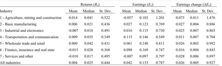
Table 1 presents descriptive statistics for the returns and earnings variables by industry. During the sample period the average (median) compunded stock return is 0.004 (0.025), but there is substantial variation in returns both within and across industry. The agricultural, mining and construction industry has the highest returns, whereas the financial sector exhibits the lowest returns. The average
earnings-to-lagged price ratio is 0.042 but there is also cross-industry and cross-firm heterogeneity. The large standard deviations in returns and earnings suggest that accounting earnings and stock returns (and thus the returns-earnings relation) are affected by firm-specific conditions. We explore how firm specific conditions explain heterogeneity in the returns-earnings relation in section 5.
< Table 1 about here >
Figure 1 plots the time variation in the correlation between returns and earnings, and between returns and changes in earnings. The volatility in the returns-earnings correlation is evident, with periods of high positive correlation followed by periods of low and negative correlation. The three peaks of large negative correlations correspond to important stock market crashes: the 1998-1999 Asian crisis and Russian ruble crisis, the 2002-2003 internet bubble crash, and the most recent financial crisis in 2008-2009. In periods of dramatic decline in stock markets, accounting earnings are more strongly correlated with returns albeit negatively. This is because reliable information about firm fundamentals becomes more important for investors when uncertainty is high and concerns about the firm’s future cash flows are more acute (Lang and Maffett 2011, Lang et al. 2012).
< Figure 1 about here >
5. Results of the estimation of the heterogeneous regime switching model
Table 2 presents the estimation results of the heterogeneous regime switching model. We identify a dual returns-earnings regime characterized by low return volatility and high return volatility. In the low volatility regime, the level of returns is positive and the return variance is relatively low (0.045). In such bull market conditions earnings and earnings changes are moderately useful in explaining returns. That is,
in good times investors are likely to use other sources of information besides information about accounting earnings to make investment decisions (e.g. news from the press and other non-financial information). In contrast, fundamental earnings information becomes more important when uncertainty and volatility are high. The high volatility regime in our model mimics the characteristics of the market in a bear state or in a crash: negative stock returns (represented by the negative intercept) and high return volatility (the variance is 0.435). In this regime the coefficients of earnings and earnings changes are more important in explaining stock returns than in the low volatility regime which implies that earnings information is more useful for investors in depressed stock markets. The negative coefficient of earnings reflects the high prevalence of losses in periods of markets crash and negative stock returns. This result is consistent with prior findings that losses lead to negative earnings response coefficients (Hayn 1995).
Negative shocks to returns lead to large return volatility (French et al. 1987, Schwert 1989, Edwards et al. 2003, Schwert 2011). The large volatility is explained by three phenomena: high uncertainty about the firm’s future cash flows, high risk perception, and general decline in prices and asset liquidity. Fundamental financial information about the business can help attenuate uncertainty and risk perception resulting in investors relying more on earnings information when markets are depressed. Leung et al. (2014) study bank holdings during the recent financial crisis and conclude that banks’ fundamental information, including earnings, was the major criterion used by investors to make investment decisions in the crisis period. Similarly, Lang and Maffett (2011) contend that transparent financial information lessens the uncertainty about the firm’s fundamental value which is particularly pronounced during market downturns. In such periods, financial information becomes more important because of the “flight to quality” behavior where investors become more risk averse and flee from stocks with high levels of uncertainty on fundamental value (Vayanos 2004, Lang and Maffett 2011). This view is also proposed by the Securities and Exchange Committee (SEC). In a speech on the role of accounting in preventing
financial crisis the SEC Chief Accountant concludes “when pressures are highest, and investor confidence has the greatest potential to be shaken by uncertainty, the importance of transparent, objectively audited financial reporting to investors, and an independent and objective system to establish standards for such reporting, are necessary and critical components to both short term and long term success” (SEC, April 2011).
< Table 2 about here >
Next, we describe the dynamics of the two return-earnings regimes across latent classes (Table 3). The BIC criterion indicates there the sample firms can be clustered two groups of firms with distinct dynamics. The groups or clusters are created based on the firm’s similarity in terms of the likelihood of being in each regime and likelihood of switching to the other regime. Firms in cluster one have a large total probability of being in the low volatility regime (the probability of being in the low volatility regime is 0.784 whereas the probability of being in the high volatility regime is only 0.216). Further, firms in cluster one start in a low volatility regime (the initial probability is 0.912) and stay in that regime. The probabilities of transition between regimes are relatively low but distinct between clusters. The transition probability between low and high volatility regimes is almost three times higher in cluster two than in cluster one. On the other hand, the probability of transition from high to low volatility is higher in cluster one than in cluster two. The (mean) sojourn time measures the expected time in quarters that a firm takes to move out of a given regime. Firms in cluster one take 20.6 quarters to move out of the low volatility regime, but take only 6 quarters to move out of the high volatility regime. Firms in cluster two are less sticky to return regimes. They have a larger total probability of being in the high volatility return state and a larger sojourn time in that state.
Table 4 shows the industry classification of firms by cluster. The finance sector is the most represented sector in cluster one (30.9% of cluster one firms) while the industrials & electronics is the most represented sector in cluster two (42.5% of cluster two firms). The majority of firms in industries 2 (basic manufacturing), 4 (transportation & communication), 5 (wholesale trade), 6 (finance) and 7 (services) fall in cluster one in terms of the returns-earnings dynamics. But most firms in industry 1 (agricultural, mining & construction) and industry 3 (industrial & electronics) are classified into cluster two.
< Table 4 about here >
5. The association between firm clustering and earnings quality
This section explores the association between the quality of financial information and firms fundamental characteristics and the cross-sectional heterogeneity in the returns-earnings relation. To that end, we estimate the following probit model where the probability 𝑝 of firm 𝑖 being in cluster two versus being in cluster one is estimated by the probit-link function Φ:
𝑝 Φ 𝛾 𝛾 𝐸𝑎𝑟𝑛𝑖𝑛𝑔𝑠𝑄𝑢𝑎𝑙𝑖𝑡𝑦 𝛾 𝑆𝑖𝑧𝑒 𝛾 𝐿𝑒𝑣𝑒𝑟𝑎𝑔𝑒 𝛾 𝐼𝑛𝑡𝑎𝑛𝑔𝑖𝑏𝑖𝑙𝑖𝑡𝑦
𝛾 𝑂𝑝𝑒𝑟𝑎𝑡𝑖𝑛𝑔𝑃𝑒𝑟𝑓𝑜𝑟𝑚𝑎𝑛𝑐𝑒 𝛾 𝑀𝑎𝑟𝑘𝑒𝑡_𝑡𝑜_𝐵𝑜𝑜𝑘 𝛾 𝑆𝑎𝑙𝑒𝑠𝐺𝑟𝑜𝑤𝑡ℎ . (5)
5.1. Measurement of variables
The variable Cluster takes the value of one if the firm is assigned to cluster two (firms that stay longer in the high volatility regime), and zero if it is assigned to cluster one (firms that stay longer in the low volatility regime). To measure earnings quality we use four measures that rely solely on accounting
numbers.4 We use three measures that capture the properties of accounting accruals: the standard deviation, and the absolute value of the residuals of the Dechow and Dichev's (2002) model, and earnings smoothness. The forth variable is persistence which captures solely the time series variation in earnings. These variables have been extensively used in prior research to capture the quality of earnings and they vary substantially across firms. The measures are defined so that higher values imply lower earnings quality. Next we explain how the measures are calculated.
Accruals. Accruals measures are based on the Dechow and Dichev's (2002) model relating total current accruals (TCA) to lagged, current, and future cash flows from operations (CFO). TCA α α CFO, - α CFO, α CFO, ε, , where TCA is total current accruals measured as the quarterly
change in current assets minus the quarterly change in current liabilities, minus the quarterly change in cash, plus the quarterly change in short-term debt. All variables are scaled by lagged total assets. The first accrual quality measure (AccrualQ1) is the standard deviation of ε over the eight-quarter rolling window, and the second measure (AccrualQ2) is the absolute value of ε .
Persistence is the slope coefficient estimate (β ) from an autoregressive model of order one for quarterly earnings per share (E), i.e. E, β β E, - μ,.
Smoothness is the ratio of firm’s standard deviation of net income before extraordinary items to its standard deviation of cash flows from operations, both scaled by lagged total assets (σNI/σCFO), calculated over eight-quarter rolling windows.
We include in the analysis the following firm fundamentals that are likely to affect firm cluster membership, or put differently are likely to affect the cross-sectional variation in the returns-earnings relation. Size defined as the log of total assets, leverage calculated as the ratio of long-term debt to total assets, intangibility measured as the ratio of intangible assets to total assets, operating performance calculated as the ratio of operating profit to sales, market-to-book ratio defined as the market value of equity to the book value of equity, and sales growth defined as the change in quarterly sales divided by previous quarter sales.5
As the assignment of firms to the clusters is time-invariant, we need to reduce the data to one single observation for each firm. Therefore, we use the firm median for each of the variables.6 We also add industry fixed effects to the model to account for time invariant industry differences in cluster composition.
5.2. Empirical results
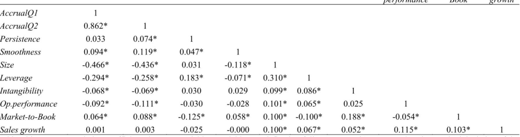
Table 5 reports summary statistics by cluster for the variables used to estimate the probit model. On average, firms in cluster one have higher accrual quality. Firms in this cluster are on average larger, more leveraged, have positive operating profit, and a higher market-to-book ratio. Table 6 presents correlation coefficients. The correlations are generally small. The largest correlations are between accrual variables and size, and between accrual variables and leverage.
5 Another relevant firm fundamental that is not included in the model is cash flow volatility (standard deviation of cash flow
from operation scaled by total assets over the eight quarter window). We do not include it in the tabulated results because Compustat does not report cash flow from operations for several sample firms and thus including the variable would reduce considerably the number of observations. When we re-estimate the model including cash flow volatility we obtain the same results for earnings quality and find that cash flow volatility is higher for cluster 2 firms but only in the persistence and smoothness models.
< Tables 5 and 6 about here >
In Table 7 we present the results of estimating the probability of a firm being assigned to cluster two versus being assigned to cluster one taking into account earnings quality and other firm
fundamentals. The final sample is reduced to 2,128 firms because of missing values for some of the control variables. The most interesting result is the positive association between accruals-based
measures of earnings quality and the probability of the firm following the dynamics of cluster two. The positive and significant coefficient for the accruals measures indicates that firms that are more likely to be in the high volatility regime experience higher volatility in accruals. For AccrualQ1 (AccrualQ2), a unit decrease in accrual quality is associated with an increase in the probability of the firm being assigned to cluster two by 23.5% (14.9%). The result is consistent with prior findings that return volatility and poor quality of accruals are positively associated (Rajgopal and Venkatachalam 2011). One interpretation for the results is that in periods of financial crisis earnings volatility increase due to the recognition of impairment losses, provisions, and other non-recurring transactions. As accruals capture how well accounting earnings map into cash flows, deterioration in the relation between earnings and cash flows causes noisier accruals. We find similar results for smoothness, a measure that also captures the relation between earnings and cash flows. However, we do not find an association between earnings persistence and cluster affiliation. This is not surprising because persistence merely reflects how past earnings predict contemporaneous earnings but it is not informative about the link between earnings and cash flows.
< Table 7 about here >
Regarding other firm specific characteristics, we note that smaller firms, firms with poorer operating performance, lower market-to-book, and larger sales growth, are more likely to follow cluster two dynamics than cluster one dynamics. This profile is characteristic of a young and fast-growing firm.
Younger firms are more likely to experience higher returns-earnings volatility because they are not yet established businesses and there is more uncertainty about their accounting information. Overall the empirical analysis suggests that cross-sectional variation in earnings quality captured by accruals is associated with the likelihood of firms experiencing high volatility in terms of earnings-returns.
6. Conclusion
The degree to which accounting earnings provides useful information for stock markets is of considerable interest to businesses, investors and regulators. Accounting earnings is an important piece of information because it influences investors’ expectations about the firm’s future prospects. A number of academic studies document a decline in the usefulness of earnings for returns and suggest that
increased return volatility and deterioration in the quality of the accounting system explain the decline. We add to that debate by investigating how a firm-level variation in the quality of earnings is related to both the time-series and cross-sectional variation in the returns-earnings relation. Differently from prior research, we adopt a heterogeneous regime switching methodology that allows us to model both the inter-temporal and cross-sectional variation in the relation between earnings and stock returns. This method permits the identification of time-series regimes, and then allocates firms to clusters based on regime dynamics. We identify two distinctive regimes: a low and a high volatility regime. In the low volatility regime, stock returns are positive and stable and earnings moderately explain stock returns. In the high volatility regime, returns are negative and highly volatile (typical of financial crises). In this regime, earnings are strongly associated with returns indicating that earnings information is more important to investors when uncertainty and risk-perception are high. We next identify two distinct groups of firms with different regime-switching dynamics and we show that the dynamics are associated with the quality of accounting earnings.
After controlling for other firm fundamentals, we find that firms with poor earnings quality, measured as accrual quality and smoothness, have a greater probability of spending more time in a high volatility returns-earnings regime. Although our study does not address causality, we believe that we provide an important result by showing that the quality of financial information is linked to the time series properties of the informativeness of earnings for stock returns.
References
Ang, A. and Bekaert, G. 2002. International asset allocation with regime shifts. Review of Financial Studies, 15 (4), 1137-1187.
Aktas, N., Bodt, E. and Cousin, J-G. 2007. Event studies with a contaminated estimation period. Journal of Corporate Finance,13 (1), 129-145.
Amir, E. and Lev, B. 1996. Value-relevance of nonfinancial information: The wireless communications industry. Journal of Accounting & Economics, 22 (1-3), 3-30.
Balachandran, S. and Mohanram, P. 2011. Is the decline in the value relevance of accounting driven by increased conservatism? Review of Accounting Studies, 16 (2), 272-301.
Ball, R. and Brown, P. 1968. An empirical evaluation of accounting income numbers. Journal of Accounting Research, 159-178.
Barth, M. E., Beaver, W. H. and Landsman, W. R. 2001. The relevance of the value relevance literature for financial accounting standard setting: Another view. Journal of Accounting & Economics, 31 (1-3), 77-104.
Barth, M. E., Konchitchki, Y. and Landsman, W. R. 2013. Cost of capital and earnings transparency. Journal of Accounting & Economics, 55 (2–3), 206-224.
Beaver, W.H. 1968. The informational content of annual earnings announcements, Journal of Accounting Research, 6, 67-92.
Beaver, W.H. 1998. Financial Reporting. An Accounting Revolution. Third edition. (New Jersey: Prentice Hall).
Bekaert, G. and Campbell, H. R. 1995. Time-varying world market integration. Journal of Finance, 50 (2), 403-444.
Brown, P. 2013. International Financial Reporting Standards: what are the benefits? Accounting and Business Research 41 (3), 269-285.
Brown, S., Lo, K. and Lys, T. 1999. Use of R2 in accounting research: Measuring changes in value relevance over the last four decades. Journal of Accounting & Economics, 28 (2), 83-115.
Burgstahler, D., Hail, L., & Leuz, C. 2006. The importance of reporting incentives: Earnings management in private and public European firms. The Accounting Review, 81(5), 983–1016.
Collins, D. and Kothari, S.P. 1989. An analysis of intertemporal and cross-sectional determinants of earnings response coefficients. Journal of Accounting & Economics, 11 (1-2), 143 – 181.
Collins, D. W., Maydew, E. L. and Weiss, I. S. 1997. Changes in the value-relevance of earnings and book values over the past forty years. Journal of Accounting & Economics, 24 (1), 39-67.
Collins, D.W., Li, O.Z. and Xie, H. 2009. What drives the increased informativeness of earnings announcements over time? Review of Accounting Studies, 14 (1), 1-30.
Core, J.E., Guay, W. R. and Buskirk, A. V. 2003. Market valuations in the New Economy: an investigation of what has changed. Journal of Accounting & Economics, 34 (1–3), 43-67.
Dechow, P. 1994. Accounting earnings and cash flows as measures of firm performance: the role of accounting accruals. Journal of Accounting & Economics, 18 (1), 3-42.
Dechow, P. and Dichev, I. 2002. The quality of accruals and earnings: The role of accrual estimation errors. The Accounting Review, 77 (4), 35-59.
Dechow, P. M., Hutton, A. P. and Richard, G. S. 1999. An empirical assessment of the residual income valuation model. Journal of Accounting & Economics, 26 (1-3), 1-34.
Dechow, P. M., Ge, W. and Schrand, C. 2010. Understanding earnings quality: A review of the proxies, their determinants and their consequences, Journal of Accounting & Economics, 50 (2-3), 344-401. Dechow, P. M., Sloan, R. G. and Zha, J. 2013. Stock prices and earnings: A history of research. Working
paper, University of California, Berkeley.
Dias, J. G., Vermunt, J. K. and Ramos, S. B. 2008. Heterogeneous hidden Markov models. In: Brito P (ed) Proceedings in computational statistics COMPSTAT 2008. Physica/Springer, Heidelberg, 373–380. Dontoh, A., Radhakrishnan, S. and Ronen, J. 2004. The declining value-relevance of accounting
information and non-information-based trading: An empirical evidence. Contemporary Accounting Research, 21 (4), 795-812.
Easton, P. D. and Harris, T. S. 1991. Earnings as an explanatory variable for returns. Journal of Accounting Research, 29 (1),19-36.
Easton, P. D., Harris, T. S. and Ohlson, J.A. 1992. Aggregate accounting earnings can explain most of security returns: The case of long return intervals. Journal of Accounting & Economics, 15 (2–3), 119-142.
Edwards, S., Biscarri, J.G., Gracia, F.P. 2003. Stock market cycles, financial liberalization and volatility. Journal of International Money & Finance, 22, 925-955.
Fama, E.F. 1970. Efficient capital markets: A review of theory and empirical work. Journal of Finance, 25 (2), 383-417.
Financial Accounting Standards Board 2010. Statement of financial accounting concepts nº 8. conceptual framework for financial reporting. Chapter1: The objective of general purpose financial reporting. Francis, J., LaFond, R., Olsson, P. and Schipper, K. 2004. Cost of equity and earnings attributes. The
Francis, J. and Schipper, K. 1999. Have financial statements lost their relevance? Journal of Accounting Research, 37 (2), 319-352.
Frank, K. 2002. The effect of growth on the value relevance of accounting data. Journal of Business Research, 55 (1) 69–78.
French, K. R., Schwert, G. W., Stambaugh, R. F. 1987. Expected stock returns and volatility. Journal of Financial Economics, 19 (1), 3-29.
Givoly, D. and Hayn, H. 2000. The changing time-series properties of earnings, cash flows and accruals: Has financial reporting become more conservative? Journal of Accounting & Economics, 29 (3), 287-320.
Hamilton, J. D. 1989, A new approach to the economic analysis of nonstationary time series and the business cycle, Econometrica, 57(2), 357-384.
Hayn, C. 1995. The information content of losses. Journal of Accounting & Economics 20 (2), 125 -153. Hwang, S., Satchell, S. and Pereira, P. 2007. How persistent is stock return volatility? An answer with markov regime switching stochastic volatility models. Journal of Business Finance & Accounting, 34(5-6), 1002–1024.
International Accounting Standards Board 2010. The conceptual framework for financial reporting. Chapter 1: The objective of general purpose financial reporting.
Joos, P. and Lang, M. 1994. The effects of accounting diversity - Evidence from the EuropeanUnion, Journal of Accounting Research,32 (1),141-168.
Kraft, A., Lee, B. S. and Lopatta, K. 2014. Management earnings forecasts, insider trading, and information asymmetry. Journal of Corporate Finance, 26, 96-123.
Kothari, S.P. and Shanken, J. 2003. Time-series variation in value-relevance regressions: discussion of Core, Guay, and Buskirk and new evidence, Journal of Accounting & Economics, 34 (1-3), 69-87. Lamont, O. 1998. Earnings and earnings expectations. Journal of Finance, 53 (5), 1563-1587.
Lang, M. and Maffett, M. 2011. Transparency and liquidity uncertainty in crisis periods. Journal of Accounting & Economics, 52 (2-3), 101-125.
Lang, M. Lins, K. and Maffett, M. 2012. Transparency, liquidity, and valuation: international evidence on when transparency matters most. Journal of Accounting Research 50 (3), 729-774.
Lev, B., Li, S., Sougiannis, T. 2010. The usefulness of accounting estimates for predicting cash flows and earnings. Review of Accounting Studies,15 (4), 779-807.
Lev, B., and Zarowin, P. 1999. The boundaries of financial reporting and how to extend them. Journal of Accounting Research,37 (2), 353-385.
Lev, B. 1987. On the usefulness of earnings and earnings research: lessons and directions from two decades of empirical research. Journal of Accounting Research,27,153-190.
Leung, S. W., Taylor, N. and Evans, K.P. 2014. Predictability of bank stock returns during the recent financial crisis. Working paper, Cardiff University.
Leuz, C. and Wysocki, P. 2015. The economics of disclosure and financial reporting regulation: evidence and suggestions for future research. Journal of Accounting Research Annual Conference.
Lipe, R. 1990. The relation between stock returns and accounting earnings given alternative information. The Accounting Review, 65 (1 ), 49-71.
Livnat, J. and Zarowin, P. 1990. The incremental information content of cash flow components. Journal of Accounting & Economics, 13 (1), 25-46.
Lundholm, R.J. and Myers, L.A. 2002. Bringing the future forward: The effect of disclosure on the returns-earnings relation. Journal of Accounting Research, 40 (3), 809-839.
Paeglis, I. and Veeren, P. 2013. Speed and consequences of venture capitalist post-IPO exit. Journal of Corporate Finance, 12, 104-123.
Penman, S.H. 2012. Financial Statement Analysis and Security Valuation. Fifth edition. New York: McGraw-Hill/Irwin.
Ramos, S.R., Vermunt, J.K., Dias, J.G. 2011. When markets fall down: are emerging markets all the same? International Journal of Finance & Economics, 16 (4), 324-338.
Rajgopal, S. and Venkatachalam, M. 2011. Financial reporting quality and idiosyncratic return volatility. Journal of Accounting & Economics, 51 (1-2), 1-20.
Krolzig, H. M. 2001. Business cycle measurement in the presence of structural change: international evidence. International Journal of Forecasting, 17(3), 349-368.
Ryan, S. and Zarowin, P.A. 2003. Why has the contemporaneous linear returns-earnings relation declined? The Accounting Review, 78 (2), 523-553.
Securities and Exchange Commission 2011.Testimony concerning the role of the accounting profession in preventing another financial crisis by James L. Kroeker, Chief Accountant U.S. Securities and Exchange Commission (6 April 2011). http://www.sec.gov/news/testimony/2011/ts040611jlk.htm Schwarz, G. 1978. Estimating dimension of a model. Annals of Statistics, 6 (2): 461–464.
Schwert, G. W. 1989. Why does stock market volatility change over time?, Journal of Finance, 44 (5), 1115-1153.
Schwert, G. W. 2011. Stock volatility during the recent financial crisis. European Financial Management, 17 (5), 789-805.
Strong, N. 1993. The relation between returns and earnings: evidence from the UK. Accounting and Business Research 24, 69-77.
Tang, H. and Chang, C. (2015). Does corporate governance affect the relationship between earnings management and firm performance? An endogenous switching regression model. Review of Quantitative Finance and Accounting 45, 33–58.
Vayanos, D. 2004. Flight to quality, flight to liquidity, and the pricing of risk. Working paper, National Bureau of Economic Research.
Walker, M. 2013. How far can we trust earnings numbers? What research tells us about earnings management. Accounting and Business Research 43 (4), 445-481.
Watts, R. and Zimmerman, J. 1986. Positive Accounting Theory. New Jersey: Prentice Hall.
Zhu, J. and Zhu, X. 2013. Predicting stock returns: a regime-switching combination approach and economic links. Journal of Banking & Finance 37 (11), 4120–4133.
Table 1 – Descriptive statistics of returns and earnings by industry
This table reports descriptive statistics by industry and for a sample of 2,140 US firms for 60 quarters from 1997 Q1 to 2010 Q4. 𝑅 is compounded quarterly returns. E is earnings per share scaled by price at the beginning of the quarter. ∆E is the quarterly change in earnings per share, scaled by price at the beginning of the quarter.
Returns (Rit) Earnings (Eit) Earnings change (∆Eit)
Industry Mean Median St. Dev. Mean Median St. Dev. Mean Median St. Dev.
1 - Agriculture, mining and construction 0.014 0.041 0.522 -0.057 0.103 1.201 0.073 0.011 1.476
2 - Basic manufacturing 0.006 0.021 0.436 0.027 0.123 0.769 0.027 0.004 0.886
3 - Industrial and electronics -0.007 0.018 0.491 0.016 0.115 0.730 0.025 0.007 0.865
4 - Transportation and communication 0.009 0.035 0.349 0.115 0.146 0.549 0.011 0.007 0.704
5 - Wholesale trade and retail 0.009 0.042 0.431 0.061 0.140 0.811 0.026 0.003 0.992
6 - Finance, insurance and real state -0.015 0.020 0.368 0.098 0.169 0.747 0.016 0.004 0.843
7 - Services and other -0.010 0.017 0.495 -0.007 0.097 0.797 0.028 0.006 0.897
Table 2 – Returns-earnings regimes
Low volatility regime High volatility regime
Estimate S.E. p-value Estimate S.E. p-value
Intercept 0.052 0.002 0.000 -0.080 0.005 0.000
Eit 0.220 0.046 0.000 -0.734 0.036 0.000
∆Eit 0.097 0.030 0.001 0.374 0.028 0.000
Variance 0.045 0.000 0.000 0.434 0.004 0.000
This table reports parameter estimates of a heterogeneous regime switching model of returns (𝑅 ) on earnings (E ), earnings change (∆E ), and industry indicators.
𝑅 is compounded quarterly returns. E is earnings per share scaled by price at the beginning of the quarter. ∆E is the quarterly change in earnings per share, scaled by price at the beginning of the quarter. Industry indicators (not tabulated) are based on one-digit SIC classifications. The sample includes 2,140 US firms with 60 quarters of data from 1997 Q1 to 2010 Q4.
Table 3 – Firm clusters and regime dynamics
Cluster 1 Cluster 2
Cluster size 0.64 0.36
volatilityLow volatilityHigh volatilityLow volatility High
Total probability P z |w 0.784 0.216 0.366 0.634
Initial probability P 𝑧 |𝑤 0.912 0.088 0.368 0.632
Transition probability P 𝑧 |𝑧 , 𝑤
Low volatility 0.952 0.048 0.870 0.130
High volatility 0.165 0.835 0.075 0.925
Mean sojourn time 20.661 6.050 7.675 13.298
This table reports estimates of the initial probability in the regime and the transition probability between regimes for firms in each cluster. The sample includes US 2,140 firms with 60 quarters of data from 1997 Q1 to 2010 Q4.
Table 4 – Firm clusters by industry
Cluster Industry Total
Agriculture, mining and construction Basic manufacturing Industrial and electronics Transportation and communication Wholesale trade and retail Finance, insurance, real state Services and other 1 N 70 204 260 179 137 433 119 1,402 % by industry 5.0% 14.6% 18.5% 12.8% 9.8% 30.9% 8.5% 100.0% % by cluster 43.2% 68.0% 45.3% 90.9% 66.8% 90.6% 53.1% 65.5% 2 N 92 96 314 18 68 45 105 738 % by industry 12.5% 13.0% 42.5% 2.4% 9.2% 6.1% 14.2% 100.0% % by cluster 56.8% 32.0% 54.7% 9.1% 33.2% 9.4% 46.9% 34.5%
This table reports the distribution of the sample firms by industry and cluster of returns-earnings regime dynamics. The sample includes 2,140 US firms with 60 quarters of data from 1997 Q1 to 2010 Q4.
Table 5 – Descriptive statistics for earnings quality and firm fundamental variables by cluster
Panel A: firms in cluster 1
Mean Median Sd. P25 P75 P1 P99 AccrualQ1 0.576 0.609 0.323 0.391 0.609 0.085 1.763 AccrualQ2 0.773 0.809 0.511 0.492 0.809 0.119 2.499 Persistence -2.936 -2.809 2.903 -5.237 -0.659 -8.711 3.295 Smoothness 4.484 4.545 2.422 2.996 4.840 0.876 11.683 Size 7.116 7.135 2.129 5.754 8.424 1.911 12.253 Leverage 0.172 0.144 0.155 0.038 0.264 0.000 0.646 Intangibility 0.109 0.028 0.157 0.000 0.165 0.000 0.642 Operating performance 0.186 0.132 0.220 0.078 0.260 -0.034 0.979 Market-to-book 4.730 1.832 84.266 1.383 2.628 0.645 10.254 Sales growth 0.021 0.019 0.056 0.009 0.034 -0.127 0.137
Panel B: firms in cluster 2
Mean Median Sd. P25 P75 P1 P99 AccrualQ1 1.088 0.913 0.679 0.609 1.409 0.054 3.239 AccrualQ2 1.644 1.299 1.320 0.809 2.081 0.071 6.741 Persistence -2.980 -2.998 2.610 -4.943 -0.901 -8.253 2.512 Smoothness 7.259 6.040 14.210 4.011 8.667 1.014 19.949 Size 5.064 4.944 1.995 3.573 6.490 0.850 9.703 Leverage 0.110 0.060 0.135 0.000 0.184 0.000 0.573 Intangibility 0.109 0.044 0.150 0.000 0.169 0.000 0.638 Operating performance -0.447 0.052 4.892 0.012 0.101 -14.230 0.516 Market-to-book 2.399 1.823 5.753 1.306 2.674 0.522 8.047 Sales growth 0.025 0.027 0.076 0.010 0.047 -0.196 0.167
This table reports descriptive statistics of earnings quality and firm fundamental variables for the two firm clusters. The variables are defined as follows. AccrualQ1 is the standard deviation of the residuals of Dechow and Dichev's (2002) accrual model; AccrualQ2 is the absolute value of the residuals of Dechow and Dichev's (2002) accrual model; Persistence is the slope coefficient estimate from an autoregressive model of order one for quarterly earnings per share; Smoothness is the ratio of the firm’s standard deviation of net income before extraordinary items to its standard deviation of cash flows from operations both scaled by lagged total assets;
Size is the log of total assets; Leverage is the ratio of long-term debt to total assets; Intangibility is the ratio of
intangible assets to total assets; Operating performance is the ratio of operating profit to sales; Market-to-book is the ratio of the market value of equity to the book value of equity; and Sales growth is the change in quarterly sales divided by previous quarter sales. The sample includes 2,128 US firms with 60 quarters of data from 1997 Q1 to 2010 Q4.
Table 6 – Correlations
AccrualQ1 AccrualQ2 Persistence Smoothness Size Leverage Intangibility Op.
performance Market-to-Book growthSales
AccrualQ1 1 AccrualQ2 0.862* 1 Persistence 0.033 0.074* 1 Smoothness 0.094* 0.119* 0.047* 1 Size -0.466* -0.436* 0.031 -0.118* 1 Leverage -0.294* -0.258* 0.183* -0.071* 0.310* 1 Intangibility -0.068* -0.069* 0.030 0.029 0.099* 0.086* 1 Op.performance -0.092* -0.111* -0.030 -0.028 0.101* 0.065* 0.025 1 Market-to-Book 0.064* 0.088* -0.125* 0.058* 0.100* -0.100* 0.188* -0.054* 1 Sales growth 0.001 0.003 -0.025 -0.000 0.100* 0.067* 0.052* 0.115* 0.103* 1
This table reports correlation coefficients between variables. Variables are defined as follows. AccrualQ1 measured as the standard deviation of the residuals of Dechow and Dichev's (2002) accrual model; AccrualQ2 measured as the absolute value of the residuals of Dechow and Dichev's (2002) accrual model; Persistence measured as the slope coefficient estimate from an autoregressive model of order one for quarterly earnings per share;
Smoothness measured as the ratio of the firm’s standard deviation of net income before extraordinary items to its standard deviation of cash flows
from operations both scaled by lagged total assets. Higher values indicate lower earnings quality. Firm fundamental variables are: Size measured as the log of total assets; Leverage measured as the ratio of long-term debt to total assets; Intangibility measured as the ratio of intangible assets to total assets; Operating performance measured as the ratio of operating profit to sales; Market-to-book measured as the ratio of the market value of equity to the book value of equity; Sales growth measured as the change in quarterly sales divided by previous quarter sales. The symbol * indicates statistical significance at the 5% level. The sample includes 2,128 US firms with 60 quarters of data from 1997 Q1 to 2010 Q4.
Table 7 – The association between firm clusters and earnings quality
AccrualQ1 AccrualQ2 Persistence Smoothness
Estimate M.eff. Estimate M.eff. Estimate M.eff. Estimate M.eff.
Earnings quality 0.948*** 0.235 0.599*** 0.149 -0.002 0.001 0.103*** 0.027 (0.10) (0.08) (0.01) (0.02) Size -0.134*** -0.033 -0.131*** -0.032 -0.220*** -0.059 -0.206*** -0.053 (0.02) (0.02) (0.02) (0.02) Leverage 0.367 0.091 0.326 0.081 0.014 0.004 0.084 0.022 (0.26) (0.26) (0.26) (0.26) Intangibility 0.038 0.009 0.027 0.007 -0.020 -0.005 -0.083 -0.021 (0.25) (0.24) (0.24) (0.24) Op.performance -0.865*** -0.215 -0.831*** -0.206 -1.024*** -0.277 -0.859*** -0.222 (0.31) (0.31) (0.36) (0.31) Market-to-book -0.140* -0.035 -0.162* -0.040 -0.049 -0.013 -0.124* -0.032 (0.08) (0.08) (0.06) (0.07) Sales growth 2.184** 0.542 2.245** 0.557 2.661*** 0.720 2.732*** 0.705 (0.97) (0.96) (0.86) (0.89) Intercept -0.621 -0.717 0.878 -0.072 (0.71) (0.71) (0.60) (0.66) N 2,128 2,128 2,128 2,128 Pseudo-R2 31.6% 31.8% 26.0% 29.2% Chi2 493.7*** 469.6*** 431.8*** 463.2***
This table reports estimation results of a probit model that estimates the probability of a firm being affiliated in cluster 2 in terms of returns-earnings dynamics on earnings quality and firm fundamental characteristics. Earnings quality is one of the following variables: AccrualQ1 measured as the standard deviation of the residuals of Dechow and Dichev's (2002) accrual model; AccrualQ2 measured as the absolute value of the residuals of Dechow and Dichev's (2002) accrual model; Persistence measured as the slope coefficient estimate from an autoregressive model of order one for quarterly earnings per share; Smoothness measured as the ratio of the firm’s standard deviation of net income before extraordinary items to its standard deviation of cash flows from operations both scaled by lagged total assets. Higher values indicate lower earnings quality. Firm fundamental variables are: Size measured as the log of total assets; Leverage measured as the ratio of long-term debt to total assets; Intangibility measured as the ratio of intangible assets to total assets; Operating performance measured as the ratio of operating profit to sales; Market-to-book measured as the ratio of the market value of equity to the book value of equity; Sales
growth measured as the change in quarterly sales divided by previous quarter sales. The independent variables are
the median values for each firm in the sample period. Robust standard-errors are presented in parenthesis below the coefficient estimates. Average marginal effects are present at the right-side of the coefficient estimates. The symbols ***, **, * indicate statistical significance at the 1%, 5% and 10% levels, respectively. The sample includes 2,128 US firms with 60 quarters of data from 1997 Q1 to 2010 Q4.
Figure 1 – The correlation between returns and earnings, and returns and earnings changes
This figure shows correlation coefficients between returns and earnings (R/E) and returns and earnings changes (𝑅/∆𝐸 for a sample of 2,140 US firms for 60 quarters from 1997 Q1 to 2010 Q4. 𝑅 is
compounded quarterly returns.𝐸 is earnings per share scaled by price at the beginning of the quarter. ∆E is the quarterly change in earnings per share, scaled by price at the beginning of the quarter.