The use of accounting data in statistical models

E S T U D O S I I

Cidadania, Instituições e Património Economia e Desenvolvimento Regional Finanças e Contabilidade Gestão e Apoio à Decisão Modelos Aplicados à Economia e à Gestão

Faculdade de Economia da Universidade do Algarve

2005

F

COMISSÃO EDITORIAL António Covas

Carlos Cândido Duarte Trigueiros Efigénio da Luz Rebelo João Albino da Silva João Guerreiro

Paulo M.M. Rodrigues Rui Nunes

_______________________________________________________________________

FICHA TÉCNICA

Faculdade de Economia da Universidade do Algarve Campus de Gambelas, 8005-139 Faro

Tel. 289817571 Fax. 289815937 E-mail: ccfeua@ualg.pt

Website: www.ualg.pt/feua

Título

Estudos II - Faculdade de Economia da Universidade do Algarve

Autor

Vários

Editor

Faculdade de Economia da Universidade do Algarve Morada: Campus de Gambelas

Localidade: FARO Código Postal: 8005-139

Capa e Design Gráfico

Susy A. Rodrigues

Compilação, Revisão de Formatação e Paginação

Lídia Rodrigues

Fotolitos e Impressão

Grafica Comercial – Loulé

ISBN 972-99397-1-3 Data: 26-08-2005 Depósito Legal 218279/04 Tiragem 250 exemplares Data Novembro 2005

RESERVADOS TODOS OS DIREITOS REPRODUÇÃO PROIBIDA

The use of accounting data in statistical models

Duarte Trigueiros

Faculdade de Economia, Universidade do Algarve

Resumo

É dificil usar dados contabilísticos em modelos estatísticos pois abundam os casos influenciais e as distribuições são heteroscedásticas , leptocurticas e fortemente assimétricas. O objectivo deste artigo é fornecer sugestões que facilitem a compreensão do comportamento estatístico destes dados de modo a permitir uma mais fácil modelação e teste de hipóteses.

Palavras-Chave: Dados contabilísticos; modelação estatística. Abstract

It is difficult to use accounting data in statistical models. Outliers abound, influential cases distort estimation while heteroscedasticity, fat tails and asymmetric distributions make P-values meaningless. When trying to solve these problems, practitioners find out that accounting data is not only difficult to use. Its statistical behaviour is also difficult to predict.

The goal of this note is to facilitate understanding of the statistical characteristics of accounting numbers. Guidelines are offered on how to transform raw data into well-behaved variables, how to deal with non-proportionality, how to accurately model firm size and solve other difficulties.

Keywords: Accouting data; statistical modelling.

1. Accounting Numbers are Multiplicative

Accounting data is the numerical information found in annual reports of firms. Reports contain sets of accounts such as the Profit and Loss Account, the Balance Sheet and others. Each item in these sets reports on a specific magnitude. The volume of sales of the year, for instance, is reported in the item named Sales. Magnitudes found in sets of accounts are the raw material for financial analysis and all types of statistical manipulation. But before being of any use, these numbers are usually combined to form ratios. Typically, two numbers from the same report, say Earnings and Net Worth may be chosen as the numerator and denominator of a ratio. Most accounting data used in statistical models is in the form of ratios.

It is impossible to understand the statistical characteristics of ratios without understanding first the characteristics of the numbers they are made of and the way they interact. Therefore, the following lines are devoted to such numbers.

The first and most important fact about numbers found in accounts is that they cannot be described as resulting from the type of random mechanism that leads to Normal variables. Normal variables stem from additive random mechanisms: an observed distribution is the result of adding a large number of other distributions. For instance, the distribution of weight in adults’ stems from adding the probabilities associated with genetic effects, eating habits and other effects. In the limit, any addition of probability distributions, no matter which, leads to the Normal distribution (this is known as the Central Limit theorem).

Obviously, in an additive mechanism, each intervening effect may lead to an increase or to a decrease in the likelihood associated with the resulting event. Adequate eating habits may, for instance, be able to balance a genetic pre-disposition to put on weight, lowering the expected weight. The mechanism generating accounting numbers is different: effects always reinforce each other. This is because such effects are, in this case, every individual transaction contributing to a reported magnitude. Indeed, each transaction contributing to the amount reported as, say, Sales for a given period, is itself a random event. It contributes to the reported number, not in a manner, which could lead to either an increase or decrease in Sales, but by accumulation only.

Accumulations of random events lead to multiplicative, as opposed to additive variables, because the likelihood of realisations is conditional on the occurrence of a chain of previous events, not on any free interaction of influences, some positive, others negative. Such likelihood thus stems from multiplying rather than adding probabilities.

Multiplicative distributions are easy to recognise. They are skewed, exhibiting long tails towards positive values. As a consequence, some of the observations in a sample are likely to exhibit very large magnitudes in comparison with others, thus giving the impression of being outliers.

Contrasting with additive distributions where skewness and kurtosis are independent, in mechanisms of the Multiplicative type both statistics are manifestations of a unique, underlying phenomenon, variability. Therefore, highly volatile variables exhibit markedly skewed and leptokurtic distributions whereas those where variability is small have almost symmetrical, non-kurtoptic distributions.

Accumulation is just one amongst several processes leading to Multiplicative numbers. Any variable where magnitude x is, in average, proportional to changes dx, will exhibit a Multiplicative distribution. The natural form1 in the origin of such type of

variable is

dx

d dz

where µ is an expected percent change, τ is the variable supposed to drive changes in x,

dz is a small random disturbance and µdτ is supposed to be independent of τ. Therefore,

in this type of variable, percent changes are additive. Normality, as a limit, is approached by percent change, not by absolute change.

The mechanism depicted in (1) is known as the “Gibrat's Law of Proportionate Effect”. It leads to lognormal distributions (distributions where the logarithm of observations is Normal) or to other types of multiplicative distribution. Multiplicative, proportionate, exponential and lognormal are terms variously used to designate the family of skewed distributions with its origin in (1). Aitchison and Brown (1957) describe the lognormal distribution.

Sales, Earnings, Assets and other accounting aggregates are since long known, in domains such as Industrial Economics and others, to be multiplicative, i.e., broadly lognormal. In spite of this, until recently the accounting literature has discarded lognormality in accounting data as incompatible with sound reasoning while quoting the influential fallacy introduced by Eisenbeis (1977)2 or the fact that some ratios are

apparently Normal, or even the existence of negative values in some accounts. Excessive skewness and other characteristics of multiplicative variables were interpreted as distortions of normality or, in the case of ratios, as a side effect of non-proportionality (Barnes, 1982). In the Accounting research domain, the case for multiplicative mechanisms was made by McLeay (1986) and by Trigueiros (1995).

The peculiar characteristics of lognormal variables must be borne in mind in any context involving the manipulation of these variables or their ratios. Lognormality cannot be treated as a simple departure from normality. For coefficients of variation3 beyond

0.25, skewness and kurtosis are so severe that most observations concentrate in a small region with only a few extreme values spreading out over a wide range. No parametric tool is robust enough to avoid severe distortion when such data is used.

Statistical models are functional forms supposed to reflect inter-relationships amongst effects. Descriptions of inter-relationships amongst effects greatly differ between additive and multiplicative variables. For additive data, distributions are preserved when variables are added or subtracted. This is not the case for multiplicative data where distributions are preserved when variables are multiplied or divided. The addition or subtraction of two Normal variables will be Normal; the product or ratio of two lognormal variables will be lognormal. The simplest additive formulation would be x = µ + z where x is explained as effect µ, the expectation, plus a random deviation z. The multiplicative equivalent would be x =Xw where x is now explained as the product of a constant magnitude, X, by a random factor w.

The likelihood that x may stretch beyond two or three standard deviations above or below µ is very small. Therefore, in general, additive variables describe deviations from an average magnitude but they are unable to describe large differences in magnitude. By contrast, in the case of multiplicative formulations, the exponential nature of w leads to likely values of x over a much wider range. The volume of sales of United Biscuits, a firm in the 95th size percentile of its industry, is about 500 times that of firms in the 5th size

percentile. Additive observations would never be able to model such huge discrepancies. This is why lognormality often denotes size influence whereas normality generally denotes a size-free variable.

2. How to Use Financial Ratios in Statistical Models

The existence of a size influence in magnitudes reported in the accounts of firms led to the use of ratios. Ratios such as Return on Equity, Interest Cover, Debt to Net Worth and many others are widely used by managers, practitioners and analysts. They control for size so that comparisons may be made.

Where accounting numbers are lognormal, then ratios should be lognormal as well. But some ratios show unexpected characteristics, which makes them difficult to use in statistical models. For instance, although most ratios are indeed lognormal, Total Debt to Total Assets, Net Worth to Total Assets and others are apparently Normal. Current Assets to Total Assets is negatively skewed (see, e.g., So, 1987). How is this possible? The reason is straightforward. Accounting identities preclude some ratios from taking on all the values a skewed distribution would allow.

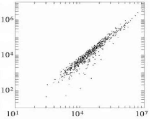
This constraining effect is clearly observable when plotting, on a logarithmic scale, the two components of a ratio. Figure 1 shows the constraint imposed by Total Assets on the spread of Net Worth.

Figure 1 Bivariate distribution of Total Assets (X-axis) and Net Worth (Y-scale).

Adequate transformations can take into account constraining mechanisms yielding unconstrained ratios. For example, any ratio where the numerator cannot be larger than the denominator, i.e., ratios of the form

∑

x x

can be transformed into the corresponding, unconstrained, ratio

i i i x x x −

∑

The unconstrained ratio corresponding to the ratio Fixed Assets to Total Assets (FA/TA) is the ratio FA/CA where CA=TA-FA. The information contained in both ratios is the same. The difference between them is just functional.

Table 1 summarises transformations able to bring ratios affected by several types of constraints into parametric behaviour. Ratios where there is no constraint are lognormal.

Table 1: Transformations adequate to be used in constrained ratios (from McLeay and Trigueiros, 2003).

Case No

Ratio Example Transformation to use

Boundaries of the ratio 1 R = Y/X Current Ratio Log R 0,∞ 2 R = (X-Y) / X Sales Margin Log (1-R) -∞,1 3 R = (Y-X) / X Change in Capital

Employed Log (1+R) -1,∞ 4 R = (Y+X) / X Interest Cover Log (R-1) 1,∞ 5 R = X / (Y+X) Liabilities Ratio Log (1 / R - 1) 0,1 6 R = X / (Y-X) Leverage Ratio Log (1 / R + 1) 0,∞

Awareness of the existence of constraining mechanisms and the way they affect ratios removes one major obstacle in understanding and using financial ratios. But not all is explained. A fact that remains unaccounted for is the existence of fat tails (leptokurtosis) in the logarithms of all types of ratios, that is, even after appropriate transformations are applied. Such leptokurtosis, though, is not severe and may, in most cases, be ignored.

Before moving on to the following section it is important to recall two facts about ratios. First, the use of ratios requires caution in order to avoid other, well-documented limitations. Ratios, for instance, produce ambiguous results when denominators, not only numerators, may take on negative values; ratios are sensitive to atypical magnitudes (numbers from the Profit and Loss account must be corrected for reported periods different from one year; accounts from the Balance Sheet may be distorted by seasonal effects). The second important fact is that, notwithstanding the above limitations, ratios do not deserve the negative image conveyed by scientific journals and books. In spite of their widespread use, ratios are regarded with scepticism by scholars and are described as some primitive tradition with no scientific support. One major cause of such scepticism is the mentioned diversity in statistical distributions. Another is the fact that some reported

numbers may take on negative values, which is difficult to reconcile with multiplicative behaviour.

The following section discusses the distribution of accounting flows or differences (such as Earnings) which may indeed take on negative values.

3. The Distribution of Earnings

The literature on the distribution of ratios seems to consider profits as additive, albeit not necessarily Normal (McLeay, 1986; Tippett, 1990; amongst others). Probably this is because authors focus on profitability ratios, not on profits.

Profitability ratios basically express percent changes in Net Worth. Authors believe that a ratio of the form dx/x should approach normality since lognormal x lead to Normal dx (where dx are small disturbances). However, in order to qualify as a small disturbance, dx must be really small when compared with x. Now, for most numbers taken from sets of accounts, this is simply not the case. Flows such as changes in Net Worth are not small enough to qualify as a disturbance, not least when compared with the respective stock. Annual Sales, in spite of being a flow, often is larger than stocks such as Fixed Assets, e.g., in high turnover industries. Actually, accounting flows are not that different from stocks, being large accumulations. Thus profitability and other ratios are indeed multiplicative.

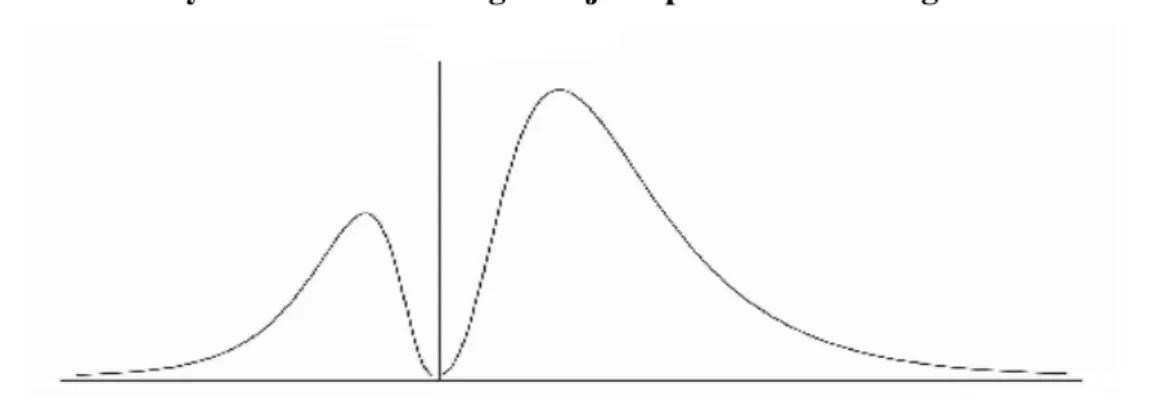
Numbers that may take on negative values are simply the result of subtracting positive-only accumulations. A magnitude reported as Earnings is obtained by subtracting the different types of costs and expenses from Revenues. The distribution of these variables should therefore stem from subtracting lognormal distributions. The task of analytically determining such distributions is not easy as it requires working out the logarithm of a subtraction. There is however a fact that simplifies analysis. Costs and Revenues are correlated because both are influenced by the same effect, size. When correlation is taken into account it becomes possible to approximate analytically the distribution of flows. It turns out that, for conditions typically found in industries, such distribution is not unique. Rather, it is a juxtaposition of two approximately lognormal density functions, one for positive and the other for negative values, the latter being a mirror-image of the lognormal as depicted in figure. Simulation confirms this result.

Figure 2: The density function of Earnings is a juxtaposition of two lognormal distributions.

Ratios formed with such distributions may be markedly two-tailed, giving the impression that they are near symmetry. Fat-tailed distributions such as Student's t or Cauchy's may indeed fit them closely (McLeay, 1986). It should be made clear, however, that the hypothesis of additive distributions leads to unreasonable conclusions. The reporting of immaterial values must be less likely than that of size-related values. The probability density of Earnings, for instance, must decrease when approaching zero and then increase again after passing through zero into negative values as predicted by Figure 2. This is because losses, as well as profits, must be proportionate to size. Additive distributions would imply that the reporting of immaterial profits or losses is more likely than that of material losses.

Ratios are multiplicative no matter their components' type, stocks or flows. When the ratio is constrained by some accounting identity, an appropriate transformation will bring it back to a standard behaviour. Specifically, profitability ratios will benefit from transformation 3 in Table 1. Indeed, most commonly found situations involving negative flows are solved simply by using this or other transformation. As for ratios where the denominator, not just the numerator, may take on negative values, it seems as though there is no other choice but to consider two populations, one for positive and the other for negative denominators. This, after all, is how practitioners deal with such ratios.

4. How to Account for Non-Proportionality in Ratios

Measurement using ratios requires proportionality between components. If the natural relationship between ratio components y and x is of the form y = a + bx (non-proportional) rather than y = bx (proportional), then the measurement will be misleading as y/x cannot have constant standards or norms (see, e.g., Lev and Sunder, 1979). The existence of non-proportional ratios is established by Sudarsanam and Taffler (1995) and by others.

How to overcome problems posed by non-proportionality? The Law of Proportionate Effect acknowledges that changes dx in (1) may be proportional, not to x itself, but to x - δ. In this case, the natural form governing the generation of reported magnitudes will be

dx

d dz

x−δ =µ τ + (2)

instead of (1). In turn, δ may be either constant or size-related. Constant δ stem, e.g., from the effect of fixed costs in a cost structure. Indeed, in a time series, the existence of fixed costs leads to a constant displacement in the distribution of Operating Costs. Size-related δ arise in similar cases in cross-section.

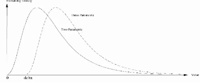
Where δ is constant, conditions leading to lognormal x in (1) generate, in (2), distributions known as three-parametric lognormal with threshold δ (Aitchison and Brown, 1957). Three-parametric lognormal density functions are simply the result of displacing lognormal distributions by δ (Figure 3).

Figure 3: The lognormal (solid line) and the three-parametric distributions (dashed line).

In order to cope with constant non-proportionality, one of the following ratios, δ − x y or x y δ− _,

should be used for, respectively, three-parametric lognormal numerators or denominators. Thresholds are δy or δx. Indeed, there exists a value of such δ for which the above,

non-proportional, ratios become proportional.

How damaging thresholds are for the ratio measurement? Due to the exponential character of (2), reported magnitudes may attain values many times larger than the threshold and, in such case, x - δx ≈ x. Non-proportionality is significant only where

magnitudes are not much larger than δ, for example, in the time-series context. Indeed, comparatively large size-independent thresholds are plausible only in such context.

periods. Values that are constant inside firms, such as fixed costs, may create comparatively large thresholds. In cross-section, as observations have their origin in different objects, size-independent thresholds would require the existence of industry-wide “fixed” costs. Since such costs should allow for the survival of small firms, they must be small. An industry-wide cost of £4m for food manufacturers in the UK would be only 0.2% of United Biscuits' revenues, but it would equal or exceed the turnover of the 5% smaller firms in the industry.

As mentioned, fixed costs are also likely to generate size-related thresholds, namely in cross section where large firms have large fixed costs and small firms have small fixed costs. In this case, the behaviour of δ is similar to that of any accounting variable where correlation with size is the rule. According to (2), x will be larger than expected for comparatively large δ, (e.g., the case of large firms) and x is not constant. As

a consequence, size-related thresholds do distort ratio measurement. Notice that the problem, in this case, is not any displacement in the distribution of ratio components. Since δ are small for small x and large for large x, distributions are not displaced. The problem is non-linearity in their relationship. Indeed, size-related thresholds require the use of ratios of the type

β

x y

.

For a specific value of β, the ratio will have a constant standard thus allowing measurement. On a logarithmic scale, the functional form of such measurement is

log y−βlogx=ρ+ z (3)

where ρ is the logarithm of the ratio standard and z is the observed deviation from that standard. (3) is similar to a regression. The slope β is approximate to the unit in the case of strict proportionality. Slopes smaller than 1 mean negative δ. In cross-section, they bias large firm's ratios downwards, mimicking scale effects.

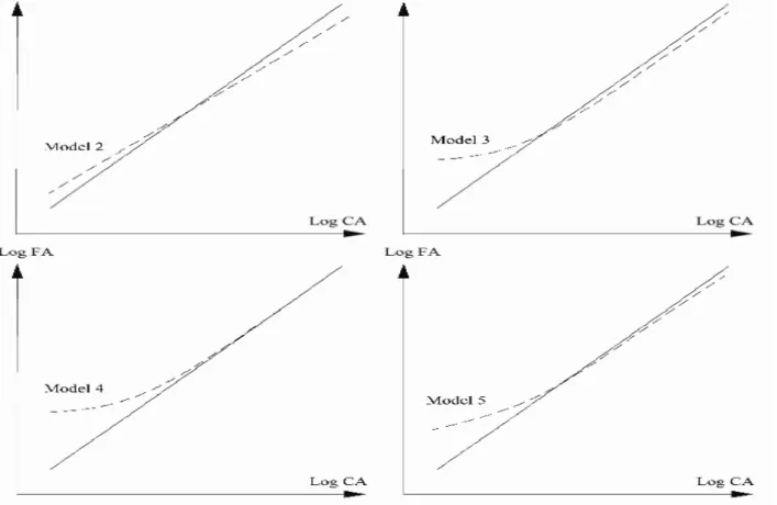
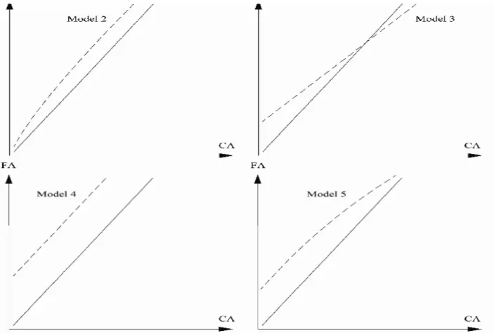
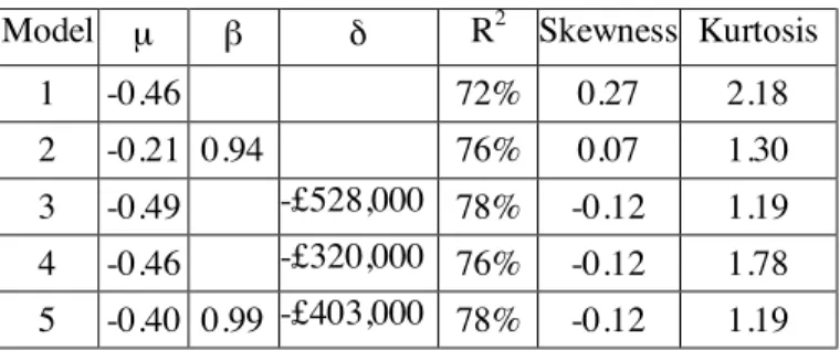
How should the two types of δ just outlined (constant and size-related) be estimated? The ratio Fixed Assets (FA) to Current Assets (CA) is now used in a cross-section example. Five models of ratio, as follows, are compared. Each model is presented together with its logarithmic counterpart as multiplicative formulations require logarithmic scaling prior to coefficient estimation. Figure 4 shows, on a logarithmic scale, how the usual ratio (solid line) compares with each model. Figure 5 reproduces figure 4 on the original scale (only the region near the origin is displayed).

Figure 4: The usual ratio (solid line) compared, on a logarithmic scale, with the slope ratio (Model 2), threshold ratios (Models 3 and 4), and the threshold plus slope ratio (Model 5).

Figure 5: The usual ratio (solid line) compared with the slope ratio (Model 2), threshold ratios (Models 3 and 4), and the threshold plus slope ratio (Model 5).

Model 1: the usual ratio, no correction introduced. This ratio requires the estimation of

one parameter, the standard. In cross-section, an appropriate standard is the median of the distribution of the ratio (on a logarithmic scale, µ). Therefore,

z w = + + =10 or logFA logCA CA FA µ µ

with z being a random disturbance and w = 10z When the distribution of CA and FA are nearly lognormal, the standard may be estimated by subtracting the averages of log FA and log CA. However, since a significant threshold in the distribution of CA is ignored, such standard will be misleading.

Model 2: ratio with size-related threshold in the denominator. This ratio may control

for the existence of economies of scale and other forms of non-linearity. It requires the estimation of two parameters, the standard (µ in logarithms) and the slope β. Regressions similar to (3) may be used to estimate both:

w z µ β β µ 10 CA FA ratio the to ing correspond CA log FA log = + + =

Graphically the ratio is a straight line on logarithmic scale and, as mentioned, it is non-linear on ordinary scale.

Model 3: ratio with constant threshold in the denominator (joint estimation). This

ratio corrects for a constant threshold but in such a way that the standard is corrected as well. It requires the estimation of two parameters: the standard (µ in logarithms) and δ, the constant threshold. Both are estimated using

. 10 CA FA ratio the to ing correspond ) CA log( FA log z µw δ δ µ = − + − + =

Graphically, the ratio is non-linear on logarithmic scale and a straight line on ordinary scale.

Model 4: ratio with constant threshold in the denominator (independent estimation).

In this case there is only one degree of freedom, µ, the logarithm of the ratio standard. The constant threshold of the distribution of CA, d, is estimated prior to that of the standard. µ is thus estimated using

. 10 CA FA ratio the to ing correspond ) CA log( FA log w d e d µ µ = − + − + =

Graphically, the ratio is non-linear and parallel with model 3 on logarithmic scale and straight on ordinary scale. This ratio probably is the most useful as non-proportionality is accounted for albeit converging with the usual ratio for medium-sized and large firms.

Model 5: ratio with both constant and size-independent thresholds. This ratio requires

the estimation of three parameters, µ, β and δ, using

. 10 ) CA ( FA to ing correspond ) CA log( FA log z µw β δ δ β µ = − + − + =

Graphically, the ratio is a mixture of models 2 and 3.

The independent estimation of a constant threshold (model 4) may be carried out using any of the procedures to detect three-parametric lognormality in distributions. In this example, δCA = -320,000 is estimated using the procedure suggested by Royston

Table 2 shows the variability explained (R2) by each of the five ratios. Skewness and kurtosis of residuals on a logarithmic scale (z) is also displayed. As can be seen, by allowing β into model 2, R2 approaches the variability explained by constant thresholds (models 3 and 4). Once δ is accounted for, β returns to an estimated value of nearly 1 (model 5).

Table 2: Parameters and statistics of the five models.

Model µ β δ R2 Skewness Kurtosis

1 -0.46 72% 0.27 2.18

2 -0.21 0.94 76% 0.07 1.30 3 -0.49 -£528,000 78% -0.12 1.19 4 -0.46 -£320,000 76% -0.12 1.78 5 -0.40 0.99 -£403,000 78% -0.12 1.19

Another example of the adequacy of threshold ratios may be taken from practice: time-series regressions where Operating Costs explains Sales are traditionally used to estimate Fixed Costs (the intercept term). Where the threshold ratio is used as an alternative to such regressions, the obtained estimates are clearly different in meaning. Where the correlation between Sales and Operating Costs is not very high, then the slope of the regression is clearly smaller than the ratio standard. In the limit, for a correlation approaching zero, such slope would also become zero and the intercept, which is supposed to estimate of Fixed Costs, would equal the expected value of Operating Costs. Regressions are thus inadequate for this task. They introduce in the estimation the spurious effect of correlation. By contrast, the threshold ratio correctly explains Fixed Costs as a displacement in the distribution of Operating Costs.

5. How to Model Firm Size

Firm size is often chosen as a substitute for numerous theoretical constructs, ranging from risk to liquidity or even political costs. Size is also an ingredient of its own in many theoretical models. In spite of this widespread use, size has remained a poorly defined concept. Where the use of size is required by theory, empirical studies typically revert to using proxies such as Total Assets, Market Capitalisation or Sales (see, e.g., Bujaki and Richardson, 1997).

The multiplicative character of magnitudes reported in accounts suggests, as stressed before, that the generation of their distribution is driven by size. It is indeed possible to deduce a simple and effective definition of firm size from the two following assumptions: first, reported magnitudes broadly obey the Gibrat's Law of Proportionate Effect; second, financial ratios do remove the effect of size.

In order for ratios to be effective, the likelihood of observed discrepancies in relation to the standard must be independent of size. For instance, the Return on Assets ratio is useless if an increase or decrease of 2% has different meanings for small and large firms. The probability distribution of ratios must therefore be homeoscedastic in terms of size. This implies, in the general case, that percent changes in both the numerator and denominator must be size-independent. As mentioned, variables where percent changes are size-independent are said to obey the Gibrat's Law of Proportionate Effect. Indeed, the widespread use of ratios agrees with the fact that reported numbers are multiplicative.

It was also mentioned that multiplicative mechanisms lead to broadly lognormal distributions. In fact, observed x generated as in (1) may be described functionally as

[1

]

x

X

=

+ x

As for the second assumption mentioned above, that of ratio y/x eliminating the effect of size, it leads to the requirement that the numerator y and denominator x should both be generated under the effect of equal rates of change (y = x). In fact, where y ≠ x the ratio standard would not be constant, showing a rate of change of y/x with τ. This requirement importantly suggests that, not just y and x but the other numbers found in a specific annual report, are generated under the effect of the same rate of change. Indeed, the validity of the ratio method rests on the validity of several, widely used ratios (not just on one or two cases), where numbers used to form one of such ratios are also used to form other ratios. Therefore, if ratios are to be of any use, there must exist a common source of variability underlying numbers reported in the accounts of a firm in a given year. Where numbers x1, x2,..., xk,... all belong to a specific annual report, this assumption leads to x1 =

x2 = …= xN. It is possible to show that such unique source of variability possesses the

attributes of size.6

How can size be estimated from this rate of change? A specific annual report, say, report j, is characterised by what value τ assumes xk, the magnitude reported by item k, is

explained as

exp [

]

K K j

where xjτ is the effect of size (the same for all items reported in j). In an additive form,

log xK=µK +σj+z (5)

where µ k = log Xk and σj =xjτ. Formulation (5) is basically an Analysis of Variance, i.e.,

a type of linear model aimed at explaining variability in terms of membership of discrete classes. Specifically, in (5) log xk is explained by its membership of two classes, the item

class, µ k, and the annual report class, σj. The item class is a fixed (deterministic) effect,

as it denotes the fact that k is a specific item amongst those in the sets of accounts reported by firms. These accounts are indeed fixed in number and in type. By contrast, the annual report's class is a random effect: it denotes the fact that j is one of the (randomly selected) annual reports in the sample. Each of these two classes possesses levels, namely, there can be as many levels of k as items in the sets of accounts; there can be as many levels of j as different reports in the sample.

In cross section, µk is the expected value of logarithmic magnitudes reported in

item k, estimated as the mean of k calculated using all the annual reports in the sample. Thus, in this case, Xk in (5) is the median of magnitudes reported in k. The size effect, σj,

is the expected log xk - µk for numbers in j and its estimation is straightforward: given N

numbers, all of them reported in j, (5) is first applied to each of these numbers. The N formulations obtained are then added. Since σj is the same in all of these formulations, it

is possible to write σj = 1 (log ) 1 k N k k x N

∑

_∑

Any source of variability common to all log xk in j is, by construction, accounted

for by σj. Therefore, even where correlation amongst some z may exist, the term

∑

should tend to zero with an increasing N, leading to: Estimate of σj = 1 (log ) 1 k N k k x N

∑

An estimated size may thus be obtained simply by averaging the logarithms of appropriately adjusted magnitudes drawn from the firm's actual report. Exact confidence intervals for σj can also be obtained, the corresponding standard errors being t-distributed

with N-1 degrees of freedom.

The estimation of σj faces two obvious difficulties. First, xk cannot be drawn from

all possible accounts because items such as Earnings, being a subtraction, may take on negative values and cannot be transformed into logarithms. This pre-selection of items introduces a bias in the estimation of size. Second, inside each annual report, some z are correlated. This increases the standard error. In practice, however, size can be estimated with accuracy by averaging the logarithms of positive-only magnitudes such as Cash and

Short Term Investments, Receivables, Total Inventories, Property, Plant and Equipment (net), Common Equity, Number of Employees, Net Sales, Cost of Goods Sold (excluding Depreciation), Depreciation of the year, Interest Expense and others.

6. Concluding Remarks

Accounting data obeys a set of simple rules. The first rule states that, since reported numbers and ratios are multiplicative, logarithmic transformations should be used to bring data to additive behaviour. The second rule explains that accounting identities often distort otherwise multiplicative distributions of ratios into unexpected shapes. Such identities should be accounted for prior to logarithmic transformation. The third rule explains the different ways to account for non-proportionality in ratios. The fourth rule states that numbers in a specific report are generated under the influence of size, being possible to obtain a size estimate just by averaging several of these numbers, conveniently adjusted. The distribution of Earnings and the development of two-dimensional tools for analysis were also discussed.

It may be asked why so many contributions to the literature have led to a pessimistic view of ratios and accounting data in general. Reasons seem to relate to an apparent lack of theoretical drive, probably fed by an a priori conviction that accounting data should be complex and full of exceptions, just as the production of such data is indeed complex and full of exceptions. It is expected that, by using suggestions from this note, researchers and practitioners may find that such a priori conviction is, after all, a tradition with no scientific support.

References

Aitchison, J. and Brown, J.(1957), The Lognormal Distribution, (Cambridge University Press). Eisenbeis, R. (1977), `Pitfalls in the Application of Discriminant Analysis in Business, Finance

and Economics', The Journal of Finance, Vol.32, No.3, pp.875-899.

Lev, B. and Sunder, S. (1979), `Methodological Issues in the Use of Financial Ratios', Journal of Accounting and Economics, December, pp.187-210.

McLeay, S. (1986), `The Ratio of Means, the Mean of Ratios and Other Benchmarks', Finance, Journal of the French Finance Society, Vol.7, No.1, pp.75-93.

McLeay, S. and Trigueiros, D. (2002), `Proportionate Growth and the Theoretical Foundations of Financial Ratios', Abacus, Vol.XXXVIII, No.3, pp.297--316.

Royston, J. (1982), `An Extension of the Shapiro and Wilk's Test for Normality to Large Samples', Applied Statistics, Vol.31, No.2, pp.115--124.

So, J. (1987), `Some Empirical Evidence on Outliers and the Non-Normal Distribution of Financial Ratios', Journal of Business Finance and Accounting, Vol.14, No.4, pp.483--495.

Sudarsanam, P. and Taffler, R. (1995), `Financial Ratio Proportionality and Inter-Temporal Stability: An Empirical Analysis'. Journal of Banking and Finance, Vol.XIX, pp.45--60. Tippett, M. (1990), `An Induced Theory of Financial Ratios', Accounting and Business

Research, Vol.21, No.81, pp.77-85.

Trigueiros, D. (1995), `Accounting Identities and the Distribution of Ratios', British Accounting Review, Vol.27, No.2, pp.109-126.

Notes

1. Natural forms describe mechanisms rather than observations. They are often expressed as differential or as difference equations.

2. Eisenbeis (1977) mistakenly stated that `log-transformed variables give less weight to equal percentage changes in a variable where the values are large than when they are smaller. The implication would be that one does not believe that there is as much difference between a $1 billion and a $2 billion size firms as there is between a $1 million and a $2 million size firms. The percentage difference in the log will be greater in the latter than in the former case' (p. 877). Eisenbeis' pitfall is that the calculation of proportions of the log-transformed measurement is equivalent to calculating proportions twice. This inappropriate warning against logarithmic transformations gave support at the time to the use of ad hoc techniques such as those proposed by Frecka and Hopwood (1983).

3. The coefficient of variation is the standard deviation expressed as a fraction of expected value.

4. Royston uses trial and error to find out which δ maximises the parameter W of the Shapiro and Wilk's test of normality.

5. (1) may not necessarily lead to (4). Indeed, the simplest formulation generated by (1) is xk = Xk exp [(xj – σ2/2)τ + z]

rather than (4). Since the compounding effect is now influenced by the standard deviation of z, not just by size, this variable is non-proportional and cannot be used to form ratios. In case, however, of continuously compounding rates of change, then a proportional mechanism is obtained