ISSN 1546-9239
© 2012 Science Publications
Corresponding Author: Muhammad Hisyam Lee,Department of Mathematics, Faculty of Science, Universiti Technology Malaysia, 81310, Skudai, Johor, Malaysia
570
Seasonal ARIMA for Forecasting Air Pollution Index: A Case Study
1
Muhammad Hisyam Lee,
1Nur Haizum Abd. Rahman,
2Suhartono,
3Mohd Talib Latif,
1Maria Elena Nor and
1Nur Arina Bazilah Kamisan
1Department of Mathematics, Faculty of Science,
Universiti Technology Malaysia, 81310, Skudai, Johor, Malaysia
2Department of Statistics, Faculty of Mathematics and Natural Sciences,
Institute Technology Sepuluh Nopember, Surabaya 60111, Indonesia
3
School of Environmental and Natural Resource Sciences,
Faculty of Science and Technology, University Kebangsaan Malaysia,
43600 Bangi, Selangor Malaysia
Abstract: Problem statement: Both developed and developing countries are the major reason that affects the world environment quality. In that case, without limit or warning, this pollution may affect human health, agricultural, forest species and ecosystems. Therefore, the aim of this study was to determine the monthly and seasonal variations of Air Pollution Index (API) at all monitoring stations in Johor. Approach: In this study, time series models will be discussed to analyze future air quality and used in modeling and forecasting monthly future air quality in Malaysia. A Box-Jenkins ARIMA approach was applied in order to analyze the API values in Johor. Results: In all this three stations, high values recorded at sekolah menengah pasir gudang dua (CA0001). This situation indicates that the most polluted area in Johor located in Pasir Gudang. This condition appears to be the reason that Pasir Gudang is the most developed area especially in industrial activities. Conclusion: Time series model used in forecasting is an important tool in monitoring and controlling the air quality condition. It is useful to take quick action before the situations worsen in the long run. In that case, better model performance is crucial to achieve good air quality forecasting. Moreover, the pollutants must in consideration in analysis air pollution data.
Key words: Air Pollution Index (API), time series modeling, ARIMA time series, air quality forecasting, pollution data
INTRODUCTION
Both developed and developing countries especially in Europe, America and Asia contribute more in world environmental air quality status (Karatzas et al., 2008). This air pollution can be found both either indoors, occur when the pollutants trapped in the buildings that could last for a long time or outdoors which the pollution located in the atmosphere. For this reason, the pollutants can transport pollution travel far from the origin to other places easily. Therefore, air pollution is one of the major issues in the world and become the fundamental pollution problem in many parts of the world (Kurt and Oktay, 2010).
This air pollutant usually caused by two main factors, human-based factor such as open burning, industrial processes, fuel burning vehicle and may also
by natural disaster like volcanoes Department of Environment 2004 (Kalantari et al., 2007; Pires et al., 2008). Series of air pollution recorded all over the world create the principal cause of dangerous effect on human health for short term consequences. Meanwhile, air pollution tends to increase earth risk on global warming and greenhouse in long term consequences (Kurt and Oktay, 2010).
As for Malaysia, Department of Environment (DOE), Malaysia is responsible in monitoring and managing Malaysia’s ambient air quality through a network of 51 stations. Meanwhile, Alam Sekitar Malaysia Sdn. Bhd. (ASMA) is an important organization that responsible in collecting the air pollution data for DOE. For this study, monthly data of API in Johor from 2000-2009 are analyzed. These 10 years monthly mean API data covers three stations located at Sekolah Menengah Pasir Gudang Dua (CA0001), Sekolah Menengah Vokasional Perdagangan Johor Bahru (CA0019) and Sekolah Kebangsaan Ismail Dua, Muar (CA0044).
Given that all of the data are generated accordingly in the form of a time series. For that reason, in order to analyse the air quality, time series modelling and forecasting is chosen in this study. This approach is selected to be used in air quality management to help making future planning and helps to shape the better air quality since time series analysis is the major task for researchers used in development (Cryer and Chan, 2008). As for Malaysia, the research and development of time series modelling and forecasting for monitoring air pollution are still limited.
MATERIALS AND METHODS
By using time series, this study aims to analyse the API performance. The time series approach used in this study is based on Box-Jenkins model. Box-Jenkins is referred as Autoregressive Integrated Moving Average (ARIMA) method. Until nowadays, a lot of researchers still use this model in many area of research because the result effectiveness in forecasting field (Wang and Lu, 2006; Ibrahim et al., 2009; Kumar and Jain, 2010). Sampling sites: The Southern Region of Peninsular Malaysia, Johor has been chosen as the study site ASMA, 2006. There are four air quality monitoring stations located in Johor. However only three monitoring stations, namely as Sekolah Menengah Pasir Gudang Dua (CA0001), Sekolah Menengah Vokasional Perdagangan Johor Bahru (CA0019) and Sekolah Kebangsaan Ismail Dua, Muar (CA0044) has been chosen in this study. This is because the data obtain from monitoring station in Sekolah Menengah Kebangssan Perling, Tampoi (CA0051) has been eliminated since the monitoring station change from Tampoi to Kota Tinggi in 2008. This make the data not valid to be included in this study within the time range stated. Between these three stations, station located at Pasir Gudang is an industrial town make the human-based factors increase. As the result, Pasir Gudang recorded as the highest polluted area in Johor.
Air pollution index: The Air Pollution Index (API) is a simple generalized way in describing the air quality status. It was calculated based on five main sets of air pollutants concentration namely Particulate Matters (PM10), Sulphur Dioxide (SO2), Nitrogen Dioxide (NO2), Carbon Monoxide (CO) and Ozone (O3). Then the daily API value recorded will be based the highest index value. The air pollutant index scale and terms used in describing the air quality levels are shown in Table 1.
Box-Jenkins modeling: The Box-Jenkins is taken in honour of its discoverers, Box and Jenkins (1976). This method is classified as linear models that capable in presenting both stationary and non-stationary time series. Most of researchers use this model to forecast univariate time series data. Box-Jenkins methods is a practical importance in forecasting which inclusive Autoregressive (AR) models, the Integrated (I) models and the Moving Average (MA) models (Cryer and Chan, 2008).
To obtain the model by the Box-Jenkins methodology, there are four steps that must be considered which are tentative identification, parameter estimation, diagnostic checking and finally model is used in prediction purposes. This step is the important procedure in order to determine the best ARIMA model for time series data (Hanke and Wichern, 2008).
Autoregressive (AR), Moving Average (MA) and Autoregressive Integrated Moving Average (ARIMA) Models: Autoregressive (AR) model is suitable for stationary time series data patterns. A pth-order of autoregressive or AR (p) model can be written in the form Eq. 1:
t 0 1 t 1 2 t 2 p t p t
Y = φ + φY− + φY− +…+ φY− +ε (1)
The current value of the series yt is a linear combination of the p most recent values of itself. The coefficient φ0 is related to the constant level of series.
For AR models, forecast depend on observed values in previous time periods. Meanwhile, the dependent variable yt of Moving Average (MA) depends on previous values of the errors rather than on the variable itself. MA models provide forecasts of yt based on linear combination of a finite number of past errors. The errors involved in this linear combination move forward as well.A moving average with qth-order or MA (q) model takes the form Eq. 2:
t t 1 t 1 2 t 2 q t q
572 Table 1: Air Pollution Index (API)
API scale Air quality
0-50 Good
51-100 Moderate
101-200 Unhealthy
201-300 Very unhealthy
301 and above Hazardous
A mixed between autoregressive and moving average terms develop Autoregressive moving Average Model (ARMA). The notation is ARMA (p, q) where, p is the order of the autoregressive part and q is the order of the moving average part which represent this models. The ARMA (p,q)) is in the form below Eq. 3:
t 0 1 t 1 2 t 2 p t p
t 1 t 1 2 t 2 q t q
Y Y Y Y
ε θ ε θ ε θ ε
− − −
− − −
= φ + φ + φ +…+ φ
+ − − −…− (3)
A wide variety of behaviors for stationary time series can be described by ARMA models. Since ARMA is a mixture of AR and MA, the forecasting is depend on both current and past values of response Y as well as current and past values of the residuals.
Set of data could be a non-stationary time series data patterns since the data did not fluctuate around a constant level or mean. One way to make the data stationary is by taking the difference. Therefore, the series of data generally donated as yt after difference is said to follow an integrated autoregressive moving average model, ARIMA (p, d, q). Normally for practical purpose, the difference would be one or at most two (d≤2).
By considering d = 1, we can obtain ARIMA (p,1,q) process with dyt=Wt or may written as Wt=yt− yt−1. Then, (3) becomes Eq. 4:
t 1 t 1 2 t 2 p t p t 1 t 1 2 t 2 q t q
W W W W
ε θ ε θ ε θ ε
− − −
− − −
= φ + φ + …+ φ +
− − −…− (4)
Rewrite (3) as Eq. 5:
(
)
(
)
(
)
t 1 t 1 2 1 t 2 3 2 t 3
p p 1 t p p t p 1 t 1 t 1 2 t 2 q t q
Y 1 Y Y Y
( )Y Y ε
θ ε θ ε θ ε
− − −
− − − −
− − −
= + φ + φ − φ + φ − φ +…
+ φ − φ − φ + −
− −…−
(5)
Seasonal ARIMA model (SARIMA): The Box-Jenkins approach for modeling and forecasting has the advantage in analyze the seasonal time series data. In this case where the seasonal components are included, the model is called as seasonal ARIMA model or SARIMA model.
The model can be abbreviated as SARIMA (p, d, q) (P, D, Q)S where the lowercase for non-seasonal part meanwhile the uppercase for seasonal part. The generalized form of SARIMA model can be written as Eq. 6:
( )
( )
s d S D( )
Sp B ΦP B (1 B) (1 B ) Yt θq B ΘQ(B) εt
φ − − = (6)
Where:
( )
( )
( )
( )
2 pp 1 2 p
S 2S PS
P 1 2 P
2 q
q 1 2 q
S 2S QS
Q 1 2 Q
B 1 B B B
Φ B 1 ΦB ΦB Φ B
θ B 1 θB θB θ B
Θ B 1 ΘB ΘB Θ B
φ = − φ − φ −…− φ
= − − −…−
= − − −…−
= − − −…−
Measure of accuracy: For identification of the models performance, the criteria chosen are the Mean Absolute Error (MAE), the Mean Absolute Percentage Error (MAPE), the Mean Square Error (MSE) and the Root Mean Square Error (RMSE). Given as:
n t t t 1Y Y MAE n = − =
∑
ɵ t t n t 1 t Y Y YM APE 10
n = − = ×
∑
ɵ n 2 1 t t Yt YM SE n = − =
∑
ɵ 2 n t t i 1 Y Y RM SE n = − =∑
ɵ Where:yt = The actual value at time t t
y
⌢ = The fitted value at time t
n = The number of observations
The smallest values of MAE, MAPE, MSE and RMSE are chosen as the best model to be used in forecasting.
RESULTS
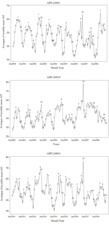
574 API raw data plots: The data used in this study obtained from Johor continuous air quality monitoring located at Sekolah Menengah Pasir Gudang 2 (CA0001), Sekolah Menengah Vokasional Perdagangan (CA0019) and Sekolah Kebangsaan Ismail Dua, Muar (CA0044) from January 2000-December 2009.
The data divided into two samples data set, in sample and out sample. The in sample data set contains 108 data (January 2000 until December 2008) meanwhile the last 12 data (January until December 2009) as out sample used to test the model performance. The time series plots of these three stations are shown in Fig. 1 with the air quality recorded for this station within good and moderate health condition.
The time series plot illustrate that the data have seasonal pattern which indicates that the data non-stationary (Hanke and Wichern, 2008). In that case, the differencing process is necessary to obtain the stationary data set before model development can be made. By taking difference d = 1 for non-seasonal and D = 1 with S = 12 for seasonal then the data become stationary series. As stated before, there are three main stages in building ARIMA model before used in forecasting, tentative identification, parameter estimation and diagnostic checking.
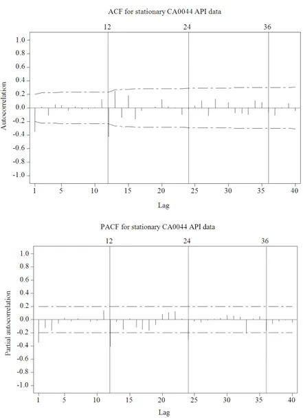
Model identification: Based on stationary series, the Autocorrelation (ACF) and Partial Autocorrelation (PACF) were examined to determine the best combination order of ARIMA model for each data set. The ACF and PACF of each data set shows in Fig. 2. The possible models are:
Sekolah Menengah Kebangsaan Pasir Gudang Dua, (CA0001):
SARIMA (0, 1, 1) (1, 1, 0)12 SARIMA (0, 1, 1) (0, 1, 1)12
Sekolah Menengah Vokasional Perdagangan Johor Bahru (CA0019):
SARIMA (1, 1, 0) (1, 1, 0)12 SARIMA (1, 1, 0) (0, 1, 1)12 SARIMA (0, 1, 1) (1, 1, 0)12 SARIMA (0, 1, 1) (0, 1, 1)12
Sekolah Kebangsaan Ismail Dua, Muar (CA0044): SARIMA (1, 1, 0) (1, 1, 0)12
SARIMA (1, 1, 0) (0, 1, 1)12 SARIMA (0, 1, 1) (1, 1, 0)12 SARIMA (0, 1, 1) (0, 1, 1)12
When the tentative model is identified, the next step is to achieve the most efficient estimates of the parameters. Model estimation: Then, based on ARIMA model, the arameter of each coefficient in AR and MA for both
seasonal and non-seasonal can be identified. However, before choosing the coefficient values, the estimation output must satisfy the significant criteria in the next step, model checking.
Model checking and forecasting: By using Ljung-Box test and checking the p-value of the coefficient, then the significant model can be determined. Without taking the constant value into the model, the possible model stated for each station satisfied both of these tests.
Then, the process continues to calculate the forecasting values based on satisfied model. The result shows in Table 2-4.
Forecasting ARIMA model: The best model is chosen based on the smallest values of accuracy measurement. As for station CA0001 and CA0044, the best model to describe the API trend is the same, i.e., SARIMA (0, 1, 1) (0, 1, 1)12. The model can be written as:
t t 1 t 12 t 13 t t 1 t 12 t 13
Y =Y− +Y− −Y− + −ε θε− −Θε− +Θθε−
Meanwhile, the API model for station CA0019 is SARIMA (1, 1, 0) (0, 1, 1)12. Thus, the model equation is:
t t 1 t 12 t 12 t 13 t 13 t 14 t t 12
Y =Y− +Y− + φY− −Y− − φY− − φY− + −ε Θθε−
Based on this final model for each station, it will be used in forecasting API values within in-sample and out-sample data set.
DISCUSSION
Based on the result shows in Table 2-4, it shows the performance by using ARIMA model in forecasting out-sample data set. In general, this ARIMA method is capable in monitoring the air pollution situation.
Table 2: Out-Sample forecasting performance in station CA0001 Model MAPE MAE MSE RMSE SARIMA (0, 1, 1) (0, 1, 1)12 11.0793 5.3910 37.7595 6.1449
SARIMA (0, 1, 1) (1, 1, 0)12 11.8042 5.7694 44.4996 6.6708
Table 3: Out-Sample forecasting performance in station CA0019
Model MAPE MAE MSE RMSE
SARIMA (1, 1, 0) (1, 1, 0)1215.2816 7.0643 76.0499 8.7207 SARIMA (1, 1, 0) (0, 1, 1)12 9.9936 4.1238 21.8991 4.6796 SARIMA (0, 1, 1) (1, 1, 0)1219.1304 8.8687 120.6870 10.9858 SARIMA (0, 1, 1) (0, 1, 1)12 9.7684 4.2197 23.8244 4.8810
Table 4: Out-Sample forecasting performance in station CA0044
Model MAPE MAE MSE RMSE
576
Fig. 3: Averages of monthly mean API in stations CA0001, CA0019 and CA0044 The actual values and predicted values time
series plot for stations CA0001, CA0019 and CA0044 shown in Fig. 3.Moreover, based on time series plot in Fig. 3, it also demonstrate the capability of ARIMA model in analysis the seasonal data pattern occurred in air quality which is the comparison between actual and predicted values.
Additionally, based on the time series plot for these three stations in Fig. 2, it generally show that the API values within the consideration values, good and moderate between 30-80. The time series plot for API forecasting model in Sekolah Menengah Pasir Gudang Dua (CA0001), the seasonality data recorded is more stable without any extreme value compared to the other stations.
As demonstrate in Fig. 2, in October 2006, there are extreme values clearly shown in station CA0019 and CA0044. According to annually DOE report, Malaysia experienced short periods of slight to moderate haze from July until October mainly due to trans boundary pollution Department of Environment, 2006.
CONCLUSION
578 By looking at the accuracy measurement in final model chosen, high values recorded at Sekolah Menengah Pasir Gudang Dua (CA0001). This situation indicates that the most polluted area in Johor located in Pasir Gudang. This condition appears to be the reason that Pasir Gudang is the most developed area especially in industrial activities.
In summary, the time series model used in forecasting is an important tool in monitoring and controlling the air quality condition. It is useful to take quick action before the situations worsen in the long run. In that case, better model performance is crucial to achieve good air quality forecasting. Moreover, the pollutants must in consideration in analysis air pollution data.
ACKNOWLEDGMENT
This study was supported by the Universiti Technology Malaysia, Malaysia, under Grant Q.J13000.7113.01H11. We like to thanks the Department of Environment (DOE), Malaysia for providing pollutants data.
REFERENCE
Afroz, R., M.N. Hassan and N.A. Ibrahim, 2003. Review of air pollution and health impacts in Malaysia. Environ. Res., 92: 71-77. DOI: 10.1016/S0013-9351(02)00059-2
Box, G.E.P and G.M. Jenkins, 1976. Time Series Analysis: Forecasting and Control. 1st Edn., Holden-Day, San Fransisco, ISBN:10: 0816211043, 575.
Cryer, J.D. and K.S. Chan, 2008. Time Series Analysis with Applications in R. 2nd Edn., Springer, New York, ISBN: 10: 0387759581, 491.
Hanke, J.E. and D.W. Wichern, 2008. Business Forecasting. 9th Edn., Pearson/Prentice Hall, Upper Saddle River, N.J., ISBN-10: 0132301202, pp: 551.
Ibrahim, M.Z., R. Zailan, M. Ismail and M.S. Lola, 2009. Forecasting and time series analysis of air pollutants in several area of Malaysia. Am. J.
Environ. Sci., 5: 625-632.
DOI:10.3844/ajessp.2009.625.632
Kalantari, K., H.S. Fami, A. Asadi and H.M. Mohammadi, 2007. Investigating factors affecting environmental behaviour of urban residents: A case study in Tehran city-Iran. Sci. Technol. Sustainab. Middle East North Africa, 6: 355-368.
Karatzas, K.D., G. Papadourakis and I. Kyriakidis, 2008. Understanding and forecasting atmospheric quality parameters with the aid of ANNs. Proceedings of the IEEE International Joint Conference on Neural Networks, Jun. 1-8, IEEE Xplore Press, Hong Kong, pp: 2580-2587 DOI: 10.1109/IJCNN.2008.4634159
Kumar, U. and V.K. Jain, 2010. ARIMA forecasting of ambient air pollutants (O3, NO, NO2 and CO). Stochastic Environ. Res. Risk Assessment, 24: 751-760. DOI: 10.1007/s00477-009-0361-8 Kurt, A. and A.B. Oktay, 2010. Forecasting air
pollutant indicator levels with geographic models 3 days in advance using neural networks. Expert Syst. Appli., 37: 7986-7992. DOI: 10.1016/j.eswa.2010.05.093
Pires, J.C.M., F.G. Martins, S.I.V. Sousa, M.C.M. Alvim-Ferraz and M.C. Pereira, 2008. Prediction of the daily mean pm10 concentrations using linear models. Am. J. Environ. Sci., 4: 445-453. DOI:10.3844/ajessp.2008.445.453
Siew, L.Y., L.Y. Chin and P.M.J. Wee, 2008. ARIMA and Integrated ARFIMA models for forecasting air pollution index in shah alam, selangor. Malaysian. J. Analytical Sci. 12: 257-263.