On Supervised multilinear filtering: applications to system and antenna beamforming

(1)

Federal University of Ceará

Department of Teleinformatics Engineering

Postgraduate Program in Teleinformatics Engineering

On Supervised Multilinear Filtering:

Applications to System Identification and

Antenna Beamforming

Master of Science Thesis

Author

Lucas Nogueira Ribeiro

Advisor

Prof. Dr. João César Moura Mota

Co-Advisor

Prof. Dr. André Lima Férrer de Almeida

(2)

Universidade Federal do Ceará

Departamento de Engenharia de Teleinformática

Programa de Pós-graduação em Engenharia de Teleinformática

Sobre a Filtragem Multilinear Supervisionada:

Aplicações em Identificação de Sistemas e

Formatação de Feixes de Antenas

Autor

Lucas Nogueira Ribeiro

Orientador

Prof. Dr. João César Moura Mota

Co-Orientador

Prof. Dr. André Lima Férrer de Almeida

Dissertação apresentada à Coorde-nação do Programa de Pós-graduação em Engenharia de Teleinformática da Universidade Federal do Ceará como parte dos requisitos para obtenção do grau de Mestre em Engenharia de Teleinformática. Área de

concen-tração: Sinais e sistemas.

(3)

Dados Internacionais de Catalogação na Publicação Universidade Federal do Ceará

Biblioteca de Pós-Graduação em Engenharia - BPGE

R369o Ribeiro, Lucas Nogueira.

On supervised multilinear filtering: applications to system identification and antenna beamforming / Lucas Nogueira Ribeiro. – 2016.

85 f. : il. color. , enc. ; 30 cm.

Dissertação (mestrado) – Universidade Federal do Ceará, Centro de Tecnologia, Departamento de Engenharia de Teleinformática, Programa de Pós-Graduação em Engenharia de Teleinformática, Fortaleza, 2016.

Área de concentração: Sinais e Sistemas. Orientação: Prof. Dr. João César Moura Mota.

Coorientação: Prof. Dr. André Lima Férrer de Almeida.

1. Teleinformática. 2. Tensores. 3. Identificação de sistemas. 4. Antenas. I. Título.

(4)

(5)

Abstract

Linear filtering methods are well known and have been successfully applied to many engineering problems. However, they become unpractical when the param-eter space is very large. The recently proposed assumption of system separability allows the development of computationally efficient alternatives to classical fil-tering methods in this scenario. In this work, we show that system separability calls for multilinear system representation and filtering. Based on this parallel, the proposed filtering framework consists of a multilinear extension of the clas-sical Wiener-Hopf (WH) filter that exploits the separability property to solve the supervised multilinear filtering problem. System identification and antenna beamforming computer simulations were conducted to assess the performance of the proposed method. Our numerical results show our approach has smaller computational complexity and that it provides better estimation accuracy than the classical WH filter, which ignores the multilinear system structure.

(6)

Resumo

Métodos de filtragem linear estão bem estabelecidos e têm sido aplicados em diversos problemas de engenharia. Entretanto, eles tornam-se impraticáveis quando o espaço de parâmetros é grande. A recente hipótese de separabilidade de sistema permite o desenvolvimento de métodos computacionalmente eficientes neste cenário. Neste trabalho, nós mostramos que a separabilidade de um sis-tema leva à sua representação multilinear. Em vista disso, o método de filtragem proposto consiste em uma extensão multilinear do filtro de Wiener-Hopf (WH) clássico, que explora a separabilidade para resolver o problema de filtragem mul-tilinear supervisionada. Simulações computacionais de identificação de sistemas e formatação de feixes de antenas foram realizadas para a avaliação do desempenho do método proposto. Nosso resultados numéricos mostram que nossa abordagem possui menor complexidade computacional e que ela fornece melhor acurácia de estimação que o filtro de WH clássico, que ignora a estrutura multilinear do sis-tema.

(7)

Acknowledgments

I would like to express my deepest gratitude towards: – God, for taking care of me;

– My family, for always supporting me; – Priscilla, for the love;

– CAPES, for the financial support;

(8)

List of Acronyms

ALS Alternating Least Squares CDMA Code Division Multiple Access FIR Finite Impulse Response

FLOPS Floating-point Operations Per Second

LMS Least Mean Square

MMSE Minimum Mean Square Error

MSE Mean Square Error

NLMS Normalized Least Mean Square PARAFAC Parallel Factors

PNLMS Proportionate Normalized Least Mean Square QPSK Quadrature Phase-Shift Keying

SepWH Separable Wiener-Hopf SNR Signal-to-Noise Ratio SOI Signal of Interest

STAP Space-Time Adaptive Processing TLMS Tensor Least Mean Square

TWH Tensor Wiener-Hopf

WH Wiener-Hopf

(9)

List of Symbols

 Square root of−1 Z _{Field of integer numbers} R _{Field of real numbers} C _{Field of complex numbers} E_[_·_] _{Statistical expectation} (·)H _{Hermitian operator}

(·)T _{Transpose operator}

·:=· Definition

Θ(·) Tensorization operator vec(·) Vectorization operator

· ◦ · Outer product

· ⊗ · Kronecker product

· ×n· n-mode product

h·,·i Inner product

k·k_F Frobenius norm

k · k2 Euclidean norm

· ⊔N · Tensor concatenation along the Nth dimension

· ∗ · Discrete-time convolution

(10)

List of Figures

2.1 Supervised linear filtering model. . . 7

2.2 Supervised multilinear system identification model. . . 16

2.3 Extended subsystem factorization example. . . 18

2.4 Separable Wiener-Hopf algorithm structure. . . 19

2.5 Identification of each extended subsystem of h using the SepWH algorithm. . . 20

3.1 Supervised system identification model. . . 25

3.2 Filtering methods performance as a function of the sample size for N = 1000 and SNR = 10dB. The step size of the adaptive filtering methods was set to µ= 10−2_{. . . 29}

3.3 Filtering methods performance as a function of the filter length for K = 35.000 samples and SNR = 10dB. The step size of the adaptive filtering methods was set to µ= 10−2_{. . . 30}

3.4 Filtering methods performance as a function of the SNR for K = 35.000 samples and N = 1000. The step size of the adaptive fil-tering methods was set to µ= 10−2_. _{. . . 31}

3.5 MSE performance for µ= 10−2_, _K _{= 35}_.₀₀₀ _samples, _N _{= 1000}_, and SNR = 30dB. . . 32

3.6 TLMS learning curves compared to the performance of the WH fil-ter and TWH algorithm forK = 3×105_,_N _{= 1000}_{, and SNR=}₁₀_{dB. 32} 3.7 TWH performance for varying separability orders and sample size, N = 1024 and SNR = 10dB. . . 33

(11)

3.9 TWH performance for varying separability orders and filter lengths according to the dimensions at Table 3.2,K = 35.000samples and SNR = 10dB. . . 35 3.10 TWH performance for varying separability orders and SNR,K =

35.000 samples andN = 1024. . . 36 4.1 A 4×2×2 volumetric array decomposed into three equivalent

forms. Reference subarrays are indexed by m= 1, whereasm >1

refers to translation. . . 41 4.2 Illustration of the antenna array factorization considered in the

computational simulations for N = 256 sensors. . . 43 4.3 Performance for a varying number of samples, N = 128 sensors

and SNR = 15dB. . . 45 4.4 Performance for a varying number of sensors, K = 5000 samples

(12)

Chapter 1 Introduction

The filtering problem consists of designing a set of parameters which extract information from a set of noisy data [1]. A filter can be mathematically repre-sented by a function that transforms an input signal into an output signal. A filter is classified with respect to the mathematical properties of its model: lin-ear or non-linlin-ear, instantaneous (memoryless) or dynamic (with memory), time variant or invariant, among others [2]. The statistical approach to the filtering problem consists of designing a filter that minimizes the error between its output signal and a given desired signal. In system identification problems, for instance, a filter is employed to model an unknown system. In this context, both devices are fed by the same input signal, and the output signal produced by the unknown system is regarded as the desired signal. The unknown system model parame-ters can be identified by minimizing the mean square error between the filter output and the desired signal [1]. This process is said to be supervised because the error minimization depends on the availability of a desired signal, also called reference signal. There are basically two types of supervised filtering techniques: optimal methods, such as the Wiener-Hopf (WH) solution, which computes the filter coefficients after observing all available data and using known statistics, and adaptive filtering algorithms, such as the Least Mean Square (LMS) algo-rithm, which update the filter coefficients as new data samples are available. The WH filter and the LMS algorithm are widely employed in practical problems and hereafter they will be referred to as classical filtering methods.

(15)

need to cope with large covariance matrices, whereas adaptive filters face slow convergence rate [4]. Furthermore, these methods are not adapted to process mul-tidimensional signals, whose information is defined in multiple signal domains. Instead of employing different filters to process different information domains, classical filtering methods usually make use of a unique filter to jointly process all information domains, resulting in a large filtering problem. By contrast, tak-ing the multidimensionality into account allows the use of filters with smaller dimensions, reducing the overall computational complexity of the filtering. An-other important drawback of classical filtering methods is that their performance strongly depends on the power spectrum of the input signal. It is known that the condition number of the input signal covariance matrix determines the numerical stability of the WH filter and the convergence rate of LMS-based algorithms [1]. It is defined as the ratio between the largest and smallest eigenvalues (eigenvalue spread) of the input signal covariance matrix. Larger eigenvalue spread char-acterizes singular covariance matrices, resulting in unstable WH solutions and slow LMS convergence. Nonlinear system models, such as Volterra systems, are known to present large eigenvalue spreading, which decreases the convergence rate of adaptive filtering methods [5].

(16)

multidimensional filters were approximated as convolution separable systems in [14, 15]. A tensor LMS (TLMS) algorithm was proposed in [16] to identify a separable finite impulse response (FIR) filter with large parameter space. This method provides an important increase of convergence rate, which is due to the division of the large identification task into smaller ones. In some applications, each separable factor is associated with a signal domain, and, in this case, filter-ing methods that exploit separability can be also regarded as multidimensional filtering methods. System separability can be found in many practical problems such as nonlinear systems modeling [17], compressed sensing [18], and array sig-nal processing [19].

Tensor filtering, also called multiway filtering [20], has been widely used to process multidimensional signals. It consists of using a multidimensional (tensor) filter to process the multiple signal domains. In the last few years, it has been shown that tensor methods provides some advantages over vector and matrix methods: parameter reduction [21], lower approximation error [16], and faster convergence [16]. In the following, we briefly review some of these works:

– Tensor filtering methods based on a generalized signal subspace approach were reviewed in [20] and applied to color image denoising problem. Com-putational results showed that the tensor generalization provided less noisy estimates than the matrix method.

– In [22], a generalization of the WH filter based on a generalized signal subspace approach was proposed and applied to denoising problem as well. – A low-rank space-time adaptive processing (STAP) tensor filter was posed in [23] to jointly process a space-time-polarization tensor. Such pro-cessing presented superior performance compared to vector methods. – Tensor filtering was also used in the multilinear regression method proposed

in [24] to predict clinical risk of Alzheimer’s disease and heart failure. The multilinear regression problem was formulated as a multilinear optimiza-tion problem that was solved using a Block Coordinate Descent method, providing the state-of-art prediction performance.

(17)

alternat-ing optimization approach. The performance of the proposed batch filteralternat-ing method was assessed in signal denoising problems.

– In [27, 28], a multilinear least-squares method based on alternating min-imization was proposed to decompose multidimensional filters into a cas-cade of subfilters. Such decomposition would decrease the computational cost of multidimensional filtering problems. The proposed decomposition technique provided more robustness to initialization than other alternating minimization based methods. The considered multidimensional filters were separable in the sense of the convolution product.

– Learning methods for separable multidimensional image filters based on the parallel factors (PARAFAC) tensor decomposition were proposed in [15]. These methods were employed to approximate a bank of 2D image filters as a sum of rank-1 tensors. This approximation provided parameter reduction and lower approximation errors compared to competing methods.

(18)

trans-lation invariant arrays that calls for tensor beamforming. We have observed in our simulations that TWH provides inferior computational complexity than its classical counterpart and that system separability provides advantages up to a certain separability order. We have also managed to show that every separable FIR system can be factorized in terms of sparse subsystems. In conclusion, the main contributions of this thesis are:

– The TWH algorithm, which provides state-of-art parameter estimation ac-curacy with small computational costs in large-scale separable filtering problems;

– The Extended Subsystem Theorem, which decomposes any separable FIR system into a cascade of sparse subsystems;

– Insights on the gains provided by separable filtering methods; – The proposed separable multilinear sensor array model;

1.1 Scientific Output

Two papers were produced from the results obtained in this thesis:

– L. N. Ribeiro, A. L. F. de Almeida and J. C. M. Mota, "Identification of Separable Systems Using Trilinear Filtering" published in the 2015 IEEE 6th International Workshop on Computational Advances in Multi-Sensor Adaptive Processing (IEEE CAMSAP 2015) proceedings;

(19)

1.2 Thesis organization

This thesis is structured as follows:

– The multilinear filtering methods used in this thesis are introduced in Chap-ter 2;

– Results from the supervised system identification experiments are presented in Chapter 3;

– A tensor beamformer based on the proposed multilinear filtering method and results from computational simulations are presented in Chapter 4; – Chapter 5 summarizes our conclusions and lists some research perspectives

on tensor filtering;

– The classical linear filtering methods are reviewed in Appendix A;

– The separability of exponential transversal filters is discussed in Appendix B;

(20)

Chapter 2 Supervised Filtering Methods

This chapter is devoted to the presentation of the multilinear supervised filter-ing methods proposed in this thesis. First, the supervised linear filterfilter-ing problem is stated and the classical filtering methods are presented. Afterwards, the mul-tilinear filtering problem is introduced in Section 2.2. We propose the SepWH method, which is based on the factorization of rank-1 multilinear filters. Next we propose the TWH algorithm, which solves the multilinear filtering problem using an alternating optimization approach. Finally, we present the TLMS algo-rithm, which can be regarded as the stochastic gradient descent counterpart of the TWH algorithm.

2.1 Supervised Linear Filtering

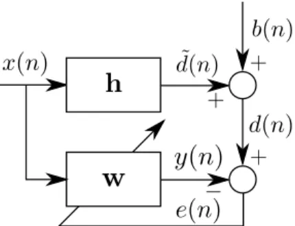
Figure 2.1: Supervised linear filtering model.

The supervised linear filtering problem consists of processing an input signal x(n)using a linear filter to produce an estimatey(n) of a desired signald(n)[1]. The linear filter is designed to minimize the estimation error e(n) :=d(n)−y(n)

(21)

by the convolution sum

y(n) =

N−1 X

k=0

w∗_kx(n−k) = wHx(n), (2.1)

where

w:= [w0, w1, . . . , wN−1]T∈CN

and

x(n) := [x(n), x(n−1), . . . , x(n−N + 1)]T _∈_CN

denote the filter coefficients vector and the input signal regression vector, respec-tively. The supervised linear filtering problem is illustrated in Figure 2.1.

The mean square error (MSE) is an attractive optimization criterion due to its mathematical tractability. Since the input signalx(n)is assumed to be WSS, it can be shown that the MSE curve is convex and has a unique global minimum [1]. In this context, we seek to minimize the MSE between y(n)andd(n), i.e. we aim at solving the following optimization problem:

min w

Eh_d₍_n₎₋_wH_x₍_n₎2i_, _(2.2)

where E_[_·_] _{denotes the statistical expectation operator.}

Let the objective function be defined asJw :=E h

d(n)−wHx(n)2 i

. The WH filter (Section A.1) provides the minimum mean square error (MMSE) solution to (2.2) by solving the ∇Jw = _∂∂J_wwH = 0 for w. On the other hand, the LMS

algorithm (Section A.2) solves (2.2) by using the stochastic gradient descent method. The Normalized Least Mean Square (NLMS) algorithm, reviewed in Section A.3, is a modified LMS which employs a variable step size factor. The reader is referred to Appendix A for more information on these classical filtering methods.

2.2 Supervised Multilinear Filtering

(22)

problem, multilinear (tensor) algebra prerequisites will be presented for conve-nience. Subsequently multilinear extensions of the linear filtering methods will be introduced.

2.2.1 Tensor Prerequisites

AnNth order tensor is essentially an element of a tensor product betweenN vector spaces [29]. Any Nth order tensor can be represented by a multidimen-sional coordinates array whenever the basis of the vector spaces V_n _{are set for}

n = 1, . . . , N. Hereafter the term “tensor” will refer to its multidimensional ar-ray representation, denoted by uppercase calligraphic letters, e.g. X ∈C×Nn=1In_,

where In := dim(Vn) for n = 1, . . . , N. The scalar tensor element indexed by

(i1, i2, . . . , iN) is denoted by [X]i1i2...iN := xi1i2...iN, where in ∈ {1, . . . , In} for

n = 1, . . . , N. Note that scalars can be regarded as 0th order tensors, vectors as 1st order tensors, and matrices as2nd order tensors. Other tensor definitions and operators will be defined next.

Definition 1 (Tensorization). Let Θ :CQNn=1In _→_C×N_n₌₁In denote the

tensoriza-tion operator, which transforms a vector v ∈ CQNn=1In into a tensor _Θ(_v₎ _∈

C×Nn=1In whose components are defined as

[Θ(v)]_i₁_i₂_...i_N := [v]_j, j :=i1+ N

X

n=2

(in−1) n−1 Y

v=1

Iv. (2.3)

For example, let N = 3, I1 = 2, I2 = 3, I3 = 4, and v ∈ CI1I2I3. The

tensorization of v isΘ(v)∈CI1×I2×I3 _{and its elements are given by}

[Θ(v)]i1i2i3 := [v]j, j := i1+ (i2−1)I1 + (i3−1)I1I2

for i1 ∈ {1,2}, i2 ∈ {1,2,3}, and i3 ∈ {1,2,3,4}.

Definition 2 (Vectorization). Let vec : C×Nn=1In _→ _CQN_n₌₁In denote the

vector-ization operator, which transforms a tensor X ∈C×Nn=1In into a vector vec₍_X₎_∈

CQNn=1In whose components are defined as

[vec(X)]j := [X]i1i2...iN, j := i1+

N

X

n=2

(in−1) n−1 Y

v=1

Iv. (2.4)

Definition 3(Tensor fiber [30]). Then-mode tensor fiber of anNth order tensor

X ∈ C×Nn=1In is defined as the vector formed by fixing every index but the _i

(23)

For instance, consider a third-order tensor U ∈ CI1×I2×I3_{. Its 1-, 2-, and} 3-mode fibers are given by

u·i2i3 ∈C I1_, ui1·i3 ∈C

I2_, ui1i2· ∈C

I3_,

where “·” denotes the varying index. Note that the vec(·) operator can be seen as the concatenation of the 1-mode fibers along the first dimension of a vector. Definition 4 (Tensor unfolding [30]). The n-mode unfolding of an Nth order tensor X ∈ C×Nn=1In is a matrix _X

(n) ∈ CIn×I1I2...In−1In+1...IN whose entries are

defined as

[X(n)]inj := [X]i1...iN, j := 1 +

N

X

u=1 u6=n

(iu−1) u−1 Y

v=1 v6=n

Iv.

For instance, the unfoldings ofU ∈CI1×I2×I3 _are

U₍₁₎ ∈CI1×I2I3_, U(2) ∈CI2×I1I3,

U(3) ∈CI3×I1I2.

Note that the n-mode matrix unfolding can be seen as the concatenation of the n-mode fibers along the matrix columns.

Definition 5 (Tensor concatenation [31]). The concatenation of T tensors Ut ∈

C×Nn=1In_{, t}_{= 1}_{, . . . , T,} along the ₍_M _{+ 1)}th dimension is denoted by

U =U1⊔M+1U2⊔M+1. . .⊔M+1UT ∈CI1×I2×...×IM×T,

where [U]i1i2...iMt= [Ut]i1i2...iM.

Definition 6 (Outer product). Consider an Nth order tensor U ∈C×Nn=1In and

an Mth order tensor V ∈ C×Mm=1Jm. The elements of the outer product T = U ◦ V ∈ CI1×...×IN×J1×...×JM are defined as

[T]i1...iNj1...jM :=ui1...iNvj1...jM, (2.5)

(24)

Definition 7 (Rank-1 tensor [30]). Any Nth order rank-1 tensor T ∈ C×Nn=1In

can be written as

T :=t1◦t2◦. . .◦tN, (2.6) where tn∈CIn for n = 1, . . . , N.

Definition 8 (Tensor rank). Tensor rank is defined as the minimum number of rank-1 components that exactly decomposes additively a tensor.

Definition 9 (Inner product [32]). Consider the tensors U ∈C×Nn=1In and _{V ∈}

C×Nn=1In with same dimensions. The inner product _hU_,_Vi is defined as

hU,Vi:=

I1

X

i1=1 I2

X

i2=1 . . .

IN

X

iN=1

ui1i2...iNv

∗

i1i2...iN, (2.7)

where (·)∗ _{denotes complex conjugation.}

Definition 10. The Frobenius norm of an Nth order tensor X ∈ C×Nn=1In is

defined as

kX k_F := v u u t I1 X

i1=1 I2

X

i2=1 . . .

IN

X

iN=1

|xi1i2...iN|

2

. (2.8)

The Frobenius norm (2.8) can be expressed in terms of an inner product

kX k_F =phX,X i.

Definition 11 (n-mode product [30]). The elements of the n-mode product be-tween an Nth order tensor X ∈ C×Nn=1In and a matrix _U _∈ _CJ×In is defined as

[X ×nU]_i₁_...i_n₋₁_ji_n₊₁_...i_N := In

X

in=1

xi1i2...iNujin, j ∈1, . . . , J, (2.9)

where “×n” denotes the n-mode product operator.

Definition 12. The elements of the {1, . . . , N}-mode product between an Nth order tensor X ∈ C×Nn=1In and a sequence of ₍_J

n × In)-dimensional matrices

{U(n)}N

n=1, denoted by Y =X ×1U(1). . .×N U(N)∈C×

N

n=1Jn, are defined as

[Y]_j₁_...j

N :=

I1

X

i1=1 . . .

IN

X

iN=1

xi1...iNuj1i1. . . ujNiN. (2.10)

It can be shown thatY(n), the n-mode unfolding of Y, is given by [30]

Y(n) =U(n)X(n)U⊗n T

(25)

where X(n) denotes the n-mode unfolding ofX, “⊗” the Kronecker product, and

U⊗n:= U(N)⊗. . .⊗U(n+1)⊗U(n−1)⊗. . .⊗U(1) (2.12) the Kronecker product of the matrices {U(j)}N

j=1 j6=n

in the decreasing order.

Definition 13(Multilinear operator [29]). An operatorf that mapsC₁_×_{. . .}_×C_N

onto C is said to be multilinear if _f₍_v₁_{, . . . ,}_v_N₎ is linear with respect to every

input vn for n = 1, . . . , N.

Definition 14 (Kronecker product). The elements of the Kronecker product v=N1_n₌_Nvn ∈C

QN

n=1In are given by

[v]j = N

Y

n=1

[vn]in, (2.13)

where vn ∈CIn for n= 1, . . . , N, and j :=i1 +PN_n₌₂(in−1)Qn_v₌₁−1Iv. Proposition 1. It follows that vec(T) = N1_n₌_Ntn ∈ C

QN

n=1In, where _T ₌ _t

1 ◦

t2◦. . .◦tN ∈C×

N

n=1 is a rank-1 tensor.

Proof. Let us substitute T =t1◦t2◦. . .◦tN into (2.4):

[vec(T)]j = [t1◦t2◦. . .◦tN]i1i2...iN

=

N

Y

n=1 [tn]in.

From Definition 2, we have that j = i1 + PN

n=2(in − 1)

Qn−1

v=1Iv. Therefore, vec(T) =tN ⊗tN−1⊗. . .⊗t1 holds according to Definition 14.

For example, leta= [a1, a2]T∈R2 and b= [b1, b2, b3]T∈R3. The Kronecker

product between these vectors is given by

a⊗b= [a1b1, a1b2, a1b3, a2b1, a2b2, a2b3]T.

The outer product between b and a, and its vectorization can be written as

b◦a=    b1 b2 b3   

a1, a2

=   

a1b1 a2b1

a1b2 a2b2

a1b3 a2b3   

(26)

and vec(b◦a) = [a1b1, a1b2, a1b3, a2b1, a2b2, a2b3]T, respectively.

Proposition 2. The inner product between an Nth order tensor U ∈ C×Nn=1In

and a rank-1 Nth order tensor V =v1◦v2◦. . .◦vN ∈C×

N

n=1In is given by

y(v1, . . . ,vN) :=hU,Vi =U ×1v1H×2vH2 . . .×N vHN ∈C, (2.14)

where (·)H _{denotes the Hermitian operator.}

Proof. From the definitions of the rank-1 tensor (2.6) and inner product (2.7), it follows that

y(v1, . . . ,vN) = hU,Vi

=hU,[v1◦v2. . .◦vN]i

=

I1

X

i1=1 I2

X

i2=1 . . .

IN

X

iN=1

ui1i2...iN[v1◦v2. . .◦vN]

∗

i1i2...iN

=

I1

X

i1=1 I2

X

i2=1 . . .

IN

X

iN=1

ui1i2...iN[v1]

∗

i1[v2]

∗

i2. . .[vN]

∗

iN. (2.15)

Equation (2.15) is recognized as a{1, . . . , N}-mode product (2.10), which is equal to (2.14).

Proposition 3. The inner product y(v1, . . . ,vN) = U ×1vH1 ×2vH2 . . .×N vHN is a multilinear operator.

Proof. Substituting equation (2.11) into y(v₁, . . . ,v_N)gives:

y(v1, . . . ,vN) = vHnxn n = 1, . . . , N, (2.16)

where xn = U(n)[v⊗n]∗. Note that y(v1, . . . ,vN) is linear with respect to the components of vn for n= 1, . . . , N, completing the proof.

Proposition 4. Let

X := [X(1)⊔M+1. . .⊔M+1X(K)]∈CN1×...×NM×K

denote the concatenation of K tensors with same dimensions along the(M + 1)th dimension. The{1, . . . , m−1, m+1, . . . , N}-mode product betweenX and{wH_j}M

(27)

for m = 1, . . . , M is given by

U(m) =X ×1w1H. . .×m−1wmH−1×m+1wmH+1. . .×M wHM (2.17)

=u(1)_m , . . . ,u_m(K)∈CNm×K_,

where u(mk) :=X(₍k_m)₎w⊗m ∈CNm, m∈ {1, . . . , M}. Proof. The elements of (2.17) are given by:

U(m) nm,k =

N1

X

n1=1 . . .

Nm−1

X

nm−1=1 Nm+1

X

nm+1=1 . . .

NM

X

nM=1

[X]n1...nMk[w1]

∗

n1. . .[wm−1]

∗

nm−1[wm+1]

∗

nm+1. . .[wM]

∗

nM

(2.18) fornm = 1, . . . , Nmandk= 1, . . . , K. From Definition 5, it follows that[X]n1n2...nMk =

[X(k)_]

n1n2...nM and that the elements of (2.18) become:

U(m) nm,k =

N1

X

n1=1 . . .

Nm−1

X

nm−1=1 Nm+1

X

nm+1=1 . . .

NM

X

nM=1

[X(k)]n1...nM[w1]

∗

n1. . .[wm−1]

∗

nm−1[wm+1]

∗

nm+1. . .[wM]

∗

nM,

From the equation above, we notice that the kth column of U(m) is given by the

{1, . . . , m−1, m+ 1, . . . , M}-mode product um(k) :=X(₍k_m)₎w⊗m.

2.2.2 Problem Formulation

Now let us introduce the multilinear generalization of the supervised linear filtering problem presented in the last Section. For simplicity’s sake, we consider rank-1 separable systems. Consider an Mth order separable FIR system whose coefficients vector is given by

h= 1 O

m=M

(28)

where hm ∈ CNm denotes itsmth order subsystem for m = 1, . . . , M. An input signal x(n) feeds the unknown system, producing

˜

d(n) = hHx(n)

=

N

X

k=1

[h]∗_k[x(n)]k

=

N1

X

k1=1 N2

X

k2=1 . . .

NM

X

kM=1

[h1]∗k1[h2]

∗

k2. . .[hM]

∗

kM[x(n)]k′, (2.20)

where k′ _:=_k

1+PMm=2(km−1)Qmv=1−1Nv. A separable FIR filter

w= 1 O

m=M

w_m ∈CN_, _(2.21)

where wm ∈ CNm is employed to identify h. This filter is fed by x(n) as well, yielding an output signal

y(n) =

N1

X

k1=1 N2

X

k2=1 . . .

NM

X

kM=1

[w1]∗k1[w2]

∗

k2. . .[wM]

∗

kM[x(n)]k′. (2.22)

From Proposition 1, hand ware vectorizations of the Mth order rank-1 tensors

H =h1◦. . .◦hM andW =w1◦. . .◦wM, respectively. The input regression vector can be regarded as the vectorization of X(n) := Θ[x(n)]∈C×Mm=1Nm_{. According}

to Proposition 2, equations (2.20) and (2.22) become

d(n) = X(n)×1hH1 . . .×M hHM

and

y(n) = X(n)×1wH1 . . .×M wHM,

respectively. These filtering operations are multilinear with respect to each sub-system (filter) as shown in Proposition 3. In view of this, equations (2.20) and (2.22) are hereafter referred to as multilinear filtering.

Definition 15(Multilinear filtering). Consider anMth order input tensorX(n)∈ C×Mm=1Nm and a rank-1 tensor filter_W ₌_w

(29)

This filter produces a complex valued output signal

y(n) = hX(n),Wi

=X(n)×1wH1 ×2wH2 . . .×M wHM. (2.23)

The supervised multilinear filtering approach to system identification consists of approximating a distorted desired signal d(n) = ˜d(n) +b(n) using a rank-1 tensor filter W, where b(n) is a zero mean and unit variance additive white Gaussian measurement noise component uncorrelated to d˜(n) and x(n). The supervised multilinear filtering can be expressed as the following optimization problem:

min w1,...,wM

Ehd(n)− X(n)×₁w₁H. . .×M wHM

2

i

. (2.24)

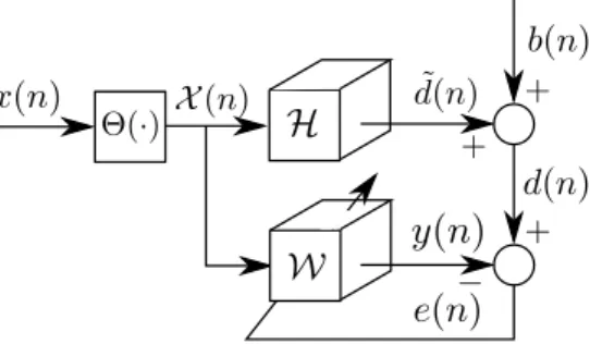
The multilinear system identification model is illustrated in Figure 2.2. Note that when M = 1 (not separable case), the supervised multilinear filtering problem reduces to its linear counterpart.

Figure 2.2: Supervised multilinear system identification model.

We have remarked a link between Kronecker products and cascade filters, and we will show that Kronecker factorization leads to a system factorization in terms of sparse subsystems, which we refer to as extended subsystems. We propose in the following the Extended Subsystem Factorization Theorem: Theorem 1(Extended Subsystem Factorization). AnyMth order separable FIR system whose coefficients vector decomposes intoh=N1_m₌_Mhmcan be expressed as

h= ˜h₁∗h˜₂∗. . .∗h˜_M, (2.25) where “∗” denotes discrete-time convolution,_h˜_m _∈C(Nm−1)Ψm+1 denotes the mth

order extended subsystem, and Ψm =

Qm−1

(30)

subsystems are given by

[˜hm]nm =

  

[hm](nm−1)/Ψm , if (nm−1) mod Ψm = 0

0 , otherwise , (2.26)

for nm = 1, . . . , Nm.

Proof. From Definition 14, it follows that the (n + 1)th element of h can be written as:

[h]n+1 = [h1]n1+1[h2]n2+1. . .[hM]nM+1, (2.27)

wheren =n1+PM_m₌₂nmQ_vm₌₁−1Nv fornm ∈ {0, . . . , Nm−1}and m= 1, . . . , M. Let us study the separability effect on the Z-transform ofh, which is denoted by H(z):

H(z) =

N−1 X

n=0

[h]n+1z−n

=

N1−1

X

n1=0 N2−1

X

n2=0 . . .

NM−1

X

nm=0

[h₁]n1+1[h2]n2+1. . .[hM]nM+1z

−(n1+PMm=2nmQm_v₌₁−1Nv)

=

N1−1

X

n1=0

[h1]n1+1z

−n1

! _N₂₋₁ X

n2=0

[h2]n2+1z

−n2N1

!

. . .

NM−1

X

nM=0

[hM]nM+1z

−nMQMv=1−1Nv

!

= ˜H1(z) ˜H2(z). . .H˜M(z). (2.28)

The term H˜m(z) denotes the Z-transform of the mth extended subfilter. It can be expressed as:

˜

Hm(z) = [hm]1+ [hm]2z−Ψm+ [hm]3z−2Ψm+. . .+ [hm]Nmz

−(Nm−1)Ψm_. _(2.29)

Note that the elements ofH˜m(z)are nonzero when the exponent ofzis a multiple of Ψm. In view of this, the inverse Z-transform of (2.29) is given by:

[˜hm]nm =

  

[hm](nm−1)/Ψm , if (nm−1)mod Ψm = 0

0 , otherwise , (2.30)

fornm = 1, . . . , Nm. Considering (2.30), the inverse Z-transform of (2.28) is given by h= ˜h1∗h˜2∗. . .∗h˜M.

To illustrate this result, let us consider the following example. Leth =h1⊗

(31)

and I3 = 4. According to Theorem 1, h can be convolutionaly decomposed into

h = ˜h1∗h˜2∗h˜3, where ˜

h1 = h

h(1)₁ h(1)₂ iT

1×2, ˜

h2 = h

h(2)₁ 0 h(2)₂ 0 h(2)₃

iT

1×5, ˜

h3 = h

h(3)₁ 0 0 0 0 0 h(3)₂ 0 0 0 0 0 h(3)₃ 0 0 0 0 0 h(3)₄

iT

1×19.

andh(nm) := [hm]n. This factorization is depicted in Figure 2.3. We notice that the extended subsystems h˜m are oversampled/sparse versions of their correspondent subfilter hm.

Figure 2.3: Extended subsystem factorization example.

In the next Section, we will introduce a method for estimating the extended subfilters using WH filters.

2.2.3 Separable Wiener-Hopf Algorithm

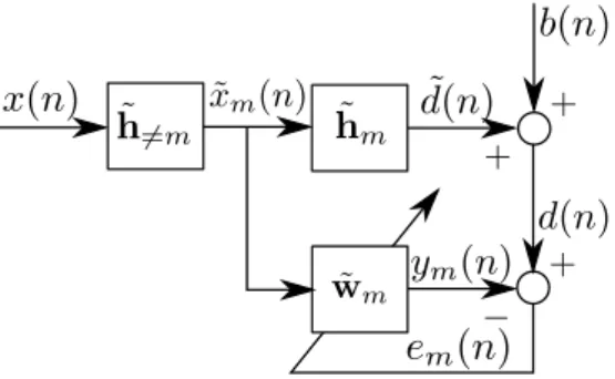
The Separable Wiener-Hopf (SepWH) algorithm consists of dividing the mul-tilinear filtering problem (2.24) into M independent linear subproblems. This division is carried out by factorizing the unknown FIR system h in terms of its extended subsystemsh˜mand individually identifying them usingw˜m, the WH fil-ter presented in Appendix A. Affil-terwards, the system identification is completed by computing w= ˜w1∗. . .∗w˜M. Since the solution of a linear subproblem does not depend on the other solutions, they are said to be independent.

The linear subproblem corresponding to the mth extended subfilter is given by

min ˜

wm

Ehd(n)−w˜_mHx˜_m(n)2 i

, m∈ {1, . . . , M}, (2.31) where it is supposed that ˜xm(n) := x(n)∗h˜6=m, the prefiltered regression vector, is observable, and h˜6=m := ∗Mk=1

k6=m

˜

(32)

illustrated in Figure 2.4. The SepWH has a computational complexity given by

O((NM −1)ΨM + 1)3

since it inverts a [(NM−1)ΨM+ 1×(NM−1)ΨM+ 1] -dimensional autocorrelation matrix.

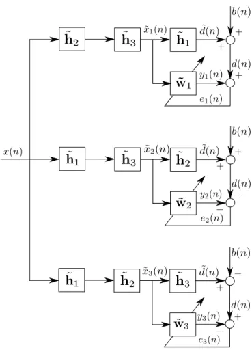
Figure 2.4: Separable Wiener-Hopf algorithm structure.

Let us illustrate the SepWH algorithm structure by using an example. Con-sider a third-order separable FIR system whose coefficients vector is given by h =h3⊗h2⊗h1 ∈CI1I2I3, where h1 ∈ CI1, h2 ∈CI2, h3 ∈CI3, I1 = 2, I2 = 3,

and I3 = 4. The estimation ofw˜1, w˜2, and w˜3 is illustrated in Figures 2.5. The

SepWH algorithm is summarized in Algorithm 1. Algorithm 1 Separable Wiener-Hopf algorithm

1: _procedure SepWH(x(n), _h₁, . . . ,_h_M) 2: _h ←_h₁∗_h₂∗. . .∗_h_M

3: Calculate h˜_m using Eq. (2.26) form= 1, . . . , M 4: _for m= 1, . . . , M _do

5: for t= 0, . . . , T −1 do

6: h˜₆₌_m ← ∗M

k=1 k6=m

˜

hk

7: x˜_m(n−t)←x(n−t)∗h₆₌_m 8: d(n−t)←_hH_x˜(n) +b(n−t) 9: _R_x_˜ ←(1/T)_x(n−t)_x(n−t)H 10: p_d_x_˜ ←(1/T)d∗(n−t)x(n−t)

11: _w˜_m ←_R−1

˜

x pdx˜

12: _{end for}

13: end for

14: _w←_w˜₁∗_w˜₂∗. . ._w˜_M 15: _{end procedure}

2.2.4 Tensor Wiener-Hopf Algorithm

(33)

(34)

alternating optimization approach [26, 33] has demonstrated to solve the global nonlinear problem in terms ofM smaller linear problems. It consists of updating the mth mode subfilter each time by solving (2.24) for wm, while {wj}Mj=1,j6=m remain fixed, m = 1, . . . , M, conditioned on the previous updates of the other subfilters. In this sense, (2.24) can be divided inMinterdependent linear subprob-lems using them-mode unfolding equation (2.11). This allows us to represent the multilinear filtering (2.23) in terms ofM different but equivalent linear filtering:

y(n) =wH₁X₍₁₎(n) (wM ⊗wM−1⊗. . .⊗w2)∗ =wH1u1(n), =wH₂X(2)(n) (wM ⊗wM−1⊗. . .⊗w1)∗ =wH2u2(n),

... = ...

=wH_MX(M)(n) (wM−1 ⊗wM−2⊗. . .⊗w1)∗ =wHMuM(n),

where

um(n) = X(m)(n)w⊗m ∈CNm, m∈ {1, . . . , M}. (2.32)

Substituting the equations above in (2.24) gives

min wm

Ehd(n)−wH_mum(n)

2

i

, m ∈ {1, . . . , M}. (2.33)

The solution of (2.33) is given by the Wiener-Hopf filter (A.3):

wm_opt =R−_m1pm, m∈ {1, . . . , M}, (2.34)

where

Rm :=E

um(n)um(n)H

=Eh_X₍_m₎₍_n₎_w⊗m _w⊗mH _X₍_m₎₍_n₎Hi _(2.35)

and

pm :=E[um(n)d∗(n)]

=E_X₍_m₎₍_n₎_w⊗m_d∗₍_n₎ _(2.36)

(35)

We propose the TWH algorithm, which is based on the alternating least squares (ALS) method to estimate w_optm by data averaging in the time interval T. Let

X = [X(n)⊔M+1. . .⊔M+1X(n−T + 1)]∈CN1×...×NM×T

denote the concatenation of T time snapshots of X(n) along the (M + 1)th dimension. Let U(m) ∈ CNm×T denote the {1, . . . , m−1, m+ 1, . . . , N}-mode

product between X and {wH

j}Mj=1,j6=m for m= 1, . . . , M:

U(m)=X ×1wH1 . . .×m−1wmH−1 ×m+1wmH+1. . .×M wHM. (2.37)

From Proposition 4, it follows that U(m) = [u_m(n), . . . ,u_m(n−T + 1)]. There-fore the sample estimates of R_m and p_m are given by:

ˆ

Rm =

1

TU

(m)_U(m)H

, (2.38)

ˆ

pm =

1

TU

(m)_d∗_, _(2.39)

where d = [d(n), d(n−1), . . . , d(n−T + 1)]T ∈ CT_{. Now the} _{mth order}

sub-filter updating rule (2.34) becomes wˆ_optm = ˆR−_m1pˆm. At the end of the subfilter estimation stage, the global filter is computed aswˆ =N1_m₌_Mwˆm. The subfilters are estimated in an alternate fashion until convergence, which is attained when the relative system mismatch, defined as kh−wˆk2

2/khk22, between two

consec-utive iterations is smaller than a threshold ε. This procedure is summarized in Algorithm 2.

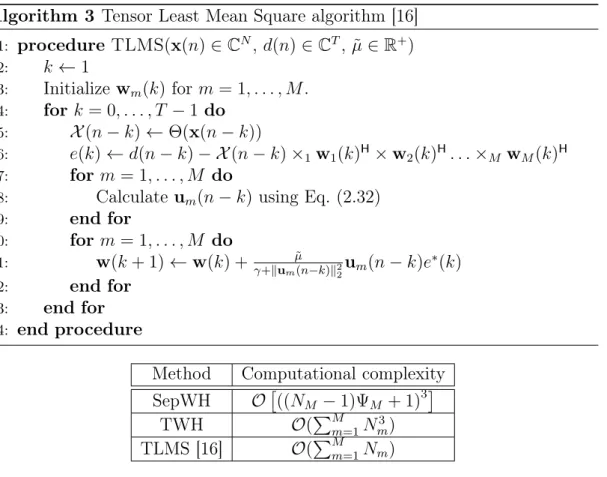
The TWH algorithm has a computational complexity ofOPM_m₌₁N3 m

. Such an alternating minimization procedure has a monotonic convergence [34]. It is worth mentioning that an analytical convergence analysis of this algorithm is a challenging research topic which is under investigation.

2.2.5 Tensor LMS Algorithm [16]

As in the linear filtering scenario, the optimization problems (2.24) can be solved using a stochastic gradient approach. The gradient of the instantaneous objective function Jwm(n) = E

h

d(n)−wH mum(n)

2

i

corresponding to the mth filtering mode is given by

ˆ

∇Jwm(n) =−um(n)um(n)

H_w

(36)

Algorithm 2 Tensor Wiener-Hopf algorithm procedure TWH(X, s,ε)

k ←1

Initialize e(k), wm(k), m= 1, . . . , M. repeat

for m= 1, . . . , M do

Calculate U(m)(k)using Equation (2.37)

ˆ

R_m ←(1/T)U(m)U(m)H

ˆ

pm ←(1/T)U(m)s∗

ˆ

wm(k+ 1)←Rˆ−m1pˆm end for

k←k+ 1

y(k)← X ×1wˆ1(k)H. . .×M wˆM(k)H e(k) = ks−y(k)k2

2/T

until |e(k)−e(k−1)|< ε end procedure

In [16], M. Rupp and S. Schwarz proposed the Tensor Least Mean Square (TLMS) update rule for the mth order filter using a variable step size µ(n):

wm(n+ 1) =wm(n)−µ(n) ˆ∇Jwm(n)

=wm(n)−µ(n)

−um(n)um(n)Hwm+um(n)d∗(n)

=wm(n) +µ(n)um(n)

w_mHum(n)−d(n)

∗

=w_m(n) +µ(n)u_m(n)e∗_m(n). (2.41)

The authors indicated that TLMS converges for M = 2 if

0< µ(n)< 2

ku1(n)k22 +ku2(n)k22

. (2.42)

In this work, we have used µ(n) = PM µ˜

m=1kum(n)k22 for some values of µ˜ such that TLMS attained convergence. This algorithm could be named “Tensor Normalized Least Square” due to the step size normalization w.r.t.um(n),m= 1, . . . , M, but we preferred to keep the original acronym. Each TLMS iteration, which consists of updating all M subfilters, has computational complexityOPM_m₌₁Nm

. An-alytical study of convergence of the TLMS algorithm remains an open research problem. TLMS is summarized in Algorithm 3. In line 11, γ ∈ R+ _{is a constant}

(37)

Algorithm 3 Tensor Least Mean Square algorithm [16]

1: _procedure TLMS(x(n)∈CN_, _d₍_n₎_∈CT_,_µ_˜_∈R+₎

2: k ←1

3: Initialize _w_m(k) for m= 1, . . . , M. 4: _for k = 0, . . . , T −1 _do

5: X(n−k)←Θ(x(n−k))

6: e(k)←d(n−k)− X(n−k)×₁_w₁(k)H×_w₂(k)H. . .×_M _w_M(k)H 7: _for m = 1, . . . , M _do

8: Calculate u_m(n−k) using Eq. (2.32)

9: _{end for}

10: _for m = 1, . . . , M _do

11: w(k+ 1)←w(k) + µ˜

γ+kum(n−k)k22um(n−k)e

∗₍_k₎

12: end for

13: end for 14: _{end procedure}

Method Computational complexity SepWH O((NM −1)ΨM + 1)3

TWH O(PM_m₌₁N3 m) TLMS [16] O(PM_m₌₁Nm)

Table 2.1: Computational complexity of the SepWH, TWH, and TLMS algo-rithms.

(38)

Chapter 3 Supervised Identification of

Multilinear Systems

In this chapter, computer simulations were conducted to assess the perfor-mance of the proposed filtering methods in the system identification context. The system model is described in Section 3.1, the obtained results are shown in Section 3.2, next they are discussed in Section 3.3.

3.1 System Model

Figure 3.1: Supervised system identification model.

(39)

using system identification techniques.

Consider an unknown system modeled by an Nth order real FIR system whose coefficients vector h∈RN _is_M_{th order separable, i.e.}

h=hM ⊗hM−1 ⊗. . .⊗h1, (3.1)

where hm ∈ RNm is the coefficients vector corresponding to the mth order sub-system for m = 1, . . . , M, and QM_m₌₁Nm = N. An Nth order real FIR filter whose coefficients vectorw=wM⊗wM−1⊗. . .⊗w1 isMth order separable was

placed parallel to the unknown system to identify its model, as illustrated in Fig-ure 3.1. Both systems were excited by a zero mean and unit variance signal x(n). The unknown system produced a distorted desired signal d(n) = ˜d(n) +b(n), where d˜(n) := hT_x₍_n₎_, _x₍_n_{) := [}_x₍_n₎_{, x}₍_n ₋₁₎_{, . . . , x}₍_n ₋_N _{+ 1)]}T_{, and} _b₍_n₎ denotes a zero mean and unit variance additive white Gaussian measurement noise component uncorrelated with d˜(n) and x(n).

3.2 Numerical Results

Monte Carlo (MC) simulations ofR = 100independent realizations were con-ducted to calculate the figures of merit of the NLMS, WH, SepWH, TLMS, and TWH methods. Tensors operations were computed using the Tensorlab toolbox [36]. Each figure of merit was expressed as a function of the input sample size K, the filter lengthN, and the SNR, which is defined as

SNR:= E

h

|d˜(n)|2i E_[_|_b₍_n₎_|2_] .

In this chapter, the mean relative system mismatch

ρ:= 1

R R

X

r=1

kh(r)−w(r)k2 2

kh(r)_k2 2

,

and the number of floating-points operations per second (FLOPS) demanded to attain convergence were chosen as figures of merit. The former allows to assess the system identification accuracy, whereas the latter provides the algorithm overall computational cost. The superscript (·)(r) _{denotes the}_{rth MC run. The number}

(40)

The coefficients of all (sub)filters were randomly initialized in all iterative algorithms. The step size of the LMS-based algorithms was set toµ= 10−2_{. The}

autocorrelation matrix and the cross-correlation vector of the WH filter were es-timated directly from data. Convergence in TWH was attained when the relative system mismatch difference between two consecutive ALS steps was smaller than ε = 10−3_{. To check convergence, TLMS compares the relative system mismatch}

at the current iteration with that of 2000 past iterations. This is because the TLMS mean system mismatch difference in a few consecutive iterations may be too small due to slow convergence with a small step size factor.

In the first simulation scenario, the coefficients vector of the unknown system (3.1) was 3rd order separable (M = 3). Its subsystems h1 ∈ RN1, h2 ∈ RN2,

and h3 ∈ RN3 were randomly generated accordingly to a zero mean Gaussian

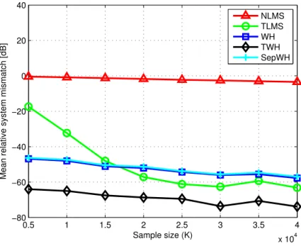
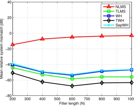
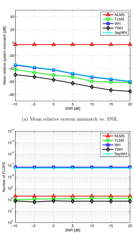
distribution with identity covariance matrix and null mean vector. The influence of the input sample size K, the filter length N, and the SNR on the methods performance was assessed in three simulations where one parameter varied while the others remained fixed. In Figures 3.2, 3.3, and 3.4, the figures of merit are depicted as functions of K, N, and SNR, respectively.

Another simulation was conducted to analyze the effect of the step size fac-tor on the TLMS performance and to compare it to the TWH algorithm. The obtained learning curves for a step size µ ∈ {10−1_,₁₀−2_,₁₀−3_} _{are depicted in}

Figure 3.6 and the corresponding results are shown at Table 3.3.

In the second simulation scenario, the influence of the separability order M on the TWH method performance was studied. In order to consistently compare this influence, it was necessary to consider a system whose coefficients vector h was equivalently separable across different separability orders, i.e.

h= 1 O

m=M h_m =

1 O

j=J

h_j, ∀M, J ∈Z+_. _(3.2)

Exponential systems fulfills the condition (3.2) and were considered in this sce-nario. More specifically, the coefficients of h were defined as

[h]n:= exp

−0.1(n−1)

N

forn= 1, . . . , N (3.3)

The reader is referred to Appendix B for more information on the exponential system separability.

(41)

SNR forM = 2,3, . . . ,6and plotted in Figures 3.7, and 3.10, respectively. When analyzing the effect of the system length, it was necessary to assure that the system length remained constant across different values of M, i.e. QM_m₌₁Nm =

QJ

j=1Nj, ∀M, J ∈ Z+. In view of this, two sets of subsystem dimensions were considered. In the first set (Table 3.1), the subsystem dimensions were chosen to be similar, whereas, in the second set (Table 3.2), there was a subfilter with a larger dimension. TWH performance is plotted as a function of the system length N in Figures 3.9 and 3.8 for dimensions sets at Table 3.1 and Table 3.2, respectively.

N M

2 3 4 5 6

128 8×16 8×4×4 4×4×4×2 2×2×2×4×4 2×2×2×2×2×4

256 16×16 8×8×4 4×4×4×4 2×2×4×4×4 2×2×2×2×4×4

512 16×32 8×8×8 8×4×4×4 2×4×4×4×4 2×2×2×4×4×4

1024 32×32 8×8×16 8×8×4×4 2×4×4×4×8 2×2×2×4×4×8

Table 3.1: Similar subsystem dimensions.

N M

2 3 4 5 6

200 20×20 2×10×20 2×2×10×10 2×2×2×5×10 2×2×2×2×5×5

600 20×30 2×10×30 2×2×10×15 2×2×2×5×15 2×2×2×3×5×5

800 20×40 2×10×40 2×2×10×20 2×2×2×5×20 2×2×2×4×5×5

1000 20×50 2×10×50 2×2×10×25 2×2×2×5×25 2×2×2×5×5×5

Table 3.2: Different subsystem dimensions.

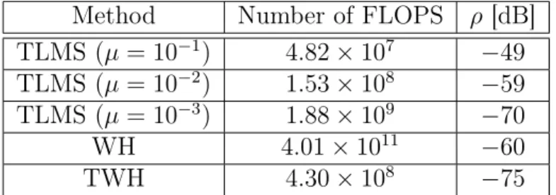
Method Number of FLOPS ρ [dB] TLMS (µ= 10−1₎ ₄_.₈₂_×₁₀7 ₋₄₉

TLMS (µ= 10−2₎ ₁_.₅₃_×₁₀8 ₋₅₉

TLMS (µ= 10−3₎ ₁_.₈₈_×₁₀9 ₋₇₀

WH 4.01×1011 ₋₆₀

TWH 4.30×108 ₋₇₅

(42)

0.5 1 1.5 2 2.5 3 3.5 4 x 104 −80

−60 −40 −20 0 20 40

Sample size (K)

Mean relative system mismatch [dB]

NLMS TLMS WH TWH SepWH

(a) Mean relative system mismatch vs. Sample size.

0.5 1 1.5 2 2.5 3 3.5 4

x 104 106

107 108 109 1010 1011 1012 1013 1014

Sample size (K)

Number of FLOPS

(b) Number of FLOPS vs. Sample size.

(43)

200 300 400 500 600 700 800 900 1000 −80

−60 −40 −20 0 20 40

Filter length (N)

(a) Mean relative system mismatch vs. Filter length.

200 300 400 500 600 700 800 900 1000

106 107 108 109 1010 1011 1012 1013 1014

Filter length (N)

Number of FLOPS

(b) Number of FLOPS vs. Filter length.

(44)

−10 −5 0 5 10 15 20 −80

−60 −40 −20 0 20 40

SNR [dB]

(a) Mean relative system mismatch vs. SNR.

−10 −5 0 5 10 15 20

106 107 108 109 1010 1011 1012 1013 1014

SNR [dB]

Number of FLOPS

(b) Number of FLOPS vs. SNR.

(45)

0 0.5 1 1.5 2 2.5 3 3.5

x 104 10−4

10−3 10−2 10−1 100 101 102 103

Iterations

MSE

Figure 3.5: MSE performance for µ= 10−2_,_K _{= 35}_.₀₀₀ _samples,_N _{= 1000}_{, and}

SNR = 30dB.

0 0.5 1 1.5 2 2.5 3

x 105 −80

−70 −60 −50 −40 −30 −20 −10 0 10

Iterations

TLMS (µ=0.1) TLMS (µ=0.01) TLMS (µ=0.001) WH

TWH

µ=0.01 µ=0.1

µ=0.001

(46)

0.5 1 1.5 2 2.5 3 3.5 4 x 104 −68

−66 −64 −62 −60 −58 −56 −54 −52

Sample size (K)

M=2 M=3 M=4 M=5 M=6

(a) Mean relative system mismatch vs. Sample size.

1 2 3 4 5 6 7 8

106 107 108 109

Sample size (K)

Number of FLOPS

M=2 M=3 M=4 M=5 M=6

(47)

0 200 400 600 800 1000 1200 −70

−68 −66 −64 −62 −60 −58 −56 −54 −52 −50

Filter length (N)

M=2 M=3 M=4 M=5 M=6

0 200 400 600 800 1000 1200

106 107 108 109 1010 1011

Filter length (N)

Number of FLOPS

M=2 M=3 M=4 M=5 M=6

(48)

400 500 600 700 800 900 1000 −70

−68 −66 −64 −62 −60 −58 −56 −54 −52 −50

Filter length (N)

M=2 M=3 M=4 M=5 M=6

400 500 600 700 800 900 1000

106 107 108 109 1010 1011

Filter length (N)

Number of FLOPS

M=2 M=3 M=4 M=5 M=6

(49)

−10 −5 0 5 10 15 20 −75

−70 −65 −60 −55 −50 −45 −40

SNR [dB]

M=2 M=3 M=4 M=5 M=6

(a) Mean relative system mismatch vs. SNR.

−10 −5 0 5 10 15 20

107 108 109 1010

SNR [dB]

Number of FLOPS

M=2 M=3 M=4 M=5 M=6

(50)

3.3 Discussion

The NLMS algorithm performed poorly in estimating the parameters of the unknown systems, as depicted in Figures 3.2a, 3.4a, and 3.3a. Since the parameter space was very large, much more iterations would be necessary to attain conver-gence. The effect of the filter length N on NLMS performance is clear on Figure 3.3a. Smaller systems demanded less iterations, allowing the NLMS algorithm to achieve mismatch levels as low as −17dB. Although this algorithm provides the worst parameter estimation accuracy, it has a small overall computational complexity.

Although the SepWH method exploited the system separability, it did not present any advantages with respect to the WH filter. As can be seen in Figures 3.2, 3.3, and 3.4, this method offered the same parameter estimation accuracy and computational complexity as its classic counterpart. In fact, the optimiza-tion stages in this method consists of independent least-squares subproblems, which do not incorporate the multilinear interdependence on their solution as TLMS and TWH do. Furthermore, the oversampling of the extended subsystems augmented their dimension, increasing the overall computational complexity and counterpoising the separability exploitation.

The TLMS algorithm provided better estimation accuracy than the methods discussed above in specific situations. As can be seen in Figure 3.2a, it started to be more accurate than the WH filter after the sample size was greater than 20.000. Since the alternating optimization approach employed by TLMS properly exploited the subfilter interdependency, it provided better accuracy than the WH filter. Figures 3.2b, 3.4b, and 3.3b showed that its computational complexity was similar to that of NLMS. The results shown in Figure 3.6 and Table 3.3 show that, to attain a system mismatch as low as −70dB, it is necessary to use small step size factors. This restriction consequently demands a massive number of FLOPS from TLMS, whereas TWH requires less FLOPS to provide an even more accurate parameter estimation.

(51)

it demanded more samples to achieve convergence. In Figure 3.3a, the TWH algorithm provided the best accuracy for all filter lengths.

In a first moment, it is surprising to see that any method performed better than the WH filter, which provides the MMSE estimate. However, it is important to stress that the results presented in Figures 3.2, 3.3, and 3.4 did not compare the MSE, but mean relative system mismatch. In fact, both linear and multilinear filtering methods are bounded by the MMSE, as observed in Figure 3.5. While 2nd order separable systems have a lower-bound on relative system mismatch estimation, as shown in [16], today there are similar no theoretical bounds for higher-order systems for the best of our knowledge.

It is interesting to remark that although TWH is a batch-based filtering method, it has an overall computational cost similar to that of adaptive filtering methods, as shown in Figures 3.2b, 3.3b, and 3.4b. The computational complex-ity of a TWH iteration is indeed superior than that of TLMS, as it can be seen in Table 2.1. However, TWH converges fastly, yielding a reduced overall com-putational complexity, whereas TLMS demands a large of amount of FLOPS to attain convergence in such large-scale scenarios.

The simulation in the second scenario showed that the separability order has an important influence on the multilinear filtering methods performance. Higher separability order leads to better accuracy and lower computational costs, as can be seen in Figures 3.7, 3.8, 3.9, and 3.10. Since the subfilters length decreases with M, the computational cost associated with the estimation of each subfilter is lower. Consequently, the overall computational cost reduces withM. Addition-ally, these figures show that there is a limit on the accuracy gain. Therefore, the system separability order offers an estimation accuracy / computational cost.

The results concerning the subfilter dimensions indicates that it determines the accuracy gain and the computational costs of multilinear filtering methods. When the system was partitioned into subsystems with similar dimensions, the performance depicted in Figure 3.8 was observed. By contrast, systems decom-posed into subsystems whose dimensions differed from those of the other sub-systems presented the performance described in Figure 3.9. We have observed that similar partitioning offered a −2dB gain forM = 3,4,5with respect to the other partitioning, as can be seen in Figure 3.9. Furthermore, similar partitioning presented lower computational costs in the same M interval.

(52)

(53)

Chapter 4 Beamforming for Multilinear

Antenna Arrays

In this chapter, we present the results obtained from computer simulations conducted to assess the performance of the TWH algorithm. The proposed sys-tem model was first introduced in [38], and it is described in Section 4.1. The obtained results from the simulations are shown in Section 4.2, next they are discussed in Section 4.3.

4.1 System Model

An antenna array consists of multiple sensors placed in different locations but physically connected that are used to process the impinging signals using a spatial filter. This filter is abeamformer when it is employed to enhance a signal of interest (SOI) arriving from a certain direction while attenuating any possible interfering signal [39].

Let us consider a translation invariant array ofN isotropic antennas located atp˜_n ∈R3×1_for_n_{= 1}_{, . . . , N}_{. It is formed by}_N₁ _{reference sensors located at}_p(1)_n

1 forn1 = 1, . . . , N1. Then1th reference sensor is translatedM−1times by means

of the translation vectorsp(2)n2, . . . ,p

(M)

nM , yielding the following decomposition for

the nth global sensor location vector [40]

˜

pn=p(1)n1 +p

(2)

n2 +. . .+p

(M)

nM , (4.1)

(54)

Figure 4.1: A 4×2×2volumetric array decomposed into three equivalent forms. Reference subarrays are indexed by m= 1, whereas m >1 refers to translation.

Now consider that R narrowband source signals with complex amplitudes sr(k) impinge on the global array from directions

dr = [sinθrcosφr,sinθrsinφr,cosθr]T,

where θr and φr denote the elevation and azimuth angles, respectively, for r =

1, . . . , R. The sources are assumed to be in the far-field and uncorrelated. It is also assumed that there are no reflection components. The received signals at instant k can be written as:

x(k) =

R

X

r=1

a(d_r)sr(k) +b(k)∈CN×1, (4.2)

where

a(dr) =

   

eω_cp˜T

1dr

... eω

cp˜TNdr

   =     

eω cp

(1)T

1 dr. . . eω_cp(M)

T

1 dr

... eωcp

(1)T

N₁ dr

. . . eωcp

(M)T

NM dr

     (4.3)

is the array steering separable vector, b(k) ∈ CN×1 _{is the additive zero-mean}

complex white Gaussian noise vector with covariance matrix equal to σ2_I, _ω

is the wave frequency, and c the velocity of propagation in the medium. Here we assume that the array interelement spacing d is smaller than λ/2, where λ := 2πc/ω denotes the wavelength. Equation (4.3) can be expressed as

a(dr) = a(M)(dr)⊗. . .⊗a(1)(dr)∈C

QM

m=1Nm_, _(4.4)

where a(m)(d_r) =

eω cp

(m)T

1 dr, . . . , eωcp

(m)T

Nm dr

T

(55)

vector associated with the mth order translation vector p(nmm),nm ∈ {1, . . . , Nm}.

Indeed, (4.4) is a vectorization of a rank-1 array steering tensor defined as

A(dr) =a(1)(dr)◦. . .◦a(M)(dr)∈C×

M

m=1Nm_. _(4.5)

In view of this, the received signals (4.2) can be expressed as a linear combination of R rank-1 tensors:

X(k) =

R

X

r=1

A(dr)sr(k) +B(k), (4.6)

where B(k) = Θ(b(k)) ∈ C×Mm=1Nm _{is the tensorized form of the noise vector}

b(k). A rank-1 tensor filterW ∈C×Mm=1Nm _{is proposed to perform beamforming}

exploiting the multilinear separable array structure [38].

4.2 Numerical Results

Computer experiments were conducted in order to assess the SOI estimation performance and the computational complexity of the tensor beamformer. In this context, R = 3 QPSK signals with unitary variance, carrying K symbols and arriving from the directions displayed at Table 4.1 were considered. The signal corresponding to r = 1 was set as SOI.

Source Azimuth [rad] Elevation [rad]

r= 1 (SOI) π/3 −π/4

r = 2 π/6 π/3

r = 3 π/4 −π/6

Table 4.1: Direction of arrival of the QPSK sources.

The classical WH filter (A.3) was used as benchmark method. The autocor-relation matrix and the cross-corautocor-relation vector of the WH filter were estimated directly from data. The convergence threshold of TWH was set to ε = 10−3_.

The mean performance indices were calculated by averaging the results obtained in J = 100 MC realizations. The SOI estimation performance was evaluated in terms of the MSE measure, defined as

MSE= 1

J J

X

j=1 1

Kks

(56)

where

s= [sSOI(k), sSOI(k−1), . . . , sSOI(k−K+ 1)]T∈CK

and ˆs(j) ∈ CK _{is the decided symbols vector whose} _{kth entry is the symbol} de-cided from the statistic hX(k),Wi. As in the previous chapter, the number of FLOPS demanded by each method was computed using the Lightspeed MAT-LAB toolbox [37], and the Tensorlab toolbox [36] was used to implement the tensor operations of the multilinear methods.

Three simulation scenarios were considered. In the first scenario, the perfor-mance indices were calculated by varying the sample size K, as illustrated in Figure 4.3. In this case, the global array consisted of N = 128 sensors. In the second scenario, the performance indices were calculated by varying the number N of sensors of the global array for K = 5000samples, as depicted in Figure 4.4. In the third scenario, the performance was assessed by varying the SNR, while keeping the sample size and the number of sensors fixed, as illustrated in Fig-ure 4.5. In all scenarios, the global array was formed by translating a reference uniform rectangular array along the x-axis, as illustrated in Figure 4.2.

(57)

4.3 Discussion

(58)

1000 2000 3000 4000 5000 6000 7000 8000 9000 10000 −40

−39 −38 −37 −36 −35 −34 −33 −32 −31 −30

Number of samples (K)

MSE [dB]

TWH (M=2) TWH (M=3) TWH (M=4) WH

(a) MSE vs. Sample size.

1000 2000 3000 4000 5000 6000 7000 8000 9000 10000 0

0.5 1 1.5 2 2.5 3 3.5x 10

8

Number of samples (K)

Number of FLOPS

(59)

0 100 200 300 400 500 −44

−42 −40 −38 −36 −34 −32 −30 −28 −26

Number of sensors (N)

MSE [dB]

(a) MSE vs. Number of sensors.

0 100 200 300 400 500

0 0.5 1 1.5 2 2.5

x 109

Number of sensors (N)

Number of FLOPS

(b) Number of FLOPS vs. Number of sensors.

(60)

0 5 10 15 20 25 30 −70

−60 −50 −40 −30 −20 −10

SNR [dB]

MSE [dB]

(a) MSE vs. SNR.

0 5 10 15 20 25 30

0.5 1 1.5 2 2.5

3x 10

8

SNR [dB]

Number of FLOPS

(61)

Chapter 5 Conclusion

In this thesis, we have proposed a computationally efficient tensor method for large-scale multilinear filtering problems. In the context of supervised system identification, we have shown that separable FIR filters admit a factorization in terms of its subfilters, which leads to a multilinear filtering structure. This multilinearity calls for a tensor formulation that leads to the separate estimation of each subfilter, allowing the computational complexity reduction and accurate system identification. In the context of array processing, we have proposed a multilinear model for translation invariant arrays that allowed us to reduce the computational costs of the MMSE beamforming without any significant trade-offs.

On Supervised multilinear filtering: applications to system and antenna beamforming

On Supervised Multilinear Filtering:

Applications to System Identification and

Antenna Beamforming

Sobre a Filtragem Multilinear Supervisionada:

Aplicações em Identificação de Sistemas e

Formatação de Feixes de Antenas

Abstract

Resumo

Acknowledgments

List of Acronyms

List of Symbols

List of Figures

Contents

Chapter 1

Introduction

1.1

Scientific Output

1.2

Thesis organization

Chapter 2

Supervised Filtering Methods

2.1

Supervised Linear Filtering

2.2

Supervised Multilinear Filtering

2.2.1

Tensor Prerequisites

2.2.2

Problem Formulation

2.2.3

Separable Wiener-Hopf Algorithm

2.2.4

Tensor Wiener-Hopf Algorithm

2.2.5

Tensor LMS Algorithm [16]

Chapter 3

Supervised Identification of

Multilinear Systems

3.1

System Model

3.2

Numerical Results

3.3

Discussion

Chapter 4

Beamforming for Multilinear

Antenna Arrays

4.1

System Model

4.2

Numerical Results

4.3

Discussion

Chapter 5

Conclusion