Genotype by environment interaction for 450-day weight of Nelore cattle analyzed by reaction norm models

Genotype by environment interaction for 450-day weight of Nelore cattle

analyzed by reaction norm models

Newton T. Pégolo

, Henrique N. Oliveira

, Lúcia G. Albuquerque

, Luiz Antonio F. Bezerra

and Raysildo B. Lôbo

1

Departamento de Genética, Faculdade de Medicina de Ribeirão Preto, Universidade de São Paulo,

Ribeirão Preto, SP, Brazil.

2

_{Departamento de Melhoramento e Nutrição Animal, Faculdade de Medicina Veterinária e Zootecnia,}

Universidade Estadual Paulista “Júlio de Mesquita Filho”, Botucatu, SP, Brazil.

3

Departamento de Zootecnia, Faculdade de Ciências Agrárias e Veterinárias,

Universidade Estadual Paulista “Júlio de Mesquita Filho”, Jaboticabal, SP, Brazil.

Abstract

Genotype by environment interactions (GEI) have attracted increasing attention in tropical breeding programs be-cause of the variety of production systems involved. In this work, we assessed GEI in 450-day adjusted weight (W450) Nelore cattle from 366 Brazilian herds by comparing traditional univariate single-environment model analysis (UM) and random regression first order reaction norm models for six environmental variables: standard deviations of herd-year (RRMw) and herd-year-season-management (RRMw-m) groups for mean W450, standard deviations of herd-year (RRMg) and herd-year-season-management (RRMg-m) groups adjusted for 365-450 days weight gain (G450) averages, and two iterative algorithms using herd-year-season-management group solution estimates from a first RRMw-m and RRMg-m analysis (RRMITw-m and RRMITg-m, respectively). The RRM results showed similar tendencies in the variance components and heritability estimates along environmental gradient. Some of the varia-tion among RRM estimates may have been related to the precision of the predictor and to correlavaria-tions between envi-ronmental variables and the likely components of the weight trait. GEI, which was assessed by estimating the genetic correlation surfaces, had values < 0.5 between extreme environments in all models. Regression analyses showed that the correlation between the expected progeny differences for UM and the corresponding differences estimated by RRM was higher in intermediate and favorable environments than in unfavorable environments (p < 0.0001).

Key words:growth, genotype by environment interaction, plasticity, random regression, robustness. Received: March 14, 2008; Accepted: October 23, 2008.

Introduction

Genotype by environment interactions (GEI) occur when the genotype responds differently to changes in the environment (Kolmodinet al., 2002). In recent years, GEI effects have received increased interest because breeding programs tend to be more internationally oriented (Mulder and Bijma, 2005). In addition, the development of molecu-lar genetics has revealed astonishing aspects of epigenetic and major gene by gene and gene by environment interac-tions (Lewontin, 1998; Schlichting and Pigliucci, 1998) that have revolutionized various genetic concepts (El Hani, 2007). These developments suggest that traditional quanti-tative genetic models may be underestimating GEI and in-dicate the need of more precise models for these analyses.

Several studies have examined the importance of GEI in different traits in beef cattle. Most of these studies have revealed strong genetic correlations among different re-gions or countries, indicating an absence of significant GEI (De Mattoset al., 2000; Johnstonet al., 2003). Other stud-ies that have shown important GEI could be questioned be-cause they were local studies and the small number of data used was often a limitation (Boltonet al., 1987; Nobreet al., 1988). In parallel with these investigations, progress in statistical methodology has produced different models and random regression has become increasingly important in longitudinal data analyses. This approach allows genetic parameters to be estimated from repeated stochastic data along a longitudinal variable (Kirkpatrick and Heckman, 1989; Meyer, 1998). The application of these models to growth and lactation curves using the variable “time” in the longitudinal axis resulted in more precise estimates in dif-ferent phases of lactation (Veerkamp and Thompson, 1999) Send correspondence to Newton Tamassia Pégolo. Departamento

de Genética, Faculdade de Medicina de Ribeirão Preto, Univer-sidade de São Paulo, Av. Bandeirantes 3900, 14049-900 Ribeirão Preto, SP, Brazil. E-mail: [email protected].

and growth (Albuquerque and Meyer, 2001). More re-cently, random regression has been applied to the analysis of longitudinal environmental variables, with a reaction norm concept (De Jong and Bijma, 2002; Kolmodinet al., 2002), based on the set of phenotypes that can be produced by an individual genotype exposed to different environ-mental conditions (Schmalhausen, 1949). Some evolution-ary studies have introduced the term “adaptive” when assessing the value of genetic predictions (Schlichting and Pigliucci, 1998; Sarkar, 1999). Reports describing the use of reaction norms have become more frequent (Fikseet al.

2003; Kolmodinet al., 2004). In these studies, the environ-mental variable is considered to be continuous and can be defined by the proper dataset, thereby avoiding artificial environmental definitions such as national or political bar-riers. Since genetic parameters are estimated on an environ-mental gradient, GEI can be identified more precisely based on the genetic correlations between different points on the environmental axis or by the non-parallelism in the estimates of adaptive reaction norms. Environment descriptors and data structure can influence these results, as shown by Fikseet al.(2003), Kolmodinet al.(2004) and Caluset al.(2004).

The aim of this work was to assess the importance of GEI in the 450-day adjusted weights of Nelore cattle by us-ing random regression models and a reaction norm approach. We also evaluated the usefulness of different variables as environment descriptors.

Material and Methods

Data were collected from 366 Brazilian herds by the ANCP (Associação Nacional de Criadores e Pesquisa-dores) as part of a program for genetic improvement of the Nelore breed. The original dataset consisted of 234,963 ad-justed weights for 360 and 450 days (W365 and W450) and weight gain between 365 and 450 days (G450) for Nelore cattle born from 1974 to 2006. The relationship matrix was modified to a sire model because of a constraint of the anal-ysis since it was impossible to expose the same animal to different environments during the same developmental phase. Contemporary groups (CGs) were defined by using information on sex, year, farm, management and calving season; CGs with less than six individuals were excluded.

W450 was studied in seven different models: one univariate single-environment model analysis (UM) and six random regression model analyses (RRMs). The RRM differed only in their environmental descriptor. These were calculated using W450 or G450 contemporary group aver-ages standardized to a mean of zero and an SD of one. The standardized values were then multiplied by ten and the en-vironmental groups (EG) were obtained by considering only the integer part of those values. The integer format is a convenience for subsequent software analyses. In the first and second RRMs, the EGs were based, respectively, on the average W450 (RRMw) and the average G450 (RRMg) of

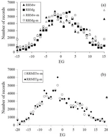
farm-year groups. In the third and fourth RRMs, the EGs were based, respectively, on the average W450 (RRMw-m) and the average G450 (RRMg-m) of farm-year-season-management groups. As farm-year-season-management has an implicit sex factor, the records were separated according to sex, and af-ter definition of the environmental groups as standardized W450 averages, the data of the different sex groups were merged by EGs. EG values below -15 were considered in EG = -15 (bottom limit) and those above +15, in EG = +15 (upper limit) (as shown in Figure 1a). The fifth random re-gression model (RRMITw-m) used an iterative algorithm to define the EGs. In the first iteration, the data were ana-lyzed using RRMw-m and its fixed effect (CG) solutions were used to position records on the respective EG for the subsequent analysis. Since this first iteration resulted in a wide data distribution along the environmental gradient the EG limits were changed to -20 (bottom limit) and +20 (up-per limit) from the second to the final iteration (Figure 1b). The process was stopped when the correlation between the EG positions in the previous and present analyses was > 0.999. This convergence was reached after three itera-tions, in a manner similar to the simulated data used by Caluset al.(2004). This process tries to avoid bias resulting from the non-random use of sires or a low number of ani-mals in some herds. The last random regression model (RRMITg-m) used G450-based EGs in the first iteration and repeated the RRMITw-m iterative process.

The EGs were defined using the complete dataset, but additional restrictions were added for parameter estima-tion. In this case, sires were excluded if (1) they had < 100 progeny weights and (2) the progeny weight distribution along the environmental gradient was < 20 EG units (before the first iteration in RRMITw-m and RRMITg-m). After application of these two criteria, CGs with less than five re-cords were removed. These restrictions affected data differ-ently in the different models and resulted in different numbers of sires and records for the analyses. The UM esti-mates were based on RRMw data.

(Co)variances of random regression coefficients were estimated by REML using version 3.0bof the DFREML package (Meyer, 1988). The DXMRR subroutine in the program allowed estimation of the heterogeneous residual variance in five classes. Estimates were obtained by using Powell, Simplex and AI-REML algorithms, thereby avoid-ing problems with “derivative-free” possible local max es-timates. The general model can be represented as follows:

yij Fij m m EGij EG

m k

im m ij ij

m k a a = + + + = -=

-å

å

0 1

0 1

whereyijis thejthprogeny’s W450 or G450 from theith

ani-mal andEGijis the environmental group of thejthprogeny

ofithsire (from -15 to +15 in non-iterative models and -20 to +20 in iterative models),fm(EGij)is themthLegendre

poly-nomial on environmental group,Fijis the CG fixed effect,

bmis the fixed regression coefficient to model the

popula-tion mean (defined only in non-iterative models),amis the

random regression coefficient for a direct genetic effect,ka

denotes the corresponding orders of fit (one in UM and two for RRMw, RRMg, RRMw-m, RRMg-m, RRMITw-m and RRMITg-m) andeijis the error effect associated with the

pre-defined classespthat have homogeneous variances. In matrix notation:

y=Xb+Zs+e

where E y s X = é ë ê ê ê ù û ú ú ú = é ë ê ê ê ù û ú ú ú e b 0 0

and V s K A R s e é ë ê ù û

ú =é Ä

ë ê ù û ú 0 0

with y being the vector of observations,bthe vector of fixed effect attributable to contemporary groups (includ-ingFijandbm),sthe vector of sire random coefficients,X,Z

the corresponding incidence matrices, andethe vector of residuals.Ksis the matrix of coefficients of the covariance

function for sire effect,Ais the additive numerator relation-ship matrix andRis the diagonal matrix of residual vari-ances estimated at five levels. The levels of s$e p

2 , with p = 1,2,3,4,5 were grouped in EGs from -15 to -9, -8 to -3, -2 to +2, +3 to +8, and +9 to +15, respectively, for non-iterative models, and -20 to -12, -11 to -4, -3 to +3, +4 to

+11, and +12 to +20, respectively, for iterative models. These groups were accommodated by identities matrices of appropriate order for each level.

Direct additive variance estimates in the random re-gression sire model were obtained by multiplying sire vari-ance estimates by four (s$A s$s

2 2

4

= ). Residual variance esti-mates were obtained as the difference between phenotypic variance (s$P s$s s$e p

2 ₌ 2₊ 2

) and additive variance estimates (s$_E2 ₌s$_P2 _-s$_A2)

. Expected breeding values (EBVs) were the double of expected progeny differences (EPDs), the lat-ter being obtained from the sire model directly by the equa-tion:

EPD_{i EG} im m EG

m ka =

=

-å

0 1

Results

The distributions of animal weights along the envi-ronmental gradient in RRMg and RRMg-m (based on G450) were skewed slightly to the right (skewness of 0.15 and 0.16, respectively). Data distribution in RRMw and RRMw-m was less symmetric, with skewness of 0.67 and 0.70, resulting in the accumulation of records in EG = +15 (Figure 1a). When EGs were defined based on farm-year groups the records were concentrated in the central region of environmental gradient and led to a larger number of sires being excluded from the analysis compared to the farm-year-season-management groups (192 and 177 sires with 85,259 and 79,250 total records in RRMw and RRMg, and 220 and 242 sires with 89,784 and 90,735 total records in RRMw-m and RRMg-m and their iterative models, re-spectively).

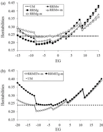
Table 1 shows the parameter estimates of the model (with approximate standard errors for the Legendre polyno-mial coefficients and residual variances) in different analy-ses. In UM, there were only single estimates for residual variance and genetic variance. Hence, in Figure 2 and in the Supplementary Material, the variances are shown as lines to allow visual comparisons with RRMs (the lines are par-allel to the environmental gradient axis).

unfa-vorable environments, but this situation was inverted in the favorable extreme, where the estimate was highest. The UM heritability estimate (h2 = 0.24) was lower than the RRM estimates along most of the environmental gradient, with larger differences in the favorable extreme. Different changes occurred when iterative models were applied to W450- and G450-based environmental variables. RRMITw-m and RRMw-m had a very similar shape, whereas RRMITg-m and RRMg-m showed important dif-ferences in extreme environments, with much higher heritabilities after iterations. Indeed, RRMITg-m had the highest heritabilities of all of the models.

Partitioning the estimates of residual variance into five levels based on a continuous additive genetic variance created abrupt leaps in the curves of residual and pheno-typic variance estimates and indicated intense heterosce-dasticity along EG levels. Phenotypic variance estimates

(s$P) 2

tended to increase along the environmental gradient as a whole and showed stable values within residual estimate classes. The additive genetic variance estimates(s$A)

2 were greater at the extremes of the environmental gradient in all models. Residual variance estimates (s$E)

2

increased slightly along the environmental gradient but were variable within classes (they increased when p = 1, were stable when p = 2, and decreased when p = 3 to 5). The variance compo-nents estimates are shown in the Supplementary Material (Figures S1-S3).

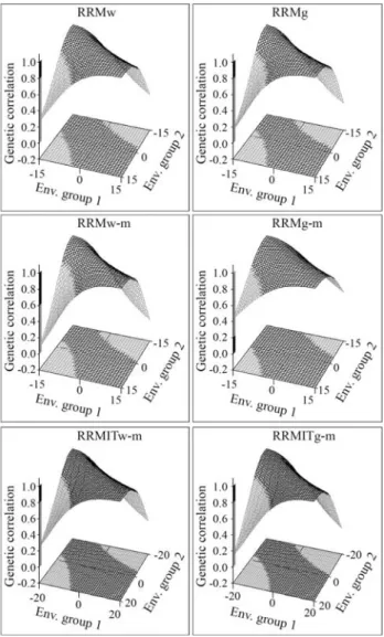
RRMs estimated the covariance functions and dis-played the genetic correlation estimates (rg) between

envi-ronments as surface three-dimensional plots (Figure 3). The rgwere plotted on the z axis based on EG values for the

x and y axes. This resulted in figures with “saddle” shapes

in which rgwas minimal between opposite extremes

(rang-ing from 0.08 in RRMw to 0.47 in RRMITw-m) and close or equal to one among similar environments in favorable or unfavorable regions. All of the models revealed a marked

Table 1- Random regression sire variance estimates of the Legendre polynomial intercept (I, k = 1) and slope (S, k = 2), covariance (IxS) and residual variance estimates for different classes (p from 1 to 5) in different models (UM, RRMw, RRMg, RRMw-m, RRMw-g, RRMITw-m, RRMITg-m). The approximate standard errors are shown below each parameter.

Intercept (I) (k = 1)

Slope (S) (k = 2)

I x S s$e p=1 2 _s$

e p=2

2 _s$

e p=3 2 _s$

e p=4 2 _s$

e p=5 2

UM 80.6 629.2

5.6 6.9

RRMw 66.9 19.3 14.4 478.1 562.4 590.3 664.0 738.84

6.2 4.7 3.8 11.8 10.1 15.5 26.9 40.6

RRMg 72.0 18.3 16.6 530.1 575.5 636.6 628.4 762.8

6.8 5.3 4.1 12.6 9.8 13.8 22.3 43.8

RRMw-m 71.9 14.5 12.8 479.4 553.8 614.9 657.1 763.7

6.1 3.9 3.5 10.3 9.5 14.4 24.0 43.1

RRMg-m 81.9 11.2 9.6 523.2 592.8 621.9 630.3 750.5

6.6 3.3 3.0 9.5 9.2 11.8 16.4 33.4

RRMITw-m 77.2 16.6 16.6 476.1 564.6 617.3 681.5 854.0

6.9 4.4 4.6 9.4 9.2 16.1 29.4 55.6

RRMITg-m 81.3 12.5 20.8 483.6 575.6 604.2 671.8 839.0

6.5 4.1 4.7 9.4 8.8 13.4 21.4 42.7

GEI between opposite extreme environments. The genetic correlation value of 0.8, which is indicative of a significant GEI (Robertson, 1959), separated the black part of the

sur-face with less important GEI (rg> 0.8) from the grey part

with important GEI (rg < 0.8). RRMg, RRMw-m and

RRMITg-m yielded lower correlations between opposite extremes and had larger grey areas on the surface. RRMg-m had a higher rgand smaller grey areas. RRMw

and RRMITw-m were intermediate in their ability to iden-tify GEI.

Adaptive reaction norms (ARN) were defined using predicted genetic values expressed as expected progeny differences (EPDs) along the environmental gradient. A sample of ARNs is shown in Figure S4. The ARN slopes in-dicate the angular coefficient of the sires’ ordinary polyno-mials. These values were used in regression analyses to identify biases in the current selection programs. Regres-sion analyses of the UM EPDs (constant and independent of environmental gradient) on RRM EPDs in EGs -15, zero and +15 in non-iterative models, and EGs -20, zero and +20 in iterative models, as well as on slopes, yielded significant results (p < 0.0001). The correlation between UM EPDs and favorable environment RRM EPDs (EG = +15) was positive and even greater (Table 2). The correlations be-tween UM EPDs and ARN slopes ranged from 0.64 to 0.72. The variance of the ARN slope is directly related to the importance of GEI and reflects the environmental sensi-tivity (Falconer, 1990), referred to as plasticity (in relation to larger absolute slopes) or robustness (in relation to smaller absolute slopes). Regression analyses for ARN slopes from different RRMs were consistent (p < 0.0001) and had coefficients of determination between 0.70 (RRMg X RRMg-w) and 0.98 (RRMw-m X RRMITw-m). Figure S5 shows the regressions and their equations and coeffi-cients of determination.

Discussion

The results described here show that different models generate consistent parameter estimates. The initial aim of using different environmental descriptors was to maximize the identification of GEI based on the concept that similari-ties between independent (EGs of W450 averages) and

de-Table 2- Correlation coefficients for the linear regression between expected progeny differences (EPDs) from UM and other models at specific points in the environmental gradient (EG = -15, 0 and +15 for RRMw, RRMg, RRMw-m and RRMg-m, and EG = -20, 0 and +20 for RRMITw-m and RRMITg-m). Only sires with progeny weights that were used in the analyses were considered (p < 0.0001 for all regressions).

RRMw RRMg

EG(-15) EG(0) EG(+15) Slope EG(-15) EG(0) EG(+15) Slope

UM 0.77 0.99 0.96 0.76 0.66 0.97 0.92 0.64

RRMw-m RRMg-m

EG(-15) EG(0) EG(+15) Slope EG(-15) EG(0) EG(+15) Slope

UM 0.85 0.99 0.97 0.75 0.88 0.97 0.96 0.72

RRMITw-m RRMITg-m

EG(-15) EG(0) EG(+15) Slope EG(-15) EG(0) EG(+15) Slope

UM 0.86 1.00 0.97 0.76 0.78 0.97 0.94 0.69

pendent (variance components and EPDs for W450) regression variables would lead to biases and lower signifi-cance of GEI. This occurred when comparing the RRMITw-m and RRMITg-m genetic correlation surfaces, but was not directly observed among non-iterative models or when heritabilities were considered. The low genetic correlation among extreme environments suggested that different groups of genes were being expressed. In agree-ment with Falconer (1960), we suggest that growth in low or high nutritional environments results in the differential expression of genes associated with growth and feed intake and efficiency. This affirmation, together with the results of the UM EPD regression analysis, indicates that current se-lection programs may be selecting for greater growth and feed intake, regardless of the feed efficiency. Environmen-tal gradients, when defined by the CG averages, can gener-ate connections among dependent and independent model variables that only can be explained by Wright’s path anal-ysis. This methodology is recommended by Lynch and Walsh (1997) for studies with related components in which correlations among indicators of latent (non-measurable) variables and the path coefficients are defined using struc-tural equation models with simultaneous dependencies. Future work could examine the correlations and path coef-ficients for latent variables (gene group effects related to different trait components) in different environments. Such an analysis could help to explain differences in the impor-tance of GEI and heritabilities in various RRMs since envi-ronmental descriptors generally correlate with the causal components of weight trait.

The importance of GEI in weight trait and the useful-ness of the reaction norm concept as an effective model in this case need to be emphasized. Even so, choosing the best environment descriptor apparently depends on the desired breeding goal. Complex relationships among trait compo-nents are tied to the breeding goal and the model of choice can be indicated by larger genetic gains by generation for the chosen environments. With reaction norms, robustness and plasticity can be added as additional breeding goals to generate options for generalist or specialist sires.

In conclusion, we have demonstrated an important genotype-by-environment interaction in the 450-day weight trait of Nelore cattle analyzed by random regression reaction norm models using environmental variables de-fined by group averages. Genetic correlations were low be-tween opposite extreme environments. These data indicate a significant re-ranking of sires in different environments and show the need to consider GEI effects, not only in large scale (across countries), but also within a national analysis. The UM EPDs showed a lower correlation with EPDs in unfavorable compared to intermediate and favorable envi-ronments, indicating that selection based on the predictions of UM genetic values is biased towards favorable environ-ments.

Although the parameter estimates for the different models showed a joint variable tendency along the environ-mental gradient, changes in the environment descriptor in-terfered with these values. Iterative models amplified the distribution of data along the environmental gradient and yielded higher heritabilities. The use of G450-based envi-ronment descriptors altered the estimates of variance. This finding suggested the presence of intrinsic correlations with other genetic variables linked to physiological and morphological characters that make up the W450 trait. Such an association would explain the increase in herita-bility at unfavorable environmental extremes.

Acknowledgments

We thank the National Association of Cattle Breeders and Researchers (ANCP) for providing access to the data-base, and to Drs. Alessandro Antonangelo, Pedro Luiz Bicudo and Klaus Hartfelder for suggestions about the manuscript. This study was supported by CAPES.

References

Albuquerque LG and Meyer K (2001) Estimates of covariance functions for growth from birth to 630 days of age in Nelore Cattle. J Anim Sci 79:2776-2789.

Bolton RC, Frahm RR, Castree JW and Coleman SW (1987) Ge-notype X environment interactions involving proportion of Brahman breeding and season of birth. I. Calf growth to weaning. J Anim Sci 65:42-47.

Calus MPL, Bijma P and Veerkamp RF (2004) Effects of data structure on the estimation of covariance functions to de-scribe genotype by environment interactions in a reaction norm model. Genet Sel Evol 36:489-507.

De Jong G and Bijma P (2002) Selection and phenotypic plasticity in evolutionary biology and animal breeding. Livest Prod Sci 78:195-214.

De Mattos D, Bertrand JK and Misztal I (2000) Investigation of genotype x environment interactions for weaning weight for Herefords in three countries. J Anim Sci 78:2121-2126. El Hani CN (2007) Between the cross and the sword: The crisis of

the gene concept. Genet Mol Biol 30:297-307.

Falconer DS (1960) Selection of mice for growth on high and low planes of nutrition. Genet Res 1:91-113.

Falconer DS (1990) Selection in different environments: Effects on environmental sensitivity (reaction norm) and on mean performance. Genet Res 56:57-70.

Fikse WF, Rekaya R and Weigel KA (2003) Assessment of envi-ronmental descriptors for studying genotype by environ-ment interaction. Livest Prod Sci 82:223-231.

Johnston DJ, Reverter A, Burrow HM, Oddy VH and Robinson DL (2003) Genetic and phenotypic characterization of ani-mal, carcass, and meat quality traits from temperate and tropically adapted beef breeds. 1. Animal measures.Austr J Agric Res 54:107-118.

Kirkpatrick M and Heckman N (1989) A quantitative genetic model for growth, shape and other infinite-dimensional characters. J Math Biol 27:429-450.

cattle studied using reaction norms. Acta Agric Scand A Anim Sci 52:11-24.

Kolmodin R, Strandberg E, Danell B and Jordani H (2004) Reac-tion norms for protein yield and days open in Swedish Red and White dairy cattle in relation to various environmental variables. Acta Agric Scand A Anim Sci 54:139-151. Lewontin RC (1998) The Triple Helix: Gene, Organism and

Envi-ronment. Harvard University Press, Cambridge, 192 pp. Lynch M and Walsh B (1997) Genetics and Analysis of

Quantita-tive Traits. Sinauer Associates, Sunderland, 980 pp. Meyer K (1988) DFREML - A set of programs to estimate

vari-ance components under an individual animal model. J Dairy Sci 71:33-34.

Meyer K (1998) Estimating covariance functions for longitudinal data using a random regression model. Genet Sel Evol 30:221-240.

Mulder HA and Bijma P (2005) Effects of genotype X environ-ment interaction on genetic gain in breeding programs. J Anim Sci 83:49-61.

Nobre PRC, Rosa NA and Euclides Filho K (1988) Interação reprodutor X estação de nascimento e reprodutor x fazenda sobre o crescimento de bezerros Nelore. Rev Bras Zootec 17:120-131 (Abstract in English).

Robertson A (1959) The sampling variance of the genetic correla-tion coefficient. Biometrics 15:469-485.

Sarkar S (1999) From the Reaktionsnorm to the adaptive norm: The norm of reaction, 1909-1960. Biol Phil 14:235-252. Schlichting CD and Pigliucci M (1998) Phenotypic Evolution: A

Reaction Norm Perspective. Sinauer Associates, Sunder-land, 387 pp.

Schmalhausen II (1949) Factors of Evolution: The Theory of Sta-bilizing Selection. The Blakiston Company, Philadelphia, 327 pp.

Veerkamp RF and Thompson RA (1999) A covariance function for feed intake, live weight and milk yield estimated using random regression model. J Dairy Sci 82:1565-1573.

Supplementary Material

The following online material is available for this ar-ticle:

Figure S1 - Phenotypic variance estimates (in kg.kg) along environmental group (EG) in UM, RRMw, RRMg, RRMw-m and RRMw-g (a) and UM, RRMITw-m and RRMITg-m (b).

Figure S2 - Genetic additive variance estimates (in kg.kg) along environmental group (EG) in UM, RRMw, RRMg, RRMw-m and RRMw-g (a) and UM, RRMITw-m and RRMITg-m (b).

Figure S3 - Residual variance estimates (in kg.kg) along environmental group (EG) in UM, RRMw, RRMg, RRMw-m and RRMw-g (a) and UM, RRMITw-m and RRMITg-m (b).

Figure S4 - Adaptive reaction norms (ARNs) of “top 10 UM EPDs” sires, expressed in EPDs (in kg) plotted along the environmental gradient (EG) for different models (RRMw, RRMg, RRMw-m, RRMg-m, RRMITw-m and RRMITg-m).

Figure S5 - Regressions between 450-day weight ARN slopes estimated by different models (RRMw x RRMg, RRMw-m x RRMw, RRMg-w, RRMg x RRMg-m, RRMw-m x RRMg-m, RRMITw-m x RRMw-m and RRMITg-m x RRMITw-m), with their respective regres-sion equations and regresregres-sion coefficients (R2) (p < 0.0001 for all regressions).

This material is available as part of the online article from http://www.scielo.br/gmb.

Associate Editor: Pedro Franklin Barbosa

group (EG) in UM, RRMw, RRMg, RRMw-m and RRMw-g (a) and UM, RRMITw-m and RRMITg-m (b).