Equivalent Models and Exact Linearization by the Optimal Control of Monod Kinetics Models

(1)

Equivalent Models and Exact Linearization by the

Optimal Control of Monod Kinetics Models

Yuri Pavlov, Krassimira Ljakova

Centre of Biomedical Engineering, Bulgarian Academy of Sciences 105, Acad. G. Bonchev Str., Sofia 1113, Bulgaria

E-mail: yupavlov@clbme.bas.bg

krasil@clbme.bas.bg

Abstract: The well-known global biotechnological models are linear and non-stationary. In addition the process variables are difficult to measure, the model parameters are time varying, the measurement noise and measurement delay increase the control problems, etc. One possible way to solve some of these problems is to determine the most simple and easy for use equivalent models. The differential geometric approach [DGA] and especially the exact linearization permit an easy application of the optimal control. The approach and its application in the control of the biotechnological process are discussed in the paper. The optimization technique is used for fed-batch and continuos biotechnological processes when the specific growth rate is described by the Monod kinetics.

Keywords: Biotechnological process, Exact linearization, Pontryagin maximum principle, Brunovsky normal form.

Introduction

The control systems are already implemented in modern bioreactors. From biotechnological

point of view the straightforward way of improving the economics is to invest in process

optimization and control.

The fermentation processes are complex ones and the well-known biotechnological models

are non-linear and non-stationary. They are attractive and difficult objects for control,

particularly when for the control variable is accepted the dilution rate. Many mathematical

models have been proposed but just few have been used successfully because of the

peculiarities of the bioprocesses. The conventional linear systems of control and the

conventional control methods are used extensively but not in all cases with success [10, 11,

13]. In addition the process variables are difficult to measure and the model parameters are

time varying. The measurement noise and the parameters identification delay increase the

(2)

impossible without automatic measurement and control. Any real control scheme must take

these factors into consideration. Control design methodologies, which take into accounts the

robustness properties of the control design, appear highly attractive for control of

biotechnological process. Consequently the elaboration and the design of new control systems

in the field of biotechnology is an open automation problem.

The mentioned above determines the biotechnological systems and controls like a specific

domain of investigations with specific problems and tasks. Very promising in this field is the

exact linearization approach that based on the DGA and the GS algorithm [4]. Such approach

permits successful utilization of the maximum principle for the determination of the optimal

control [1, 2, 3, 4].

Problem statement

The aim of the paper is to demonstrate the possibilities of an integral approach for control

determination that include the DGA exact linearization and the Pontryagin maximum

principle.

Mathematical models – continuous process

The continuous biotechnological process is a continuously operated bioreactor with one

substrate in the feed. The bacterial biomass consumes the substrate to produce more biomass,

and the biomass is harvested as the desired end product. The state variables are the biomass

(bacterial cell mass) and the substrate concentrations in the bioreactor as a function of the

time. The modelling approach in [11, 12, 13, 14] is analysed as a feasible base for control

design. In this model Stephanopoulos and San introduced a state variable (colour noise) to aid

the convergence of the specific growth rate in the model. After linearization the linear model

was not controllable, that is why Wang and all proposed a modification of the dynamic model

for the specific growth rate in which are included the maximum growth rate, the

Mihaelis-Menten constant and a white noise process. The so defined model is:

(1)

Where:

-X is the biomass concentration in the bioreactor,

ν

S K

S µ m

D S S X y S

DX X X

+ − + =

− + −

=

− =

) (

1

s m

0

µ µ

(3)

-S is the substrate concentration, -µ is the specific growth rate,

-Ks is a saturation coefficient (the Mihaelis-Menten constant),

-ν is a white noise process,

-S0 is the substrate concentration in the feed,

-m is a constant determining the dynamic of the growth rate, -D is the dilution rate,

-µm (T, pH) is the maximum growth rate (as a function of the temperature and the acidity of

the bioreactor medium pH),

-y biomass yield with respect to substrate.

This model with the third equation is an extension of the well-known Mono model.

The system set point is given by the next expression:

(2)

where

-X10 is the biomass concentration in the set point,

- Se≡ (x20) is the substrate concentration in the set point,

-µ30 is the specific growth rate in the set point,

-De is the dilution rate in the set point.

The system operation conditions were fixed by the following set of values: µm=0.5 h-1,

Ks=0.05 g.l-1, m=3, Se=0.2625 g.l-1, S0=9 g.l-1, y=0.5 g.g-1, De=0.42 h-1.

The noise was taken 0%. The performance of the system without control is shown in Fig. 1.

Fig.1 Model (1) - without control Fig.2 Models (1) and (8) – without control e

e e e

S S y X

S K

S µ D

− =

+ =

=

0 10

s m 30 30

µ

0 1 2 3 4 5 6 7 0

1 2 3 4 5 6 7

time [h]

X [g/l]

S [g/l]

µ

0 1 2 3 4 5 6 7

-2 -1 0 1 2 3 4 5 6 7

time [h] X [g/l]

S [g/l]

µ

Y3

(4)

A complication is that the diffeomorphism defining the equivalent nonlinear transformation

from the nonlinear system (1) to the Brunovsky normal linear form is non-regular in the

equilibrium point [2, 8]. In the limits the two models (the nonlinear model and the Brunovsky

model) converge to the equilibrium points. From computing point of view in the limits arise

rounding problems. We escape in parts this problem, taking in account that some evaluations

of the state vector coordinates around the set point are influenced faintly. This fact forces a

new model determination, in which the third differential equation has a polynomial form (3)

where c=0.42, m1=0.0286, m2=0.713 [7, 11, 13].

The next two vectors determine the affine space of the new nonlinear system. The vectors f0

and f1 determine the appropriate linear space:

(3)

Where c, m1 and m3 are constants that determined the evaluation of the model around the set

point (dz/dt=f0+f1.U, where U =D is the control input and z=(X,S,µ).

Mathematical models – fed batch process

The well-known non-linear model [5, 6, 11, 13] describes the fed batch process:

(1*)

Where F is the substrate-floating rate and Vo is the volume of the bioreactor. In the paper the DGA is used for the model (3) and model (1*). The DGA demonstrated in the paper is

completely applicable for the model (1) too. The inputs of these models are the dilution rate

and the substrate-floating rate.

⎟ ⎟ ⎟

⎠ ⎞

⎜ ⎜ ⎜

⎝ ⎛

− − =

⎟ ⎟ ⎟ ⎟ ⎟ ⎟ ⎟

⎠ ⎞

⎜ ⎜ ⎜ ⎜ ⎜ ⎜ ⎜

⎝ ⎛

− −

− =

0 1

3 1

0 S S

X

) m X m m(c

X y

X

f f

µ µ

µ

F Vo

S s K

S m

S S Vo

F X k S

X Vo

F X X

m

=

− + =

− +

− =

. .

0 .

.

) (

µ

(5)

⎟

⎠

⎞

⎜

⎝

⎛ −

=

⎟

⎠

⎞

⎜

⎝

⎛

−

+

=

0

0 m

1

3 2 2

2 2 3 2

3

1 3

0

x

)

x

z

K

z

m( µ

x

y

x

S

f

Brunovsky normal form and exact linearization - continuos process

There are difficulties with the linear systems. In some case of the classical linearization the

correspondence between the biotechnological process and it linear model is lost. The reason is

in the strong non-linearity of the models (1, 1*). In addition the optimization methods like

Pontryagin maximum principle are difficult for direct use [3]. Here is proposed a DGA for

exact linearization that is a consequence from a non-linear diffeomorphic transformation.

Consider the continuous process described by the non-linear model (1). The system operation

conditions are fixed by the following set of values: µm=0.5 h-1, Ks=0.05 g.l-1, m=3, Se=0.2625

g.l-1, S0=9 g.l-1, y=0.5 g.g-1, De=0.42 h-1, we determined the basis of the appropriate affine

space:

The control input is the dilution rate D. Taking in account the common integral of the field f1

the model (1) is transformed with the next diffeomorphic transformation:

where z=(X,S,µ) is the state vector of model (1). The affine model has the next basis:

(4)

In what follows in this paragraph the vector z=(X, S, µ) is the state vector of the model (1) and the vector x=(x1, x2, x3) is the state vector of the model (4). The t-differential forms corresponding to the model (4) defined by f0 and f1 are the next [2]:

⎟ ⎟ ⎟

⎠ ⎞

⎜ ⎜ ⎜

⎝ ⎛

− − =

⎟ ⎟ ⎟ ⎟ ⎟ ⎟ ⎟

⎠ ⎞

⎜ ⎜ ⎜ ⎜ ⎜ ⎜ ⎜

⎝ ⎛

− + − =

0 m

1

0 1

3

0 S S

X

) x S K

S m(

X y

X

S

f f

µ µ

µ

= − = =

3

0 2

1

), tion Transforma (

, x

S S

X x

(6)

V

y

=

3 3 2 2 1 . . . (5)

According the denotations and the notions in [2] the dual co-distribution (dual vector space)

range is:

(6)

The set K0={w1, w2}, K1={w1} and K2=∅:

(7)

Considering the dual range (6) the equivalent system has the next Brunovsky normal form:

(8)

All regular conditions are fulfilled excepting in the set point (equilibrium). The diffeomorphic

transformation from system (4) to system (8) is a consequence from the dual range (6) [2, 8]:

Therefor the nonlinear transformation has the form [2]:

(

K

S

)

x

y

x

t

x

S

x

m

x

y

x

y

x

y

x

y

x

y

x

y

t

)

x

y

x

y

w

S

d

)

1 )(

(

)

2

3 (

d

)d

1 (

)d

2

1 (

d

1 (

d

2 2 2 3 1 0 2 1 0 2 m 3 2 2 2 2 2 2 3 2 2 3 2 2 2 2 2 3 2 2 2 2 3 1 1

⎭

⎬

⎫

⎩

⎨

⎧

+

−

+

−

=

+

=

+

−

=

µ

(

)

)(

1 )

(

)

2

3 (

)

1 (

2 2 2 3 1 0 2 1 0 2 m 3 2 2 2 2 2 2 3 3 2 2 2 3 2 2 1

x

y

x

S

K

x

S

x

µ

m

x

y

x

y

x

y

x

y

x

y

x

y

S

+

−

+

=

+

=

0 d

d

)

s

(

s

µ

2

1

2 d

,

)d

)

s

(

µ

(

d

2 ,

)d

1 (

d

1

3 2 1 2 1 0 2 2 m 3 1 2 0 2 0 1 m 3 2 2 3 2 3 2

≠

∧

+

=

∧

−

+

−

=

+

−

=

x

t

x

S

K

x

K

m

w

t

x

S

K

x

S

x

m

x

w

t

x

y

x

w

i i 1

i d 0mod K K

K ⇔ = ∈

∈ ₊ w , w

w

2 1

0

K

(7)

m

x

m

x

m

c

x

y

x

mm

x

y

x

y

x

y

x

y

x

m

x

m

c

m

x

y

x

y

x

U

x

y

x

mm

V

)

(

)

1 (

)

2

3 (

2 )

1 (

)

2

1 )(

(

)

6

1 (

)

)(

1 (

3 3 1 1 2 2 2 3 3 2 2 2 2 2 3 2 2 2 3 2 3 3 1 1 2 2 2 2 2 3 1 1 3 2 2 2 1

−

⎭

⎬

⎫

⎩

⎨

⎧

₊

₋

₊

+

⎭

⎬

⎫

⎩

⎨

⎧

+

−

+

−

+

−

=

The comparison of the model (1) and the model (8) evaluations is shown in Fig. 2. There are

computer-rounding problems with model (8) because of the fact that the set point is

non-regular. A new model (3) of polynomial form has been proposed (c=0.42, m1=0.0286,

m2=0.713). The affine representation of this model is [7, 8]:

It overcomes in parts the computer-rounding problems. The equivalent non-linear

transformation from the model (3) to the Brunovsky normal form (8) is:

(9)

The control V of the Brunovsky model is linked with the control U=D of the model (1, 3) with the formulae:

(10)

The control input U of the model (1) is in fact the dilution rate D. Evaluations of the model (8) are calculated with the diffeomorphism described by (9):

Model (1) == (Transformation K)===> Model (4)==(Transformation 9)===> Model (8)

(8)

3 2 2 1 3 2 1 2 1 1 3 3 2 2 1

2 T

T

H

C

t

C

t

C

T

C

t

C

T

C

T

V

y

+

−

=

+

−

=

+

=

Direct application of the Brunovsky model is the analytical determination of the optimal

control in order to reach the set point for minimal time. The Hamilton function has the form:

We suppose t∈[t0, t1] and like optimization criterion is chosen min F(x(t1))=[x1(t1)-x10]2,

where x10=4.37, where x1 is the first variable in the model (3). The formulae x1(y1, y2, y3) has

the next huge form:

1 3 2 1 1 2 1 2 1 1 3 1 2 2 1 1 2 2 1 1 2 2 3 1 1 ) 1 ( ) 1 ( 1 ) 2 3 ( ) 1 ( 1 m m y y y y m c y y y m y y y y y y y y y y m x + + − + ⎥ ⎥ ⎥ ⎥ ⎦ ⎤ ⎢ ⎢ ⎢ ⎢ ⎣ ⎡ + + + − =

Finally the optimal control has the next functional form (11) (max (H)):

(11)

The function g(.) in formulae (11) connect the optimal control V with the optimal control U in formulae (10). Taking in account the conditions for optimal control we found that the

constants C1 and C2 have the forms:

The constant C3 presents the similar huge formulae like C1. The constants A and B were

derived from C1, C2 andC3.

)

y

1 y

(

1 mm

)

37 .

4 x

(

2 B

2 1 1 1 1

+

−

=

⎪ ⎪ ⎭ ⎪⎪ ⎬ ⎫ ⎪ ⎪ ⎩ ⎪⎪ ⎨ ⎧ + + + + + + + + − + − − = ) 1 ( ) 2 1 ( ) 1 ( ) 2 1 ( ) 1 ( ) 2 1 ( 2 ) 1 ( 2 ) 37 4 ( 2 2 1 1 1 1 2 3 2 2 1 1 1 3 3 2 1 1 2 1 2 2 2 1 1 2 2 1 1 1 y y y m y y y m y y y y y y y y y y y y y y y y y mm . x C 1 1 2 1 1 1 3 1 2 2 1 1 1 2 1 1 2 ) 1 ( 1 ) 37 4 ( 2 ) 1 ( ) 2 1 ( 2 ) 37 4 ( 2 t C y y y m m . x y y y y y y mm . x C + + − + + + − − = ) 1 ( 1 ) 37 4 ( 2 ) 1 ( ) 2 1 ( 2 ) 37 4 ( 2 2 1 1 1 3 1 2 2 1 1 1 2 1 1 y y y m m . x y y y y y y mm . x A + − + + + − − =

)

,

)

1 (

B

)

(

A

)

(

2 (sign

V

1 1 1 1 12 1 2 3

2 1

1

_y

_U

_x

(9)

0 1 2 3 4 5 6 7 -1

0 1 2 3 4 5 6 7 8 9

tim e [h] X [g/l]

S [g/l]

B runovsky m odel (8) - Y 2

O ptim al control - V

0 1 2 3 4 5 6 7

- 2 - 1 0 1 2 3 4 5 6 7 8

tim e [h ] Y 2

Y 3

Y 1

Fig.3 Models (3) and (8) – optimal control Fig.4 Brunovsky model (8)

The constants C1, C2 and C3 were calculated at the moment t1. If the optimal control is

calculated by iterations from [ti, ti+1] and these intervals are relatively small, we find the

formulae for V. The optimal evaluations of the models (3 and 8) are shown in Fig. 3. The deviations of the Brunovsky model with this control are shown on Fig. 4.

Brunovsky normal form and exact linearization - fed-batch process

The well-known non-linear model [1, 2] describes the fed batch process:

(1*)

Here X is the biomass concentration, S is the substrate concentration, µ is the specific growth rate, Vo is the volume of the bioreactor. The maximum growth rate is noted as µm and KS is a

saturation coefficient and k=1/y where y=0.5 [11, 12, 13, 14].

The growth dynamics are modelled by the third equation according Stephanopulos. The

control input is F. The basis of the appropriate affine space is [2]: F

Vo

S s K

S m

S S Vo

F X k S

X Vo

F X X

m

=

− + =

− +

− =

. .

0 .

.

) (

µ

(10)

dt

du

w

dt

S

s

K

S

m

du

w

dt

u

y

u

du

w

m

µ

−

=

−

+

−

=

+

−

=

4 3 3 2 2 2 2 2 1

,

)

(

,

)

1 (

⎟

⎠

⎞

⎜

⎝

⎛

−

+

−

=

0 )

(

0

µ

S

s

K

S

m

X

k

X

m

f

⎟ ⎟ ⎟ ⎟ ⎟ ⎟ ⎠ ⎞ ⎜ ⎜ ⎜ ⎜ ⎜ ⎜ ⎝ ⎛ − − = 1 0 ) (S - 0 1 Vo S Vo X f

⎟

⎠

⎞

⎜

⎝

⎛

−

+

=

µ

)

(

2 2 2 0

S

s

K

S

m

u

k

u

X

m

f

⎟⎟

⎟

⎠

⎞

⎜⎜

⎜

⎝

⎛ −

=

0

1

Vo

X

f

(12)

The next step is a simplification of the basis of the affine model space. We transform the state

vector x=(X, S, µ, Vo) of the model (1*) with the use of the common integrals of the field f1.

The transformation is:

(13)

The new affine model has the next basis:

(14)

The new affine model has the form du/dt=f0+f1F, were u=(u1, u2, u3, u4), x=(x1, x2, x3, x4)= =(X, S, µ, Vo). The t-differential forms corresponding to the model (14) affine space defined by f0 and f1 are the next:

(15)

After the denotations and notions in [2] the dual co-distribution (dual vector space) range is:

(16)

Where the set K0={w1, w2, w3}, K1={w1, w3} and K2=∅. Here is used the theorem 1.23 of [2]:

⎟

⎠

⎞

⎜

⎝

⎛

+

−

=

⎟⎟

⎟

⎠

⎞

⎜⎜

⎜

⎝

⎛

)

(

log

)

(

log

)

,

(

1 2 3 4 0

4 3 2 1

Vo

X

S

X

x

u

µ

Φ

2 1

0

K

(11)

i i

i dw w

w ∈ K + 1 ⇔ = 0 mod K , ∈ K

4 1 2 3 3 2 2 4 1 3 4 1 3 2 4 1 1

)

(

x

s

K

x

m

x

Y

x

Y

x

Y

m

−

=

+

−

+

=

)

(

µ

4 4 2 2 2 3 3 2 2 2 2 2 2 3 2 2 2 2 2 1 ) 1 )( ) ( ( ) 2 3 ( ) ( u Y u y u x S s K S m u y u y u Y ku u Y u Y m = + − + + + + = + = =

µ

(17)

From the dual range (1) the equivalent diffeomorph model has the form:

(18)

All regular conditions are fulfilled excepting in the points where the denominator of the

differential form dw2 is zero. The diffeomorphism from the model (14) to the model (18) is a

consequence from the dual range [2, 5, 6]:

(19)

From the formulae (19) follows the next diffeomorphism:

(20)

If we start from different form of the model (1*) with the same mathematical technique we

determine the next diffeomorphism:

(21) dt u y u u x s K x m u y u y u u dY dY du u y u du u y u dY dt u y u u dy w m ) 1 )( ( ) 2 3 ( ) 1 ( ) 2 1 ( ) 1 ( 2 2 2 3 2 2 3 2 2 2 2 2 2 3 ____ 2 2 3 2 2 2 2 2 3 ____ 2 2 2 2 3 1 1 + − + − − + + − = + + + = + − = µ

)

(

1 12

(12)

The new equivalent model has the form:

(22)

The main ideas, mathematical formulations and results used in the paper could be seen in the

origins [1, 2, 4]. The optimal process is determined by optimization of the criterion

Jp=f(Fopt)=x1(T)x4(T), t∈[0,T] [11, 13]. It is evidently that F∈[0, Fmax]. The Hamiltonian H(.)

of the model (22) is:

(23)

The model (22) is a linear and stationary model. That is why the determination of H(.) is easy.

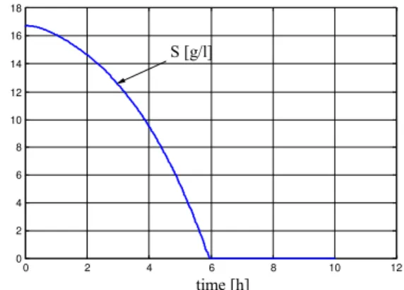
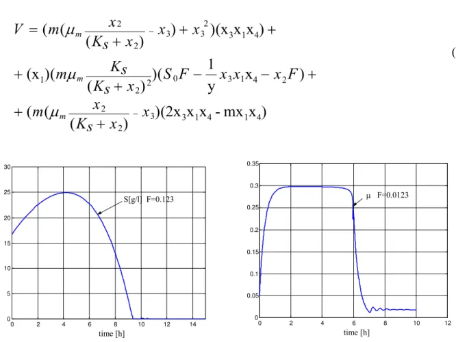
We optimise Jp=f(Fopt)= x1(T)x4(T) for a period of 10 hours ( KS=0.1 gl-1, µmax=0.3, S0=200

gl-1 ). The bioreactor volume V0 increases from 5 l. to 8 l.

Fig. 5 Optimal system: F=0.0523;(o) F=0.123 Fig. 6 Substrate concentration F=0.0123

From the Hamiltonian H(.) follows that the Fopt is maximum in the period [0 ÷Т] hours (max H). The control V of the model (22) is linked with F with the next formula:

y

Y

V

Y

2 2 3 3 4 2

1

Ψ

H

=

+

−

y Y Y

V Y

Y Y

2 .

4 .

3 3 .

2 2 .

1

− = = = =

0 2 4 6 8 10 12

0 2 4 6 8 10 12 14 16 18

(13)

)

x

mx

-x

x

(2x

)

(

)

x

y

1 (

)

(

)

(x

)

x

(x

)

(

4 1 4

1 3 3 2 2

2 4 1 3 0

2 2 1

4 1 3 2 3 3 2 2

x

s

K

x

m

F

x

F

S

x

s

K

s

K

m

x

s

K

x

m

V

m m m

− −

+

−

+

=

µ

0 2 4 6 8 10 12 14

0 5 10 15 20 25 30

time [h]

S[g/l] F=0.123

0 2 4 6 8 10 12

0 0.05 0.1 0.15 0.2 0.25 0.3 0.35

time [h]

µ F=0.0123

(24)

Fig. 7 Substrate concentration F=0.123 Fig. 8 Specific growth rate µ - F=0.0123

For model (1*) the optimal control is very simple F=Fmax (Fig 8, 9).

Fig. 9 Specific growth rate µ, F=0.223 Fig.10 Volume F=0.223

Direct application of the model (18) is the determination of some optimal control conditions

in order to reach the maximum Y4(T)=log(x1(T)x4(T)) in the end of the fed-batch process.

0 2 4 6 8 10 12 14 16

0 0.05 0.1 0.15 0.2 0.25 0.3 0.35

time [h]

µ

F = 0.223

0 2 4 6 8 10 12 14 16

5 5.5 6 6.5 7 7.5 8 8.5

(14)

(25)

The x3 is the specific growth rate. The maximum Y4(T) needs continuously maximum of the µ in the process period [0, T].

Conclusions

The Brunovsky normal form of the biotechnological models is very simple and the models are

linear with stationary coefficients. This form is convenient for optimization with the

Pontryagin maximum principle. Here all linear control theory is possible to be used without

restrictions. An advantage is the analytical determination of the optimal control laws like

functions of the parameters and the system state vectors. The main disadvantages of the

utilized approach are the complex formulas of the state vector Y, of the control V(U,x1,x2,x3)

and the difficult biotechnological interpretation.

The models (8 and 22) are linear and stationary. The diffeomorphic model (18) is simplified.

The tree first differentials equations are linear and stationary. This is of benefit to the control

practice.

References

1. Brunovsky P. (1970). A Classification of Linear Controllable Systems, Kibernetika,

v.3, pp.173-187.

2. Elkin V. (1999) Reduction of Non-linear Control Systems: A Differential Geometric

Approach – Mathematics and its Applications, v. 472, Handbound, Kluwer.

3. Gabassov R., Kirilova F. (1977). Optimization Methods. Minsk.

4. Hermann R. (1992). The GS Algorithm for Exact Linearization to Brunovsky Normal

Form. IEEE Trans. Aut. Contr., v.37, N2.

5. Pavlov Y. (2003). Equivalent models of fed-batch fermentation process and optimal

control, International Symposium and Young Scientists’ School BioPS’03, November

11-13, Sofia, pp. I.14 – I.17.

6. Pavlov Y. (2003). Equivalent Models of Fed-Batch Fermentation Process,

International Conference Automatics and Informatics’03, October 7– 8, Sofia, pp. 103

- 105.

µ

=

+

=

₂ ₃

1 1

2 .

4

)

(

Y

kY

x

(15)

7. Pavlov Y. (2001). Brunovsky Model for a Continuous Biotechnological Process,

International Conference Automatics and Informatics’01, June 7-9, Sofia, A-53 – A55.

8. Pavlov Y. (2001). Exact Linearization of a Non Linear Biotechnological Model

/Brunovsky Model/. Comptes Rendus de l'Academie Bulgares des Sciences, N 10, pp.

25-30.

9. Pavlov Y., St. Tzonkov. (2000). Kalman Filter and Continuos Biotechnological

Process Stabilisation: Peculiarities and Problems, International Symposium and

Young Scientists’ School BioPS’2000, pp. II 53- II 56 Sofia.

10.Pavlov Y., St. Tzonkov. (2000) Stabilization of a Specific Biotechnological Process:

Comparative Analysis, Technical ideas, N 3-4, , pp. 21-35.

11.Stanischkis and all. (1992). Automation biotechnological processes, automation

control, optimization and control, Riga, Sinatne.

12.Staphanopoulos G., K. San. (1984). Studies on On-Line Bioreactor Identification, I.

Biotechnol. & Bioeng., v. XXVI, pp. 1176-1188.

13.Tzonkov S., Filev D. and all. (1992). Control of biotechnological processes, Technika,

Sofia.

14. Wang T. W., Moore C., Birdwell D. (1987). Application of a Robust Multivariable

Controller to Non-linear Bacterial Growth Systems, Proceedings of the 10-th IFAC