www.atmos-meas-tech.net/9/5747/2016/ doi:10.5194/amt-9-5747-2016
© Author(s) 2016. CC Attribution 3.0 License.
Accuracy, precision, and temperature dependence of Pandora total
ozone measurements estimated from a comparison with the
Brewer triad in Toronto
Xiaoyi Zhao1, Vitali Fioletov2, Alexander Cede3,4, Jonathan Davies2, and Kimberly Strong1
1Department of Physics, University of Toronto, Toronto, M5S 1A7, Canada 2Environment and Climate Change Canada, Toronto, M3H 5T4, Canada 3NASA Goddard Space Flight Center, Greenbelt, MD 20771, USA 4LuftBlick, Kreith, Austria
Correspondence to:Xiaoyi Zhao ([email protected]) and Vitali Fioletov ([email protected]) Received: 27 July 2016 – Published in Atmos. Meas. Tech. Discuss.: 12 September 2016
Revised: 8 November 2016 – Accepted: 9 November 2016 – Published: 30 November 2016
Abstract. This study evaluates the performance of the re-cently developed Pandora spectrometer by comparing it with the Brewer reference triad. This triad was established by En-vironment and Climate Change Canada (ECCC) in the 1980s and is used to calibrate Brewer instruments around the world, ensuring high-quality total column ozone (TCO) measure-ments. To reduce stray light, the double Brewer instrument was introduced in 1992, and a new reference triad of double Brewers is also operational at Toronto. Since 2013, ECCC has deployed two Pandora spectrometers co-located with the old and new Brewer triads, making it possible to study the performance of three generations of ozone-monitoring in-struments. The statistical analysis of TCO records from these instruments indicates that the random uncertainty for the Brewer is below 0.6 %, while that for the Pandora is be-low 0.4 %. However, there is a 1 % seasonal difference and a 3 % bias between the standard Pandora and Brewer TCO data, which is related to the temperature dependence and dif-ference in ozone cross sections. A statistical model was de-veloped to remove this seasonal difference and bias. It was based on daily temperature profiles from the European Cen-tre for Medium-Range Weather Forecasts ERA-Interim data over Toronto and TCO from the Brewer reference triads. When the statistical model was used to correct Pandora data, the seasonal difference was reduced to 0.25 % and the bias was reduced to 0.04 %. Pandora instruments were also found to have low air mass dependence up to 81.6◦solar zenith an-gle, comparable to double Brewer instruments.
1 Introduction
Brewer) was introduced in 1992. The double Brewer has two spectrometers in series, significantly improving UV response and measuring global UV spectral irradiance, O3, SO2, and
aerosol optical depth. The double Brewer instruments also have a set of three instruments (serial numbers 145, 187, and 191) co-located with BrT to form the Brewer reference triad double (BrT-D). Individual Brewer instruments of the BrT and BrT-D are independently calibrated at Mauna Loa, Hawaii, every 2–6 years (Fioletov et al., 2005).
The Pandora system was developed at NASA’s Goddard Space Flight Center and first deployed in the field in 2006. Pandora instruments are based on a commercial spectrom-eter with stability and stray-light characteristics that make them suitable candidates for both direct-sun and zenith-sky measurements of total column ozone and other trace gases (Herman et al., 2009; Tzortziou et al., 2012). Pandora instru-ments have been tested and deployed in multiple scientific measurement campaigns around the world. These include the Cabauw Intercomparison Campaign of Nitrogen Diox-ide measuring Instruments (CINDI) in the Netherlands in 2009 (Roscoe et al., 2010) and four NASA DISCOVER-AQ campaigns since 2011 (Tzortziou et al., 2012). The Pan-dora instruments have been used for validation of satellite ozone (Tzortziou et al., 2012) and NO2(Herman et al., 2009;
Tzortziou et al., 2012) measurements. By 2015, several long-term Pandora sites had been established in the United States and worldwide (including Austria, Canada, the Canary Is-lands, Finland, and New Zealand). In 2013, two Pandora instruments (serial number 103 and 104) were deployed at Toronto co-located with BrT and BrT-D on the roof of the ECCC Downsview building (43.782◦N, 79.47◦W).
The instrument random uncertainties of BrT were anal-ysed by Kerr et al. (1996) and Fioletov et al. (2005) using similar methods. These methods both require knowledge of the extraterrestrial calibration (ETC) values, the ozone ab-sorption coefficients, and the Rayleigh scattering coefficients for each instrument. Fioletov et al. (2005) reported that the random uncertainties of individual observations from the BrT are within ±1 % in about 90 % of all measurements. This work takes a different approach, using a statistical variable estimation method to determine the random uncertainties for BrT, BrT-D, and the two Pandora instruments together. The variable estimation method follows the work of Fioletov et al. (2006) to estimate the random uncertainties with the as-sumption that there is no multiplicative bias between Pan-doras and Brewers. Details of the method are provided in Sect. 3.1. Since the instrument random uncertainties for BrT were last reported 10 years ago using data to 2004 (Fioletov et al., 2005), this work provides a new assessment of the per-formance of both the BrT and BrT-D in recent years, along with a comparison between coincident Brewer and Pandora measurements.
It is well known that the Dobson and Brewer ozone retrievals exhibit dependence on stratospheric temperature (Kerr et al., 1988; Redondas et al., 2014; Scarnato et al.,
2009). This is because the retrievals use different wave-lengths and ozone cross sections measured at fixed temper-atures. Brewer instruments have a very low temperature de-pendence (typically<0.1 % K−1) (Kerr et al., 1988; Kerr, 2002; Van Roozendael et al., 1998; Scarnato et al., 2009; Herman et al., 2015). For example, Kerr et al. (1988) reported a 0.07 % K−1temperature dependence for Brewer no. 8 (one of the BrT), and Kerr (2002) reported a 0.094 % K−1
tem-perature dependence for Brewer no. 14 (one of the BrT). In addition, Scarnato et al. (2009) reported that Brewer instru-ments (nos. 40, 72, and 156) exhibited less temperature de-pendence than Dobson instruments (nos. 83 and 101). Re-dondas et al. (2014) reported a 0.133 % K−1temperature
de-pendence for Dobson no. 83.
The Pandora ozone retrievals are more sensitive to strato-spheric temperatures. In Herman et al. (2015), the tempera-ture dependence for Pandora no. 34 (0.333 % K−1)was
de-termined by applying retrievals at a series of different ozone temperatures from 215 to 240 K for the ozone cross sections and then obtaining a linear fit to the percent change. As the small Brewer temperature dependence is known, we use co-incident measurements from the BrT and BrT-D to determine the temperature dependence factors for Pandora nos. 103 and 104, and then apply the correction to remove the dif-ference between Pandora and Brewer instruments.
2 Instruments and datasets 2.1 Pandora
The Pandora spectrometer system uses a temperature-stabilized (1◦C) symmetric Czerny–Turner system with a 50-micron entrance slit and 1200 lines mm−1 grating. Un-like the Brewer instruments, which only measure intensi-ties at selected wavelengths, the Pandora instruments, with a 2048×64 back-thinned Hamamatsu CCD detector, record spectra from 280 to 530 nm at 0.6 nm resolution (Herman et al., 2015). The spectra are analysed using the differential optical absorption spectroscopy (DOAS) technique (Noxon, 1975; Platt, 1994; Platt and Stutz, 2008; Solomon et al., 1987), in which absorption cross sections for multiple atmo-spheric absorbers (including ozone, NO2, SO2, HCHO, and
moved to the Canadian oil sands region in August 2014. Fol-lowing the work of Tzortziou et al. (2012), the Pandora ozone dataset is filtered to remove data from which the normalized root mean square (RMS) of weighted spectral fitting residu-als is greater than 0.05, and the Pandora-calculated standard uncertainty (Tzortziou et al., 2012) in TCO is greater than 2 DU.
2.2 Brewer
The Brewer instruments use a holographic grating in com-bination with a slit mask to select six channels in the UV (303.2, 306.3, 310.1, 313.5, 316.8, and 320 nm) to be de-tected by a photomultiplier. The first and second wavelengths are used for internal calibration and measuring SO2
respec-tively. The four longer wavelengths are used for the ozone re-trieval. The total column of ozone is calculated by analysing the relative intensities at these different wavelengths using the Bass and Paur (1985) ozone cross sections at a fixed ef-fective temperature of 228.3◦K (Kerr, 2002).
Most of the instruments in the BrT (nos. 8, 14, and 15) and BrT-D (no. 145, nos. 187, and 191) have been in operation since Pandora instruments were deployed. However, there are a few measurement gaps for some of the Brewers. For example, Brewers nos. 14 and 15 were recalibrated at Mauna Loa, Hawaii, in October 2013, and Brewer no. 145 was in Spain in March 2014 for an intercomparison. We also had to exclude some periods due to instrument malfunction and repairs. The coincident measurement periods for the instru-ments are shown in Table 1. The data from Brewer and Pan-dora instruments are both time-binned (3 min) for the com-parison. Following the work of Tzortziou et al. (2012), the Brewer dataset is filtered to remove data with calculated stan-dard uncertainty in TCO greater than 2 DU. In addition, the Brewer dataset is filtered for clouds by removing data for which the logarithm of the signal at 320 nm is less than the mean value minus 2 standard deviations (4 % of data were removed with this filter).
2.3 OMI
The Ozone Monitoring Instrument (OMI) is a nadir-viewing, near-UV–Vis spectrometer aboard NASA’s Earth Observ-ing System (EOS) Aura satellite (launched in July 2004). The OMI instrument measures the solar radiation backscat-tered by the Earth’s atmosphere and surface between 270 and 500 nm with a spectral resolution of about 0.5 nm (Lev-elt et al., 2006). The OMI TCO data are retrieved using both the Total Ozone Mapping Spectrometer (TOMS) tech-nique (developed by NASA (Bhartia and Wellemeyer, 2002) and based on a retrieval using four wavelengths at 313, 318, 331, and 360 nm) and the DOAS technique (developed by KNMI (Veefkind et al., 2006; Kroon et al., 2008) and based on the spectrum measured in the wavelength range 331.1–336.6 nm). The OMI TCO validation done by Balis
et al. (2007) shows a globally averaged agreement of bet-ter than 1 % for OMI–TOMS data and betbet-ter than 2 % for OMI–DOAS data in comparison with Brewer and Dobson measurements.
The OMI TCO products used in the present study are the Level-3 Aura/OMI daily global TCO gridded product (OMTO3e) retrieved by the enhanced TOMS Version 8 al-gorithm (Balis et al., 2007). The OMTO3e data (Bhartia, 2012) are generated by the NASA OMI science team by se-lecting the best pixel (shortest path length) data from the good-quality Level-2 TCO orbital swath data (for example, L2 observations with SZA<70◦; details can be found in Bhartia, 2012) that fall in the 0.25◦×0.25◦global grids. The OMTO3e data that come from the grid point over the ground-based site are used in this work to validate our correction method for Pandora TCO data.
2.4 ECMWF ERA-Interim data
In this work, the ozone-weighted effective temperature was used to assess the temperature sensitivity of Pandora ozone retrievals. Temperature and ozone profiles were extracted from the European Centre for Medium-Range Weather Fore-casts (ECMWF) ERA-Interim data for 2013–2015 (Dee et al., 2011) with 0.5◦×0.5◦ spatial resolution on 37 stan-dard pressure levels, available from http://apps.ecmwf.int/ datasets/. The ozone-weighted effective temperature (Teff)is
calculated based on daily ozone and temperature profiles (at 18:00 UTC) over Toronto, defined as
Teff= 30 X
i=6
weff,i·Ti, (1)
weff,i=
ni 30 P
j=6
nj
= MMRi·pi/Ti
30 P
j=6
MMRj·pj/Tj
, (2)
whereweff is the weighting function,Ti is the temperature,
ni is the ozone number density, MMRi is the ozone mass
mixing ratio, andpi is the pressure at pressure leveli. In this
work, profile data on ECMWF standard pressure levels from no. 6 to no. 30 (10–800 mbar) were used to decrease the noise from variable surface temperatures.
3 Statistical uncertainty estimation
Figure 1 shows the time series of the total column ozone datasets used in this work. The seasonal cycles of TCO from the ground-based and satellite instruments track each other well, and the high-frequency daily variations from all ground-based instruments are consistent.
Table 1.Coincident measurement periods and number of data points for comparisons between Pandora and Brewer instruments.
Pandora no. 103 Pandora no. 104
Brewer no. 8 Coincident period 18 Oct 2013–14 May 2015 20 Jan 2014–8 Aug 2014 Coincident data points 5008 2671
Brewer no. 14 Coincident period 25 Nov 2013–24 Dec 2015 16 Feb 2014–8 Aug 2014 Coincident data points 7797 1701
Brewer no. 15 Coincident period 31 Nov 2013–31 Jul 2014 20 Jan 2014–8 Aug 2014 Coincident data points 2297 1376
Brewer no. 145 Coincident period 15 Jan 2015–24 Dec 2015 N/A Coincident data points 1474 N/A
Brewer no. 187 Coincident period 18 Oct 2013–23 Apr 2014 20 Jan 2014–23 Apr 2014 Coincident data points 608 397
Brewer no. 191 Coincident period 20 Nov 2013–24 Dec 2015 21 Jan 2014–8 Aug 2014 Coincident data points 5359 1490
Figure 1. Ozone total column data from Pandoras, Brewers, and OMI:(a)Pandora nos. 103 and 104 compared with OMI–TOMS;
(b)Brewer triad (Brewer nos. 8, 14, and 15) compared with OMI– TOMS;(c)Brewer triad double (Brewer nos. 145, 187, and 191) compared with OMI–TOMS;(d)the daily mean difference, Brewer (or Pandora)–OMI.
about the random uncertainties can be derived from the mea-surements themselves (Grubbs, 1948; Toohey and Strong, 2007). The following method for doing this is described in Fioletov et al. (2006) and briefly explained below.
3.1 Method
We define the two types of measured TCO (denoted asMB
andMP, for Brewer and Pandora respectively) as simple
lin-ear functions of the true TCO value (X) and instrument ran-dom uncertainties (δB andδP), and assume that there is no
multiplicative or additive bias between Pandora and Brewer,
giving
MB=X+δB,
MP=X+δP. (3)
If we assume that the instrument random uncertainties are independent of the measured TCO, the variance ofMis the sum of the variances ofX (around the mean of the dataset) andδ:
σM2 B=σ
2 X+σδ2B, σM2
P=σ 2
X+σδ2P. (4)
If the difference between Pandora and Brewer does not de-pend onX (no multiplicative bias), and the random uncer-tainties of the two instruments are not correlated, then the variance of the difference is equal to the sum of the variance of the random uncertainties:
σM2
B−MP=σ 2 δB+σ
2
δP. (5)
Since we have the measured TCO and the difference between the Pandora and Brewer datasets, the variance of the TCO and instrument random uncertainties can be solved by
σX2=
σM2B+σM2P−σM2B−MP
/2,
σδ2B=
σM2B−σM2P+σM2B−MP
/2, (6)
σδ2P=
σM2P−σM2B+σM2B−MP
/2.
Equation (6) can be used to estimate the standard deviation (SD) of instrument random uncertainties (σδB andσδP)and the SD of ozone variability (σX). We do not actually know
the variancesσM2 i andσ
2
MB−MP; we can only estimate them, with some uncertainty, from the available measurements. It can be shown that the uncertainties in theσX2,σδ2
B, andσ 2 δP es-timates depend on the sum of all three variances (σM2
B,σ 2 MP, andσM2
itself is low (but one or more of the variancesσM2 B,σ
2 MP, and σM2
B−MP are high). The estimates are thus only as accurate as the least accurate of these parameters. The variance es-timates can be improved by increasing the number of data points or by reducing variances of Xby removing some of the daily variability. To remove the variability inX, the resid-ual ozone here is defined as the difference between the high-frequency TCO and the low-high-frequency TCO measured by an instrument:
dMres=Mhigh-f−Mlow-f. (7)
For example, the Brewer residual ozone could be the Brewer TCO measurements minus the Brewer ozone daily mean for that day, whereas the corresponding Pandora residual ozone would be the Pandora TCO measurements minus the Pandora ozone daily mean. By subtracting the low-frequency signal, we remove most of the ozone variability. In addition, as pro-posed in Fioletov et al. (2005), to improve the removal of the bias, we can use the following statistical model to calculate the low-frequency signal:
Mlow-f=AB·IB+AP·IP+B·(t−t0)+C·(t−t0)2, (8)
wheret is the time of the measurement andt0is the time of
local solar noon.IBis an indicator function for the Brewer
in-strument; it is set to 1 if the TCO is measured by the Brewer and to 0 otherwise.IP is the indicator function for the
Pan-dora. The coefficients AB,AP,B, andC are estimated by
the least-squares method for each day (for example, the cal-culated low-frequency signal for Brewer and Pandora will share the sameB andC terms, but they have their own off-setsABandAP). In the following, we will refer to the
resid-ual ozone calculated by subtracting the daily mean value as residual type 1 and that obtained by subtracting this second-order function as residual type 2. The present work is focused on evaluating the high-quality TCO data. Thus to avoid the stray-light effect, in the statistical uncertainty estimation, we only use Pandora and Brewer data with ozone air mass fac-tor (AMF) less than 3 (see Sect. 4 for more details about the stray-light effect).
3.2 Results
In this work, we calculate two different types of residual ozone (see Eq. 7) as defined in Sect. 3.1 and then use them to calculate the instrument random uncertainty with the sta-tistical variable estimation method (Eq. 6; more details can be found in Fioletov et al., 2006). For example, we use Eqs. (7) and (8) to calculate two type 2 residuals for both Brewer and Pandora (dMb-res2 and dMp-res2), and then
cal-culate their difference (dMb-res2−dMp-res2). Next, we
calcu-late their variances values σ2(dMb-res2), σ2(dMp-res2), and
σ2(dMb-res2−dMp-res2). Those variance terms are used in
Eq. (6) to estimate the random uncertainties. The residual types and relevant terminologies are summarized in Table 2.
Table 2.Definition of terminologies used in the uncertainty estima-tion.
Definition
Estimated random uncertainty (σδ)
Random uncertainty estimated using the statistical variable estimation method described in Sect. 3.1
Mhigh-f High-frequency TCO
measure-ments, averaged in 3 min bin Mlow-f (daily mean) Low-frequency TCO,
calculated as the daily mean TCO
Mlow-f (2nd order function) Low-frequency TCO,
calculated using the second-order function (Eq. 8)
Residual type 1 Mhigh-f−Mlow-f (daily mean) Residual type 2 Mhigh-f−
Mlow-f (2nd order function)
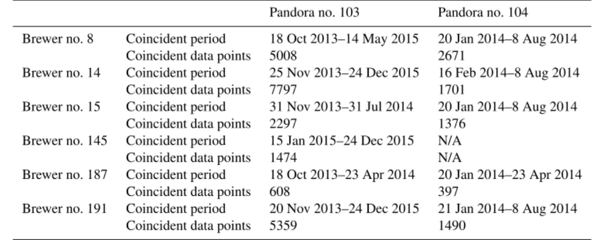
Figure 2.Estimated random uncertainties: for the Brewer instru-ments using(a)residual ozone type 1 and(b)residual ozone type 2; for the Pandora instruments using(c)residual ozone type 1 and
(d) residual ozone type 2. The black squares indicate data from Pandora no. 103, and the red triangles indicate data from Pandora no. 104. The error bars show the 95 % confidence bounds.
Figure 2 shows the Brewer-estimated random uncertainties obtained using the two types of residual ozone data (Fig. 2a for residual type 1, Fig. 2b for type 2). For example, in Fig. 2a, the estimated random uncertainty for Brewer no. 8 using Pandora no. 103 data (residual type 1, derived from MP103)is shown as a black square in the column for Brewer no. 8, while its estimated random uncertainty using Pandora no. 104 data (residual type 1, derived fromMP104)is shown as a red triangle in the same column. Figure 2 demonstrates that type 1 (Fig. 2a) and type 2 (Fig. 2b) residual ozone data provide comparable results and confirm that Brewer instru-ments have random uncertainties of 1–2 DU.
Figure 3.Estimated residual ozone variability (σX)using(a) resid-ual ozone type 1 and(b)residual ozone type 2.(c)Number of coin-cident measurements used in the statistical uncertainty estimation. The black squares indicate data from Pandora no. 103, and the red triangles indicate data from Pandora no. 104. The error bars show the 95 % confidence bounds.
the estimated random uncertainty for Pandora no. 103 us-ing Brewer no. 8 data is shown as a black square in the col-umn of Brewer no. 8, while its estimated random uncertain-ties using other Brewer data are shown by respective Brewer columns. Figure 2 demonstrates that the Pandora instruments have estimated random uncertainties less than 1.5 DU. Slight differences in the estimated Pandora random uncertainties were found using different Brewer instruments. This is due to the sample size; when the sample size is large (>1200 coincident points; see Table 1), the Pandora-estimated ran-dom uncertainties from different instruments are more con-sistent. For example, in Fig. 2c, one of the estimated random uncertainties for Pandora no. 103 (black square in Brewer no. 187 column) is below 0.5 DU. This result is undesirable (the value is ∼0.5 DU lower than the other values) but not
unusual. Dunn (2009) describes this issue in detail and points out that the low (even negative in some cases) variance esti-mate is due to small sample size. In general, Dunn (2009) concludes that, even with the correct model, the comparisons and estimation of precision are only viable with large sam-ple sizes. Figure 3c shows that the low variance was indeed from the smallest sample size (608 coincident points for Pan-dora no. 103 vs. Brewer no. 187 and 397 for PanPan-dora no. 104 vs. Brewer no. 187). In addition, when using the data from the same pair of Brewer and Pandora instruments, the esti-mated random uncertainty for Pandora is consistently lower than that for Brewer by∼0.5 DU.
Fioletov et al. (2006) estimated natural ozone variability (σX)using Eq. (6). However, because we are using the
resid-ual ozone instead of the TCO in the statistical analysis, the σX calculated from our method is not the estimated natural
ozone variability but the estimated residual ozone variabil-ity for the measurement period. It can be used to character-ize the difference between residual types 1 and 2. Figure 3a
Figure 4.Scatter plots for residual ozone type 1 and 2, colour-coded by the normalized density of the points.(a)Brewer no. 8 vs. Pan-dora no. 103 (residual type 1),(b)Brewer no. 8 vs. Pandora no. 104 (residual type 1),(c)Brewer no. 8 vs. Pandora no. 103 (residual type 2),(d)Brewer no. 8 vs. Pandora no. 104 (residual type 2). The black line is the one-to-one line.
shows the estimated residual ozone variability using residual type 1 data, while Fig. 3b shows the variability using residual type 2. Figure 3a and b demonstrate that residual type 1 data have larger variability than type 2 data, indicating that us-ing the daily mean value as the low-frequency signal did not fully remove the natural ozone variability. Ideally, the ran-dom uncertainty estimate should only contain ranran-dom noise caused by the instrument and no natural ozone variation. Scatter plots of Brewer vs. Pandora residual ozone (Fig. 4) illustrate the same results. Figure 4 shows that the correla-tion coefficients for residual type 1 (R=0.813 for Brewer
no. 8 vs. Pandora no. 103, see Fig. 4a; 0.909 for Brewer no. 8 vs. Pandora no. 104, see Fig. 4b) are higher than the ones for residual type 2 (0.333 for Brewer no. 8 vs. Pandora no. 103, see Fig. 4c; 0.688 for Brewer no. 8 vs. Pandora no. 104, see Fig. 4d). The low correlation coefficients for ozone residual type 2 data indicate that the ozone variability has been largely removed from Pandora and Brewer data. Thus when we use residual ozone type 2, even with relatively small sample size, the estimated uncertainties for Pandoras are still consistent with those obtained from comparisons with other Brewers having larger sample sizes (see Fig. 2c and d, Brewer no. 187 column).
Figure 5. Time series of Brewer no. 14–Pandora no. 103 TCO difference colour-coded by ozone effective temperature (see Eq. 1): (a) before applying the temperature dependence correc-tion and (b) after applying the correction. The dashed lines are LOWESS(0.5) fits.
showing the consistency of results from both type 1 and 2 in Fig. 2, we validated the use of the second-order statistical model (Eq. 8) and proved some of the advantages when us-ing type 2. For example, the residual type 2 could work with smaller data size than the residual type 1 (without making the estimated variance unrealistic, too low, or even negative). In general, Fig. 2 demonstrates that the Pandora TCO data have
∼0.5 DU smaller estimated random uncertainties than the Brewer TCO data. The mean estimated random uncertainties for BrT and BrT-D are in the range of 1–2 DU (∼0.6 %). The mean estimated random uncertainties for Pandora nos. 103 and 104 are in the range of 0.5–1.5 DU (∼0.4 %). These re-sults confirm the quality of the TCO data, with all eight in-struments meeting the GAW requirement for a precision bet-ter than 1 % to measure ozone (WMO, 2014).
4 Temperature dependence effect and correction 4.1 Method
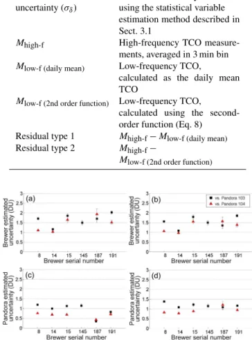
When comparing Pandora and Brewer TCO data, we can see a clear seasonal structure and a bias in the difference and ratio. Figure 5a shows the time series of Brewer no. 14– Pandora no. 103 TCO difference; the seasonal amplitude is 3–4 DU, and the mean bias is 10.81 DU. Figure 5b (which
Figure 6. Linear regression of Brewer/Pandora TCO ratio as a function of effective temperature minus 225 K.(a)Linear regres-sion results;(b)residual plot of the linear regression.
uses the corrected data) will be discussed in Sect. 4.2. The locally weighted scatter plot smoothing (LOWESS(x)) fit (the dashed line) is based on local least-squares fitting ap-plied to a specified x fraction of the data (Cleveland and Devlin, 1988). The bias between Pandora and Brewer TCO is mainly due to the fact that both retrievals depend on the choice of ozone absorption cross section (Scarnato et al., 2009; Herman et al., 2015). The Brewer TCO in this work was retrieved using the standard Brewer network operational ozone cross section (Bass and Paur, 1985), while the Pandora TCO was retrieved using the standard Pandora network oper-ational ozone cross section (the DBM ozone cross section). Redondas et al. (2014) reported that changing the Brewer op-erational ozone cross section from Bass and Paur (1985) to that of Daumont et al. (1992) (DBM) will change the calcu-lated TCO by−3.2 %. In addition to the offset caused by the use of different ozone cross sections, the seasonal difference between Pandora and Brewer TCO data is due to their differ-ing temperature dependence, which varies from instrument to instrument because of the differences in ozone retrieval al-gorithm and instrument design. Moreover, even for the same type of instrument, the temperature sensitivity can be differ-ent due to imperfections in the wavelength settings and slit function for each individual instrument. We will study these differences (offset and temperature effect) by using the stan-dard TCO products from Pandora and Brewer instruments.
In this work, we use ECMWF ERA-Interim ozone and temperature profiles to calculate daily ozone effective tem-perature (described in Sect. 2.4). Then we use the following simple linear regression model to find the temperature depen-dence factor for Pandora instruments:
MB
MP
whereais the temperature dependence factor for Pandora,b is the (systematic) multiplicative bias between Pandora and Brewer, and 225 refers to effective temperature of 225◦K for ozone cross sections used in the Pandora retrievals. Here, the MBandMP are TCO daily means measured by the Brewer
and Pandora respectively. To increase the number of coin-cident data points, theMBdataset is formed by merging all
measurements from the six Brewers (see Table 1). A success-fully merged MB data point has coincident measurements
from at least two Brewers, to avoid domination by a single instrument. The coincident time period of theMBandMP103
datasets is from October 2013 to December 2015 with 272 coincident days (points). Figure 6 shows the linear regres-sion results for Pandoras nos. 103 and 104. We found the “relative temperature dependence factor” (RTDF) for Pan-dora no. 103 to be 0.247±0.013 % K−1(from the term a
in Eq. 9), with a 2.2±0.1 % multiplicative bias (from the term b in Eq. 9). Although Pandora no. 104 only has mea-surements from January to April 2014 (53 coincident days), the linear regression still results in a similar temperature de-pendence factor (0.255±0.040 % K−1)and the same bias as Pandora no. 103. The correlation coefficients for those two linear regressions are 0.91 and 0.89 respectively.
We applied the Pandora temperature dependence factors to the Pandora TCO to remove its bias and seasonal difference relative to Brewer TCO data. Similar to the correction func-tion used in Herman et al. (2015) for Pandora no. 34, we used the following function to correct Pandora TCO data: Mcorr=MP·(a·(Teff−225)+b) , (10)
whereMcorr is corrected Pandora TCO, and other terms are as defined for Eq. (9). For the Pandora no. 103 dataset, this becomes
Mcorr=MP103·(0.00247·(Teff−225)+1.022) , (11)
where MP103 is the TCO data from Pandora no. 103. The
temperature dependence factor (0.247±0.013 % K−1) and
the multiplicative bias (1.022) are found in Fig. 6. The same regression model and method give a 0.255±0.040 % K−1
temperature dependence factor with a 2 % multiplicative bias to Pandora no. 104, and hence
Mcorr=MP104·(0.00255·(Teff−225)+1.022) , (12)
whereMP104 is the Pandora no. 104 TCO. For comparison, Herman et al. (2015) derived the correction function for Pan-dora no. 34 as
Mcorr=MP34·(0.00333·(Teff−225)+1) , (13)
where the 0.00333 (0.333 % K−1)is the temperature depen-dence factor for Pandora no. 34. Note that this value was de-termined by applying retrievals using ozone cross sections from 215 to 240 K and then obtaining a linear fit to the per-cent change (Herman et al., 2015). However in this work, the
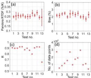
Figure 7.Pandora relative temperature dependence factors derived from 13 sensitivity tests (shown in Table 3).(a)RTDFs,(b) multi-plicative biases,(c)correlation coefficients (R), and(d)number of data points in sensitivity tests. The error bars show the 95 % confi-dence bounds.
factors for Pandora nos. 103 and 104 were found by statis-tical analysis (comparison) of the Pandora and Brewer TCO datasets. Thus our temperature dependence factor combines the temperature sensitivity from both Pandora and Brewer in-struments, and describes the relative temperature sensitivity between the Pandora and Brewer standard TCO products. We call it a “relative temperature dependence factor” (RTDF), while that from Herman et al. (2015) is an absolute tem-perature dependence factor (ATDF). Although the RTDF is a non-linear combination of ATDF from both Pandora and Brewer (note that the Pandora used an ozone cross section at an effective temperature of 225 K, while the Brewer used that at 223.8 K), we can still make a simple linear estima-tion of the RTDF from reported ATDFs. In fact, the reported ATDF for Pandora no. 34 (0.333 % K−1; Herman et al., 2015)
minus the reported ATDF for Brewer nos. 8 and 14 (0.07 and 0.094 % K−1; Kerr et al., 1988; Kerr, 2002) gives
rel-ative numbers (0.26 and 0.24 % K−1) that are close to our
model-calculated RTDF (∼0.25 % K−1). In our correction
functions (Eqs. 11–12), we have a constantbterm of 1.022 given 0.001 uncertainty, which indicates a multiplicative bias of∼2 % (not caused by the temperature effect) between the Pandora and Brewer instruments due to their different selec-tion of ozone cross secselec-tions.
Table 3.Summary of sensitivity tests for Pandora relative temperature dependence factors.
Test no. Pandora Brewer Data period RTDF (% K−1)
1 no. 103 Combined Brewer (no. 8, no. 14, no. 15, no. 145, no. 187, no. 191) Oct 2013–Dec 2015 0.247±0.013 2 no. 104 Combined Brewer (no. 8, no. 14, no. 15, no. 187, no. 191) Jan 2014–Apr 2014 0.255±0.040 3 no. 103 Combined Brewer (no. 8, no. 14, no. 15, no. 187, no. 191) Jan 2014–Apr 2014 0.261±0.027 4 no. 103 Combined Brewer (no. 8, no. 14, no. 15, no. 187, no. 191) Oct 2013–Aug 2014 0.255±0.020 5 no. 103 Combined Brewer (no. 8, no. 14, no. 145, no. 191) Jan 2015–Dec 2015 0.263±0.017
6 no. 103 Brewer no. 191 Oct 2013–Dec 2015 0.246±0.016
7 no. 103 Brewer no. 191 Oct 2013–Aug 2014 0.249±0.025
8 no. 103 Brewer no. 191 Jan 2015–Dec 2015 0.250±0.021
9 no. 103 Brewer no. 8 Oct 2013–May 2015 0.285±0.031
10 no. 103 Brewer no. 14 Nov 2013–Dec 2015 0.262±0.014
11 no. 103 Brewer no. 15 Nov 2013–Jul 2015 0.290±0.025
12 no. 103 Brewer no. 145 Jan 2015–Dec 2015 0.241±0.020
13 no. 103 Brewer no. 187 Oct 2013–Apr 2014 0.242±0.088
to the small data size, the RTDF for test 2 has larger error bars than test 1. Test 3 shows Pandora no. 103 RTDF using combined Brewer data for the same time period as Pandora no. 104. Pandora no. 103 has a measurement gap from Au-gust to December 2014 due to instrument failure (see Fig. 1); hence, tests 4 and 5 use combined Brewer data for 2013– 2014 (∼1-year coverage, before the instrument failure of
Pandora no. 103) and 2015 (1-year coverage, after Pandora no. 103 was repaired) separately. Brewer no. 191 was one of the most reliable Brewer instruments during the compar-ison period. Thus tests 6–8 use only Brewer no. 191 data; test 6 uses all available data (2013–2015), test 7 uses only 2013–2014 data (before the instrument failure of Pandora no. 103), and test 8 uses 2015 data (after Pandora no. 103 was repaired). Tests 9–13 use individual Brewer data (all avail-able data for each individual Brewer). For the 13 tests, the RTDFs (see Fig. 7a) are in the range of 0.24–2.9 %, and the multiplicative biases (see Fig. 7b) are in the range of 1.7– 2.5 %. The correlation coefficients (see Fig. 7c) for most tests are above 0.8. In general, the RTDFs found for the Pandora instruments are stable when derived from combined Brewer data or reliable individual Brewer data. For this 2-year data period, the derived RTDFs from BrT-D instruments are lower (0.241–0.246 % K−1) than the ones from BrT instruments
(0.262–0.290 % K−1). However, with the large uncertainties
on the estimated RTDFs and the bias, we could not conclude whether this is due to the different instrument designs or a sampling issue.
5 Results
5.1 Pandora TCO correction
As an example, Fig. 5 shows the time series of Brewer no. 14–Pandora no. 103 TCO differences, before and after applying the Pandora correction (Eq. 11). A clear seasonal signal is seen due to the variation of Teff before we apply
Figure 8.Scatter plots of Pandora no. 103 vs. Brewer no. 14 TCO, colour-coded by ozone effective temperature:(a)before applying the correction and(b) after applying the correction. The red line is a simple linear fit, the green line is the linear fit weighted by the calculated standard uncertainty from Pandora and Brewer TCO data, the blue line is the linear fit with intercept set to 0, and the black line is the one-to-one line.
Figure 9. Effective ozone temperature:(a) Teff calculated using ECMWF ERA-Interim data (18:00 UTC over Toronto) and NASA climatology data (monthly mean for 40–50◦N), and(b)the differ-ence between these two.
slope of 0.969, indicating−3.1 % mean bias. This is consis-tent with the work of Redondas et al. (2014), which showed that changing the Brewer ozone cross section from Bass and Paur to DBM changed the Brewer TCO by −3.2 %.
By colour coding the scatter points, it is obvious that this non-ideal slope and offset are related toTeff. After applying
the correction, the seasonal Brewer–Pandora difference dis-appears as seen in Fig. 5b, and the linear regression (green line) gives a slope of 1.008, an offset of−2.678 DU, and an improved correlation (R=0.9982) (see Fig. 8b). Linear fit-ting with zero intercept gives a slope of 1.001, indicafit-ting that the correction improves the mean bias between Pandora and Brewer TCO from−3.1 to 0.1 %.
To calculate the effective temperature, we use daily tem-perature and ozone profiles from ECMWF ERA-Interim data at 18:00 UTC for Toronto, but Herman et al. (2015) used monthly averaged temperature and ozone climatology data (interpolating the climatological ozone profile to the ob-served TCO in order to capture day-to-day variability; see ftp://toms.gsfc.nasa.gov/pub/ML_climatology) for latitudes of 30–40 and 40–50◦N to form an average suitable for Boul-der (40◦N). To understand the difference due to the selection of Teff, we adapted the climatology data used in Herman et
al. (2015) and used the data from 40 to 50◦N to calculate effective ozone temperature for Toronto (44◦N). Figure 9 shows the comparison between the ECMWF daily Teff and
the NASA monthly climatologyTeff. A sudden cooling event
happened at Toronto on 29–30 January 2014, for which the difference between the daily and monthly Teff was−10 K. Figure 10 shows the time series of TCO difference (com-bined Brewer–Pandora no. 103) before and after applying the temperature dependence correction using both the monthly climatologyTeffand dailyTeff. Because the monthly
clima-tologyTeffdoes not reflect the low temperature during those
two days, the correction function (see Eq. 11) overcompen-sated for the temperature effect (the minimum delta ozone value on 29 January changed from −8 DU in Fig. 10a to
−14 DU in Fig. 10b). The low-temperature event was
cap-Figure 10.Time series of combined Brewer–Pandora no. 103 TCO difference colour-coded by ozone effective temperature:(a)before applying the temperature dependence correction,(b)after applying the correction using NASA monthly climatologyTeff, and(c)after applying the correction using ECMWF EAR-Interim dailyTeff. The sudden cooling event on 29–30 January 2014 is marked by a black box. The dashed lines are LOWESS(0.5) fits.
tured by the dailyTeff; thus the compensation from the
tem-perature effect was reasonably small when using ECMWF daily Teff (the minimum value was −7 DU; see Fig. 10c).
In general, the ECMWF dailyTeff can better capture some
ozone variation events that are associated with rapid temper-ature changes.
Figure 11. Monthly mean time series of the (Brewer−Pandora)/Brewer % TCO difference: (a) before applying the Pandora temperature dependence correction and
(b)after applying the correction. The shaded regions represent 1σ uncertainty.
applying the TCO corrections (Fig. 11b), the seasonal differ-ences decreased from±1.02 to±0.25 % for Pandora no. 103
and from±0.40 to±0.25 % for Pandora no. 104, as did the offset which decreased from 2.92 to −0.04 % for Pandora no. 103 and from 2.11 to−0.01 % for Pandora no. 104. The 1σ uncertainty in Fig. 11b shows that, statistically, the cor-rected Pandora datasets have no significant seasonal differ-ences or offsets compared to the Brewer datasets.
5.1.1 Comparison with OMI
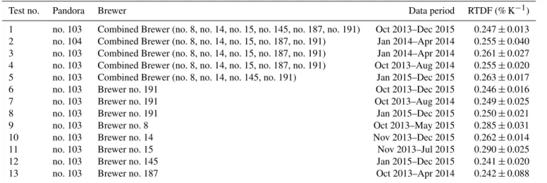
To further validate the temperature dependence correction for the Pandora data, we used OMI ozone data (version OMTO3e). Pandora data are averaged within ±10 min of OMI overpass times. In Fig. 12, scatter plots of OMI vs. Pandora TCO are shown in panels a and b; OMI vs. cor-rected Pandora TCO (using Eqs. 11 and 12 with the correc-tion funccorrec-tions found from our statistical model) is shown in panels c and d; and OMI vs. corrected Pandora TCO (us-ing Eq. 13 with the correction function from Herman et al., 2015) is shown in panels e and f. All the Pandora TCO cor-rections shown in Fig. 12 used the sameTeffcalculated with the ECMWF ERA-Interim daily ozone data.
Figure 12a and c show that, after applying the TCO cor-rection (Eq. 11) to Pandora no. 103, the slope of the lin-ear regression improved from 0.987 to 0.990, the offset im-proved from 14.84 to−3.59 DU, the correlation coefficient improved from 0.987 to 0.991, and the mean bias between
Figure 12.Scatter plots of OMI TCO vs. Pandora TCO for(a) Pan-dora no. 103 without TCO correction,(b)Pandora no. 104 without TCO correction,(c)Pandora no. 103 with correction using Eq. (11),
(d)Pandora no. 104 with correction using Eq. (12), (e)Pandora no. 103 with correction using Eq. (13), and(f)Pandora no. 104 with correction using Eq. (13).
OMI and Pandora improved from 3.1 to 0.02 %. Similar improvement is seen in the comparison between Pandora no. 104 and OMI (see Fig. 12b and d), although the size of the coincident measurement dataset is smaller, with the mean bias improving from 1.5 to −0.6 %. In addition, Fig. 12e
and f show that, by using the correction function from Her-man et al. (2015), the comparisons also improve, although 1.9 % (1.4 %) bias remains for Pandora no. 103 (no. 104) (in-dicated by the slop of linear fit with force the intercept to 0; see the green lines in Fig. 12). Note that the ATDF in Herman et al. (2015) is only 0.08 % K−1higher than our RTDF.
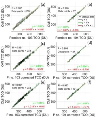
Figure 13a and b shows the monthly mean time series of the OMI–Pandora TCO percentage difference, before and after applying the three correction functions. All three cor-rection models reduced the difference between Pandora and OMI. Our relative correction model (Eqs. 11 and 12) reduces the seasonal difference (indicated by the δ of the percent-age monthly delta ozone) between Pandora no. 103 and OMI from±1.68 to±1.00 %, with the mean bias decreasing from
2.65 to−0.19 % (the mean of the percentage monthly delta
Figure 13. Monthly mean time series of the (OMI−Pandora)/OMI % TCO difference:(a)before applying the correction,(b)after applying the correction using Eqs. (11)–(13), and(c)the difference between the corrections. The shaded regions represent the 1σuncertainty.
mean bias between Pandora and OMI is better for the relative correction model. This result (−0.19±1.00 % mean bias) is consistent with Balis et al. (2007), who showed that the global average difference between OMI–TOMS and Brewer instruments is within 0.6 %, and that the difference in the 40–50◦N band (Toronto is at 44◦N) is close to 0 (see their Fig. 1).
Balis et al. (2007) reported that the time series of glob-ally averaged differences between OMI–TOMS and Brewer instruments shows almost no annual variation, and the OMI– TOMS data theoretically have no temperature dependence (McPeters and Labow, 1996; Bhartia and Wellemeyer, 2002). By using our relative correction, the corrected Pandora TCO should have similar performance to the Brewer TCO. Fig-ure 13c shows the difference between the absolute correction method and the relative correction method. Although both methods removed some of the seasonal signal (reduced from
1.68 to 1.00 % for the relative correction and to 0.87 % for the absolute correction), Fig. 13c shows that there is still a weak seasonal signal residual (0.39 %) left between these two methods.
6 Stray-light effect
It is well known that direct-sun UV spectrometers are af-fected by stray light when the solar zenith angle (SZA) is too large. In general, when the ozone AMF is larger than 3 (SZA>70◦), the retrieved TCO will show an unrealis-tic decrease with increasing SZA (thus this effect is also known as the air mass dependence effect). In general, the stray light from longer wavelengths results in overestimation of the UV signal at short wavelengths and makes the mea-sured UV signal in that part of the spectrum less sensitive to TCO. The double Brewer spectrometer was introduced in 1992, which uses two spectrometers in series to reduce the stray light (Bais et al., 1996; Wardle et al., 1996; Fioletov et al., 2000). The BrT-D has the advantage of very low internal stray-light fraction (10−7, stray-light signal divided by total
signal) compared to BrT (10−5)in the 300–330 nm spectral
range (Fioletov et al., 2000; Tzortziou et al., 2012). For Pan-dora instruments, a UV340 filter is used to remove most of the stray light that originates from wavelengths longer than 380 nm (Herman et al., 2015). A typical UV340 filter has a small leakage (5 %) at∼720 nm, which misses the detector and hits the internal baffles. Further stray-light correction is done by subtracting the signal of pixels corresponding to 280 to 285 nm (which contain almost zero direct illumination) from the rest of the spectrum. However, a very small (but unknown) amount of this stray light may scatter onto the de-tector (Herman et al., 2015). Tzortziou et al. (2012) tested the stray-light effect for Pandora no. 34 and Brewer no. 171 and concluded that the Pandora stray-light fraction (∼10−5)was comparable to the single Brewer. Pandora ozone retrievals are accurate up to a slant column between 1400 and 1500 DU or 70 and 80◦SZA, depending on the TCO amount (Herman et al., 2015).
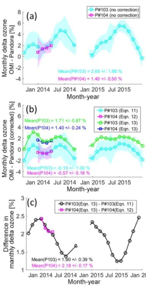
In this work, to assess the air mass dependence, we com-pared Brewer TCO to the corrected Pandora TCO data. Fig-ure 14 shows an example of the Brewer/Pandora ratio as a function of ozone AMF (reported value in Brewer data) be-fore and after applying the TCO correction (Eq. 11), with the data points grouped by effective temperature. Before ap-plying the correction (Fig. 14a), the linear fits show con-sistently low (−0.1 to 0.5 %) relative AMF dependence be-tween Brewer and Pandora (defined as the slope of the linear fit) for eachTeff group. However, the linear fit to the whole
Figure 14.Brewer no. 14/Pandora no. 103 TCO ratio vs. ozone air mass factor:(a)before and(b)after applying the Pandora temper-ature dependence correction. The points are grouped by effective temperature (from 215 to 240 K, in 5 K bins), and the linear fits for each group are colour-coded. The black line and linear fit are for the whole dataset.
Figure 15. Percentage difference between Pandoras (nos. 103 and 104) and Brewers (grouped as BrT and BrT-D) as a function of ozone air mass factor. On each box, the central mark is the me-dian, the edges of the box are the 25th and 75th percentiles, and the whiskers extend to the most extreme data points not considered outliers.
To characterize only the air mass dependence, we therefore removed the temperature dependence effect from the Pan-dora dataset.
To show how the different instrument designs affect the stray-light performance, we merged the six Brewer datasets into two groups (BrT and BrT-D) to compare
with the corrected Pandora data. Figure 15 shows the (Brewer−Pandora)/Brewer percentage difference as a function of ozone AMF. In Sects. 3 and 4, the TCO data with ozone AMF>3 were discarded. The purpose of this fil-ter was to ensure that only the best direct-sun measurements (with low air mass dependence) from both instruments were used. However, to study the instrument performance for large AMFs, and also to characterize the performance of Brewer and Pandora instruments, we changed the AMF threshold from 3 to 6. Figure 15 indicates that Pandora, BrT, and BrT-D instruments have similar air mass dependence for ozone AMF<3 (∼71◦ SZA), consistent with the result reported by Tzortziou et al. (2012). Pandora and BrT-D have similar AMF dependence up to ozone AMF of 5.5–6 (80.6–81.6◦ SZA), but Pandora and BrT diverge above AMF of 3–4 (71– 76◦SZA). In general, these results indicate the Pandora and BrT-D instruments have very good stray-light control.
7 Conclusions
The instrument random uncertainty, TCO temperature pendence, and ozone air mass dependence have been de-termined using two Pandora and six Brewer instruments. In general, Pandora and Brewer instruments both have very low random uncertainty (<2 DU) in the total column ozone mea-surements, with that for Pandora being∼0.5 DU lower than Brewer. This indicates that Pandora instruments could pro-vide more precise measurements than the Brewer for the study of small-scale (temporal and magnitude) atmospheric changes. This work confirms the quality of the TCO data, with all eight instruments meeting the GAW requirement for a precision better than 1 % (WMO, 2014); however, the Brewer instruments have smaller ozone temperature depen-dence than the Pandoras.
By using the ECMWF ERA-Interim and Brewer ozone data in the statistical method, we successfully corrected the Pandora TCO to decrease its temperature depen-dence. We found relative temperature dependence factors of 0.247 % K−1for Pandora no. 103 and 0.255 % K−1for
Pan-dora no. 104 against the Brewer instruments. This relative temperature dependence factor is comparable to the abso-lute temperature dependence factors previously found for Pandora (0.333 % K−1, by applying retrievals with
differ-ent ozone cross sections, Herman et al., 2015) and Brewers (0.07–0.094 % K−1; Kerr et al., 1988; Kerr, 2002). In
addi-tion, a 2 % multiplicative bias was found between the Pan-dora and Brewer standard TCO products, which is due to the different ozone cross sections used in the retrievals. Af-ter applying the corrections, the annual seasonal difference between Pandora and Brewer instruments decreased from
Pan-dora measurements (Kerr, 2002; Tiefengraber et al., 2016), albeit at a cost of decreased TCO measurement precision. An effective ozone temperature algorithm is under development for the Pandora. The future operational Pandora ozone re-trieval algorithm will use this derived effective ozone temper-ature to minimize the tempertemper-ature dependence of the ozone product (Tiefengraber et al., 2016).
This study confirmed that the Pandora and Brewer TCO data have negligible air mass dependence when the ozone AMF<3. The Pandora and BrT instruments have similar air mass dependence (relative air mass dependence<±0.1 %) up to 71◦ SZA (AMF<3); the Pandora and BrT-D instru-ments have very good stray-light control, and their AMF de-pendence is comparably low up to 81.6◦SZA (within 1 % up to AMF=5.5 and within 1.5 % up to AMF=6).
8 Data availability
Data from the BrT, BrT-D, and Pandora instruments are available through Environment and Climate Change Canada (contact Vitali Fioletov, [email protected]). The final version of the Brewer data is (or will be) available from the World Ozone and UV Data Centre (doi:10.14287/10000001). OMTO3e data are available from the GES DISC: doi:10.5067/Aura/OMI/DATA3002 (GES DISC, 2004). Any additional data may be obtained from Xi-aoyi Zhao ([email protected]).
Acknowledgements. X. Zhao was partially supported by the
NSERC CREATE Training Program in Arctic Atmospheric Science. We thank ECMWF for providing the ERA-Interim model data and the NASA OMI ozone retrieval team for providing the OMTO3e data.
Edited by: M. Van Roozendael Reviewed by: three anonymous referees
References
Bais, A., Zerefos, C., and McElroy, C.: Solar UVB measurements with the double-and single-monochromator Brewer ozone spec-trophotometers, Geophys. Res. Lett., 23, 833–836, 1996. Balis, D., Kroon, M., Koukouli, M., Brinksma, E., Labow, G.,
Veefkind, J., and McPeters, R.: Validation of Ozone Monitoring Instrument total ozone column measurements using Brewer and Dobson spectrophotometer ground-based observations, J. Geo-phys. Res., 112, D24S46, doi:10.1029/2007JD008796, 2007. Bass, A. and Paur, R.: The ultraviolet cross-sections of ozone: I. The
measurements, in: Atmospheric Ozone, Springer, the Nether-lands, 606–610, 1985.
Bhartia, P. and Wellemeyer, C.: OMI TOMS-V8 Total O3algorithm, algorithm theoretical baseline document: OMI ozone products, NASA Goddard Space Flight Cent, Greenbelt, Md, 2002.
Bhartia, P.: OMI/Aura TOMS-Like Ozone and Radiative Cloud Fraction Daily L3 Global 0.25×0.25 deg, NASA Goddard Space Flight Center, doi:10.5067/Aura/OMI/DATA3002, 2012. Brion, J., Chakir, A., Daumont, D., Malicet, J., and Parisse,
C.: High-resolution laboratory absorption cross section of O3, Temperature effect, Chem. Phys. Lett., 213, 610–612, doi:10.1016/0009-2614(93)89169-I, 1993.
Brion, J., Chakir, A., Charbonnier, J., Daumont, D., Parisse, C., and Malicet, J.: Absorption Spectra Measurements for the Ozone Molecule in the 350–830 nm Region, J. Atmos. Chem., 30, 291– 299, doi:10.1023/a:1006036924364, 1998.
Cleveland, W. S. and Devlin, S. J.: Locally weighted regression: an approach to regression analysis by local fitting, J. Am. Stat. Assoc., 83, 596–610, 1988.
Daumont, D., Brion, J., Charbonnier, J., and Malicet, J.: Ozone UV spectroscopy I: Absorption cross-sections at room temperature, J. Atmos. Chem., 15, 145–155, doi:10.1007/bf00053756, 1992. Dee, D. P., Uppala, S. M., Simmons, A. J., Berrisford, P., Poli,
P., Kobayashi, S., Andrae, U., Balmaseda, M. A., Balsamo, G., Bauer, P., Bechtold, P., Beljaars, A. C. M., van de Berg, L., Bid-lot, J., Bormann, N., Delsol, C., Dragani, R., Fuentes, M., Geer, A. J., Haimberger, L., Healy, S. B., Hersbach, H., Hólm, E. V., Isaksen, L., Kållberg, P., Köhler, M., Matricardi, M., McNally, A. P., Monge-Sanz, B. M., Morcrette, J. J., Park, B. K., Peubey, C., de Rosnay, P., Tavolato, C., Thépaut, J. N., and Vitart, F.: The ERA-Interim reanalysis: configuration and performance of the data assimilation system, Q. J. Roy. Meteor. Soc., 137, 553–597, doi:10.1002/qj.828, 2011.
Dobson, G. M. B.: Exploring the atmosphere, 2nd Edn., Clarendon Press, Oxford, XV, 209 pp., 1968.
Dunn, G.: Statistical evaluation of measurement errors: Design and analysis of reliability studies, John Wiley & Sons, 2009. Farman, J. C., Gardiner, B. G., and Shanklin, J. D.: Large losses of
total ozone in Antarctica reveal seasonal ClOx/NOxinteraction, Nature, 315, 207–210, 1985.
Fioletov, V., Kerr, J., Wardle, D., and Wu, E.: Correction of stray light for the Brewer single monochromator, Proceedings of the Quadrennial Ozone Symposium, Sapporo, Japan, 3–8 July 2000, 369–370, 2000.
Fioletov, V., Kerr, J., McElroy, C., Wardle, D., Savastiouk, V., and Grajnar, T.: The Brewer reference triad, Geophys. Res. Lett., 32, L20805, doi:10.1029/2005GL024244, 2005.
Fioletov, V., Tarasick, D., and Petropavlovskikh, I.: Esti-mating ozone variability and instrument uncertainties from SBUV(/2), ozonesonde, Umkehr, and SAGE II measure-ments: Short-term variations, J. Geophys. Res., 111, D02305, doi:10.1029/2005jd006340, 2006.
GES DISC: OMTO3e: OMI/Aura TOMS-Like Ozone and Ra-diative Cloud Fraction L3 1 day 0.25◦×0.25◦ V3, NASA Goddard Earth Sciences (GES) Data and Information Services Center (DISC), doi:10.5067/Aura/OMI/DATA3002 (last access: November 2016), 2004.
Grubbs, F. E.: On estimating precision of measuring instruments and product variability, J. Am. Stat. Assoc., 43, 243–264, 1948. Herman, J., Cede, A., Spinei, E., Mount, G., Tzortziou, M., and
J. Geophys. Res., 114, D13307, doi:10.1029/2009JD011848, 2009.
Herman, J., Evans, R., Cede, A., Abuhassan, N., Petropavlovskikh, I., and McConville, G.: Comparison of ozone retrievals from the Pandora spectrometer system and Dobson spectrophotome-ter in Boulder, Colorado, Atmos. Meas. Tech., 8, 3407–3418, doi:10.5194/amt-8-3407-2015, 2015.
Kerr, J.: New methodology for deriving total ozone and other atmospheric variables from Brewer spectropho-tometer direct sun spectra, J. Geophys. Res., 107, 4731, doi:10.1029/2001JD001227, 2002.
Kerr, J., McElroy, C., and Olafson, R.: Measurements of ozone with the Brewer ozone spectrophotometer, Proceedings of Quadren-nial International Ozone Symposium, 4–9 August 1980, Boulder, CO, 74–79, 1980.
Kerr, J., Asbridge, I., and Evans, W.: Intercomparison of total ozone measured by the Brewer and Dobson spectrophotometers at Toronto, J. Geophys. Res., 93, 11129–11140, 1988.
Kerr, J., McElroy, C., and Wardle, D.: The Brewer instrument calibration center 1984–1996, Proceedings of the Quadrennial Ozone Symposium, 12–21 September 1996, L’Aquila, Italy, 915–918, 1996.
Kroon, M., Veefkind, J. P., Sneep, M., McPeters, R. D., Bhar-tia, P. K., and Levelt, P. F.: Comparing OMI–TOMS and OMI– DOAS total ozone column data, J. Geophys. Res., 113, D16S28, doi:10.1029/2007jd008798, 2008.
Levelt, P. F., Hilsenrath, E., Leppelmeier, G. W., Van den Oord, G. H., Bhartia, P. K., Tamminen, J., De Haan, J. F., and Veefkind, J. P.: Science objectives of the ozone monitoring instrument, IEEE T. Geosci. Remote, 44, 1199–1208, 2006.
McPeters, R. D. and Labow, G. J.: An assessment of the accuracy of 14.5 years of Nimbus 7 TOMS version 7 ozone data by compar-ison with the Dobson network, Geophys. Res. Lett., 23, 3695– 3698, doi:10.1029/96gl03539, 1996.
Noxon, J.: Nitrogen dioxide in the stratosphere and troposphere measured by ground-based absorption spectroscopy, Science, 189, 547–549, 1975.
Platt, U.: Differential optical absorption spectroscopy (DOAS), Air Monit. Spectro. Tech., 127, 27–84, 1994.
Platt, U. and Stutz, J.: Differential Optical Absorption Spec-troscopy: Principles and Applications, Springer, Berlin, 597 pp., 2008.
Ramaswamy, V., Schwarzkopf, M. D., and Shine, K. P.: Radiative forcing of climate from halocarbon-induced global stratospheric ozone loss, Nature, 355, 810–812, 1992.
Redondas, A., Evans, R., Stuebi, R., Köhler, U., and Weber, M.: Evaluation of the use of five laboratory-determined ozone ab-sorption cross sections in Brewer and Dobson retrieval algo-rithms, Atmos. Chem. Phys., 14, 1635–1648, doi:10.5194/acp-14-1635-2014, 2014.
Roscoe, H. K., Van Roozendael, M., Fayt, C., du Piesanie, A., Abuhassan, N., Adams, C., Akrami, M., Cede, A., Chong, J., Clémer, K., Friess, U., Gil Ojeda, M., Goutail, F., Graves, R., Griesfeller, A., Grossmann, K., Hemerijckx, G., Hendrick, F., Herman, J., Hermans, C., Irie, H., Johnston, P. V., Kanaya, Y., Kreher, K., Leigh, R., Merlaud, A., Mount, G. H., Navarro, M., Oetjen, H., Pazmino, A., Perez-Camacho, M., Peters, E., Pinardi, G., Puentedura, O., Richter, A., Schönhardt, A., Shaiganfar, R., Spinei, E., Strong, K., Takashima, H., Vlemmix, T., Vrekoussis,
M., Wagner, T., Wittrock, F., Yela, M., Yilmaz, S., Boersma, F., Hains, J., Kroon, M., Piters, A., and Kim, Y. J.: Intercomparison of slant column measurements of NO2and O4by MAX-DOAS and zenith-sky UV and visible spectrometers, Atmos. Meas. Tech., 3, 1629–1646, doi:10.5194/amt-3-1629-2010, 2010. Scarnato, B., Staehelin, J., Peter, T., Gröbner, J., and Stübi, R.:
Temperature and slant path effects in Dobson and Brewer total ozone measurements, J. Geophys. Res., 114, D24303, doi:10.1029/2009JD012349, 2009.
Solomon, S., Garcia, R. R., Rowland, F. S., and Wuebbles, D. J.: On the depletion of Antarctic ozone, Nature, 321, 755–758, 1986. Solomon, S., Schmeltekopf, A., and Sanders, R.: On the
interpreta-tion of zenith sky absorpinterpreta-tion measurements, J. Geophys. Res., 2, 8311–8319, 1987.
Stolarski, R. S., Krueger, A. J., Schoeberl, M. R., McPeters, R. D., Newman, P. A., and Alpert, J. C.: Nimbus 7 satellite measure-ments of the springtime Antarctic ozone decrease, Nature, 322, 808–811, doi:10.1038/322808a0, 1986.
Stolarski, R. S., Bloomfield, P., McPeters, R. D., and Herman, J. R.: Total Ozone trends deduced from Nimbus 7 Toms data, Geophys. Res. Lett., 18, 1015–1018, doi:10.1029/91gl01302, 1991. Tiefengraber, M., Cede, A., and Cede, K.: ESA Ground-Based
Air-Quality Spectrometer Validation Network and Uncertainties Study: Report on Feasibility to Retrieve Trace Gases other than O3and NO2with Pandora, LuftBlick, 32, 17–19, 2016. Toohey, M. and Strong, K.: Estimating biases and error variances
through the comparison of coincident satellite measurements, J. Geophys. Res., 112, D13306, doi:10.1029/2006JD008192, 2007. Tzortziou, M., Herman, J. R., Cede, A., and Abuhassan, N.: High precision, absolute total column ozone measurements from the Pandora spectrometer system: Comparisons with data from a Brewer double monochromator and Aura OMI, J. Geophys. Res., 117, D16303, doi:10.1029/2012JD017814, 2012.
Van Roozendael, M., Peeters, P., Roscoe, H., De Backer, H., Jones, A., Bartlett, L., Vaughan, G., Goutail, F., Pommereau, J.-P., and Kyro, E.: Validation of ground-based visible measurements of total ozone by comparison with Dobson and Brewer spectropho-tometers, J. Atmos. Chem., 29, 55–83, 1998.
Veefkind, J. P., Haan, J. F. d., Brinksma, E. J., Kroon, M., and Levelt, P. F.: Total ozone from the ozone monitoring instrument (OMI) using the DOAS technique, IEEE T. Geosci. Remote., 44, 1239–1244, doi:10.1109/tgrs.2006.871204, 2006.
Wardle, D., McElroy, C., Kerr, J., Wu, E., and Lamb, K.: Labora-tory tests on the double Brewer spectrophotometer, Proceedings of the Quadrennial Ozone Symposium, L’Aquila, Italy, 12–21 September, 1996, 997–1000, 1996.
WMO: Scientific Assessment of Ozone Depletion: 2014, Global Ozone Research and Monitoring Project-Report No. 55, 416, 2014.