Ozone distributions over southern Lake Michigan: comparisons between ferry-based observations, shoreline-based DOAS observations and air quality forecast models

(1)

ACPD

14, 23201–23236, 2014

Ozone distributions over Lake Michigan

P. A. Cleary et al.

Title Page

Abstract Introduction

Conclusions References

Tables Figures

◭ ◮

Back Close

Full Screen / Esc

Printer-friendly Version Interactive Discussion

Discussion

P

a

per

|

Discus

sion

P

a

per

|

Discussion

P

a

per

|

Discussion

P

a

per

|

Atmos. Chem. Phys. Discuss., 14, 23201–23236, 2014 www.atmos-chem-phys-discuss.net/14/23201/2014/ doi:10.5194/acpd-14-23201-2014

This discussion paper is/has been under review for the journal Atmospheric Chemistry and Physics (ACP). Please refer to the corresponding final paper in ACP if available.

Ozone distributions over southern Lake

Michigan: comparisons between

ferry-based observations,

shoreline-based DOAS observations and

air quality forecast models

P. A. Cleary1, N. Fuhrman1, L. Schulz2,*, J. Schafer3, J. Fillingham3, H. Bootsma3, T. Langel4, E. J. Williams4,5, and S. S. Brown4

1

University of Wisconsin-Eau Claire, Department of Chemistry, 105 Garfield Ave, Eau Claire, WI 54702, USA

2

University of Wisconsin-Parkside, 900 Wood Road, Kenosha, WI 53144, USA

3

University of Wisconsin-Milwaukee, School of Freshwater Science, 600 E Greenfield Ave, Milwaukee, WI 53204, USA

4

Chemical Sciences Division, NOAA Earth System Research Laboratory, Boulder, CO 80305, USA

5

(2)

ACPD

14, 23201–23236, 2014

P. A. Cleary et al.

Title Page

Tables Figures

◭ ◮

Back Close

Full Screen / Esc

Discussion

P

a

per

|

Discus

sion

P

a

per

|

Discussion

P

a

per

|

Discussion

P

a

per

|

*

now at: University of Wisconsin-Madison College of Agricultural Life and Sciences, 1450 Linden Drive, Madison, WI 53706, USA

Received: 17 June 2014 – Accepted: 14 August 2014 – Published: 10 September 2014

Correspondence to: P. A. Cleary ([email protected])

(3)

ACPD

14, 23201–23236, 2014

P. A. Cleary et al.

Title Page

Tables Figures

◭ ◮

Back Close

Full Screen / Esc

Discussion

P

a

per

|

Discus

sion

P

a

per

|

Discussion

P

a

per

|

Discussion

P

a

per

|

Abstract

Air quality forecast models typically predict large ozone abundances over water relative to land in the Great Lakes region. While each state bordering Lake Michigan has dedi-cated monitoring systems, o_ffshore measurements have been sparse, mainly executed through specific short-term campaigns. This study examines ozone abundances over

5

Lake Michigan as measured on the Lake Express ferry, by shoreline Differential Op-tical Absorption Spectroscopy (DOAS) observations in southeastern Wisconsin, and as predicted by the National Air Quality Forecast System. From 2008–2009 measure-ments of O3, SO2, NO2 and formaldehyde were made in the summertime by DOAS

at a shoreline site in Kenosha, WI. From 2008–2010 measurements of ambient ozone

10

conducted on the Lake Express, a high-speed ferry that travels between Milwaukee, WI and Muskegon, MI up to 6 times daily from spring to fall. Ferry ozone observations over Lake Michigan were an average of 3.8 ppb higher than those measured at shoreline in Kenosha with little dependence on position of the ferry or temperature but with highest differences during evening and night. Concurrent ozone forecast images from National

15

Weather System’s National Air Quality Forecast System in the upper Midwestern re-gion surrounding Lake Michigan were saved over the ferry ozone sampling period in 2009. The bias of the model O3forecast was computed and evaluated with respect to

ferry-based measurements. The model 1 and 8 h ozone mean biases were both 12 ppb higher than observed ozone, and maximum daily 1 h ozone mean bias was 10 ppb,

in-20

(4)

ACPD

14, 23201–23236, 2014

P. A. Cleary et al.

Title Page

Tables Figures

◭ ◮

Back Close

Full Screen / Esc

Discussion

P

a

per

|

Discus

sion

P

a

per

|

Discussion

P

a

per

|

Discussion

P

a

per

|

1 Introduction

Air quality near Lake Michigan has been under study for more than 30 years (Lyons and Cole, 1976; Keen and Lyons, 1978; Dye et al., 1995). The shoreline air quality has gone from a highly impacted environment for surface ozone in the 1970’s–80’s to persistent non-attainment status in the 2008 ground-level ozone standards for

coun-5

ties near to Lake Michigan in Wisconsin (Sheboygan and Kenosha), Illinois (Cook, Lake, Grundy, Kane, Kendall, McHenry, Will) and Indiana (Lake, Porter). The number of critical ozone events in the Chicago metro area region has been reduced in the past 20 years (EPA, 2014), but stricter measures for particulates have maintained a steady pattern of particulate matter exceedances for this region (Katzman et al., 2010; Stanier,

10

2012). Ozone is generated in the troposphere by the reaction of precursors (nitrogen oxides (NOx) and volatile organic compounds (VOCs)) in a photochemical cycle

un-der conditions which support it (high temperatures, sunlight, stable inversions). The Milwaukee-Chicago-Gary urban corridor constitutes a large emissions source for ozone precursors and is home to significant populations impacted by poor air quality. The

un-15

derstanding of ozone production and distribution around Lake Michigan requires moni-toring of land-based sites year-round, but no regular observations of offshore air quality exist. Some land-based monitors are situated farther from Lake Michigan than others, but no specific quantification of the difference between surface level offshore air quality and onshore air quality exists on a routine basis. Forecast models typically produce

20

large ozone mixing ratio maxima over Lake Michigan. The unique nature of the distri-bution of ozone precursor emissions near to Lake Michigan combined with the unique meteorological effects, like the lake breeze, from this large body of water highlights the need for ozone measurements at a near shore site and across the lake.

The study of high ozone events in the region has centered around mesoscale

me-25

(5)

ACPD

14, 23201–23236, 2014

P. A. Cleary et al.

Title Page

Tables Figures

◭ ◮

Back Close

Full Screen / Esc

Discussion

P

a

per

|

Discus

sion

P

a

per

|

Discussion

P

a

per

|

Discussion

P

a

per

|

Lennartson and Schwartz (2002) indicated a pattern of high pressure anticyclonic events as coincident with higher ozone abundances at land-based sites. Recently, Levy et al. (2010) investigated the impact of local-scale flows in Great Lakes air quality in the region of Lake Erie. Levy et al. determined that local-scale emissions play a signifi-cant role in ozone production, and the meterological constraints on air movement aid in

5

isolating and stratifying air pockets from which ozone is generated on a next-day basis. A few studies have investigated offshore air quality in regional-scale monitoring of ozone around Lake Michigan. The Lake Michigan Air Quality Study in 1991, where air-craft were used for monitoring (Dye et al., 1995) and the LADCO Airair-craft Project (Foley et al., 2011) are the two most notable. Dye et al. (1995) determined that stratification

10

over Lake Michigan leads to limited vertical and horizontal mixing beyond the lake area during the summer, allowing for the confinement of ozone precursors. The LADCO Aircraft Project (LAP) was a 9 year aircraft-based study to evaluate air quality in the region, where flights were conducted on days of suspected high ozone which would be in non-attainment of hourly federal standards (Foley et al., 2011). The work from LAP is

15

consistent with the interpretation presented by Dye et al. in that inversions over the lake created stable layers of urban plumes, and that air sampled at greater distance from the Chicago–Milwaukee shoreline tended to be more processed. Foley et al. (2011) determined in the late 1990’s and early 2000’s that in lower altitude air (<200 m above

ground level (a.g.l.)) ozone formation switched between VOC-limited conditions in the

20

morning to NOx-limited in the afternoon, and that above 200 m a.g.l., ozone formation

was always NOxlimited. The observations from LAP showed a progression of the

“pho-tochemical clock” during northward aircraft transects over the lake where more aged plumes were found farther north of Chicago. Fast and Heilman (2003, 2005) developed a regional coupled meteorological and chemical model to describe ozone formation

25

(6)

ACPD

14, 23201–23236, 2014

P. A. Cleary et al.

Title Page

Tables Figures

◭ ◮

Back Close

Full Screen / Esc

Discussion

P

a

per

|

Discus

sion

P

a

per

|

Discussion

P

a

per

|

Discussion

P

a

per

|

model to measurement was poorest for the eastern side of Lake Michigan in 1999 (Fast and Heilman, 2003). Their model results from 1999 and 2001 showed distinct features in the ozone spatial distribution over Lake Michigan but did not reproduce eastern Wis-consin shoreline observations when ozone concentrations were high (>60 ppb) (Fast

and Heilman, 2005).

5

The Lake Michigan land/lake breeze is a well-documented phenomenon that influ-ences local scale air flow due to differential heating of air masses over land and water on a daily basis (Lyons and Cole, 1976; Foley et al., 2011; Hanna and Chang, 1995; Lennartson and Schwartz, 2002). Offshore flow (the land breeze) is dominant during the nighttime during summer when surface waters are higher in temperature than land

10

surface temperatures. For counties along the western side of Lake Michigan, this west-erly pattern follows typical westwest-erly synaptic flow for the region. Onshore flow (the lake breeze) is more common in the summer daytime when land temperatures exceed water surface temperatures. The lake breeze has been seen to coincide with higher ozone and the transport of aerosol in Chicago (Harris and Kotamarthi, 2005; Lyons and

Ols-15

son, 1973) and larger-scale high pressure anticyclonic flows have been implicated in the higher Lake Michigan shoreline ozone observations (Lennartson and Schwartz, 1999), which enhance the flow of photochemically aged air from the Chicago urban plume northward along the Lake Michigan shoreline to southeastern Wisconsin.

In this study, the deployment of both a long path Di_fferential Optical Absorption

Spec-20

trometer (DOAS) at the shoreline and an ozone monitor on a ferry has several benefits: the long path length for the DOAS instrument creates an averaged signal that is un-a_ffected by small spatial scale point-source emissions, and allows for simultaneous observations of several compounds (NO2, SO2, O3, formaldehyde). This limited

com-bination of species provides a unique breadth of information about air masses, where

25

O₃is the pollutant of interest to compare with o_ffshore observations, NO₂is a proxy for NOxand a precursor to O3production, formaldehyde is a proxy for total VOC which are

other necessary ozone precursors, and SO2is used as a tracer for industrial emissions

(7)

ACPD

14, 23201–23236, 2014

P. A. Cleary et al.

Title Page

Tables Figures

◭ ◮

Back Close

Full Screen / Esc

Discussion

P

a

per

|

Discus

sion

P

a

per

|

Discussion

P

a

per

|

Discussion

P

a

per

|

environments, such as the observatory on the west coast of Ireland (Carpenter et al., 1999; Seitz et al., 2010), Crete (Vrekoussis et al., 2004), Galapagos Islands (Martin et al., 2013), Okinawa Island (Takashima et al., 2011), Houston (Rivera et al., 2010), Helgoland (Martinez et al., 2000) and Appledore Island, NH (White et al., 2008), to name a few. In the study described here, the four constituents measured by DOAS are

5

used to show the change in chemical composition of air masses from offshore and on-shore to elucidate emissions, processing and transport of plumes over Lake Michigan. The routine monitoring of ozone over Lake Michigan on the ferry platform allows for an evaluation of the spatial distribution of ozone over the lake, comparison of over-water ozone to shoreline ozone, and comparison to forecast models of surface-level ozone.

10

This investigation is the first to present high resolution, regular observations of ozone at the surface over Lake Michigan in comparison to national air quality forecasts. Results have been analyzed to show the difference between shoreline and over-water ozone as a function of time of year, time of day, location over the lake and meteorology.

2 Methods

15

Kenosha, Wisconsin is located along the shoreline of Lake Michigan in the southeast corner of the state, bordering Illinois (Fig. 1). The commercial DOAS instrument was mounted to two municipal buildings at the Kenosha Harbor along Lake Michigan span-ning the harbor with a one-way single-beam path length of 596 m. The light source was mounted to the roof of the Kenosha Municipal Building at 625 52nd St and the detector

20

was housed at the Kenosha Water Utility Water Production Plant located at 100 51st Place on Simmons Island. The beam passed over land and water at 10–14 m a.g.l. At this location, the shoreline of Lake Michigan is oriented North–South, with a small residential area directly south of the measurement site (see inset of Fig. 1). Historic downtown Kenosha, a city of 100 000 located 35 miles south of Milwaukee

(metropoli-25

(8)

ACPD

14, 23201–23236, 2014

P. A. Cleary et al.

Title Page

Tables Figures

◭ ◮

Back Close

Full Screen / Esc

Discussion

P

a

per

|

Discus

sion

P

a

per

|

Discussion

P

a

per

|

Discussion

P

a

per

|

known standards in September 2008 (±4 % yearly drift). In-beam standards were used

to test the calibration 7 November 2008 and 8 August 2009. The instrument was op-erated from 19 September to 24 November 2008 and 28 April, to 10 November 2009. Meteorological data (temperature, relative humidity, wind speed and direction) were obtained in 2009 by the addition of a meteorological station at the Kenosha Harbor

5

site of the DOAS detector. Data were collected as 1 min averages for each compound (NO₂, SO₂, O₃ and formaldehyde) sequentially, which resulted in single data points every 5 min (1 % precision). Data was filtered for low light levels when the instrument required realignment.

The Lake Express Ferry runs from May to October from Milwaukee, WI to Muskegon,

10

MI (Fig. 1) at 06:00 (eastbound), 09:15 (westbound), 12:30 (eastbound), 15:45 (west-bound) CDT and in late July/August also at 19:00 (east(west-bound) and 22:00 (west(west-bound) CDT. Time zones for Wisconsin and Michigan differ, but all times given here are in Cen-tral Daylight Time. The ferry stays in port overnight in Milwaukee and the average trip duration of the ferry for this study was 2.25 h. The inlet for air monitoring was installed

15

at the bow above the wheelhouse (3 m starboard of center and 10 m above water line) and tubing was routed through the interior conduit into a utility closet where commer-cial CO2 (Li-Cor) and O3 (Thermo Scientific Model 49) instrumentation were housed.

The inlet was positioned to the stern so as to minimize water spray entering the sample lines. The O₃ instrument was installed on the ferry from 9 July–21 September 2008,

20

15 May to 28 October 2009 and 23 June–1 November 2010. GPS coordinates and gas measurements were recorded every 1 min, resulting in a frequency/spatial resolution of 1–2 min km−1_{, depending on speed of ferry. Ozone data was excluded from data set} when the ferry was in port because measurements were influenced by engine emis-sions of NO. On occasion, due to inclement weather or mechanical problems, the ferry

25

did not follow its posted schedule. The ozone instrument had a manufacturer stated accuracy of ±2 ppbv. The ozone instrument was calibrated at NOAA before and

(9)

ACPD

14, 23201–23236, 2014

P. A. Cleary et al.

Title Page

Tables Figures

◭ ◮

Back Close

Full Screen / Esc

Discussion

P

a

per

|

Discus

sion

P

a

per

|

Discussion

P

a

per

|

Discussion

P

a

per

|

a standard ozone monitor (Thermo Scientific Model 49i-PS) maintained in the labora-tory for comparison purposes. Comparisons were always within 2 %.

3 Results

3.1 Shoreline DOAS observations as a function of wind direction

Observations from the Kenosha Harbor DOAS instrument were evaluated with respect

5

to offshore vs. onshore airmass origin by sorting the data with respect to observed wind direction in 2009. For 2009, all data were binned to median concentration per 30◦ increment of wind direction. Figure 2 shows the distribution of gases O3, NO2, SO2

and formaldehyde median concentrations with respect to wind direction. The highest median ozone and SO2 mixing ratios observed at the Kenosha Harbor location arise

10

from air masses flowing from the lake (0–180◦ are from offshore) whereas the high-est NO₂and formaldehyde observations arise from air masses originating on land. So few formaldehyde measurements in the onshore flow were above the detection limit that average data from those wind directions were omitted from Fig. 2d. The obser-vation of NO₂ from land-based air masses is consistent with localized fossil-fuel

com-15

bustion sources of short-lived NOx(=NO+NO2) coming from land-based mobile and

point sources as NOx oxidizes rapidly to other nitrogen species during the daytime.

Formaldehyde can serve as a proxy for VOCs, with anthropogenic and biogenic emis-sions arising from sources on land, and can also be produced in situ as an oxidation product of VOCs. Formaldehyde can be lost to reaction with OH and photolysis during

20

the day. The longer-lived atmospheric species of O₃and SO₂were observed in higher abundance from offshore. The O3 and SO2 concentrations were otherwise not

cor-related in individual days, which is typical as the chemistry and emissions driving the evolution of each were quite different. O₃is produced by catalytic photochemical cycles which require the presence of NO_x and VOCs and can be titrated by fresh emissions

25

(10)

ACPD

14, 23201–23236, 2014

P. A. Cleary et al.

Title Page

Tables Figures

◭ ◮

Back Close

Full Screen / Esc

Discussion

P

a

per

|

Discus

sion

P

a

per

|

Discussion

P

a

per

|

Discussion

P

a

per

|

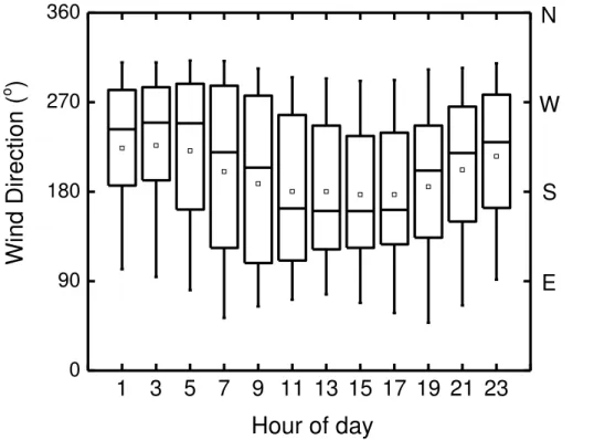
power plants, many of which lie at the Lake Michigan shoreline in the Gary-Chicago-Milwaukee urban corridor from Indiana to Wisconsin. The diurnal wind patterns (Fig. 3) at the Kenosha Harbor site also contribute to the apparent higher concentrations of ozone and SO₂ over the lake because the lake breeze wind pattern drives winds from land offshore at night (when NO2and formaldehyde losses were minimized) and from

5

the lake onshore during the day (when ozone concentrations were at a maximum). These DOAS observations align with past studies of Lake Michigan air quality in that they implicate higher O3 concentrations over Lake Michigan (Dye et al., 1995; Foley

et al., 2011; Lennartson and Schwartz, 1999, 2002). The higher SO2 concentrations

may show the influence of power plant emissions mixing over longer distances and

10

timescales over the lake. Foley et al. described (2011) sampling high NO_x plumes over Lake Michigan that appeared to remain aloft. They suggested that these plumes originated from power plants in the region, which would also be a source of SO2. The

shoreline observations presented here do not constrain the extent to which ozone was higher over the lake, nor the distribution of ozone across the lake, but only show that air

15

with enhanced ozone was observed during afternoon hours when the air moved inland during the lake breeze. At the intersection between the o_ffshore environment and the onshore environment, titration of O3occurs via emissions from local NOxsources, and

therefore the additional offshore processing cannot be distinguished from chemistry at the shoreline with this DOAS measurement alone.

20

3.2 Comparison between shoreline DOAS and ferry observations

Kenosha shoreline DOAS observations of O3 were compared with the Lake Express

ferry O3 observations in order to understand the regional distribution of ozone. The

two measurements were compared by averaging the ferry measurements to 30 min intervals at the timescale of the Kenosha harbor DOAS measurements. The diff

er-25

ences in 30 min averaged data from 2009, as measured as O3 (Lake Express Ferry)−

(11)

ACPD

14, 23201–23236, 2014

P. A. Cleary et al.

Title Page

Tables Figures

◭ ◮

Back Close

Full Screen / Esc

Discussion

P

a

per

|

Discus

sion

P

a

per

|

Discussion

P

a

per

|

Discussion

P

a

per

|

had a range of 39 to−9 ppb, a median of 4.2 ppb, mean of 5.0 ppb, standard deviation

7.6 ppb.

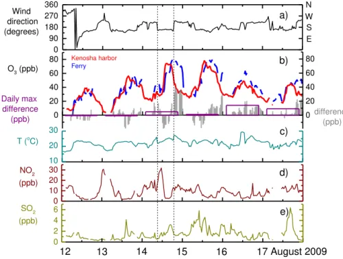
In order to demonstrate the agreement between ozone measurements of both plat-forms, Fig. 4 shows the wind direction, O₃ measurements, the difference in ozone measurements, temperature, NO2, SO2and formaldehyde for 12 to 18 August 2009. In

5

the example of 12 August 2009 in Fig. 4, the ozone mixing ratios for both instruments appear quite similar. Note that the discontinuities in ferry data represent times when the ferry was in port, and each of the segments between the data gaps represents an en-tire transect of Lake Michigan. In some cases, such as 12 August, there was very little variation in the difference between ferry and shoreline O₃with respect to the location of

10

the ferry. For 13 August, the maximum ozone as measured at the shoreline (∼50 ppb)

was observed by the ferry upon return to the western side of Lake Michigan and again when it left with roughly a 15 ppb difference between the eastern and western sides of Lake Michigan in the afternoon hours. NO₂ measurements in Fig. 4d peaked at night as high as 30 ppb and at were at a minimum during the day, particularly after noon.

15

The concentrations of NO2for this period do not correlate with SO2concentrations and

so can be considered to be from di_fferent emissions sources, such as urban non-point source NOxand power-plant or industrial sources of SO2.

Evidence of lake breeze shifts in the data was most clearly shown on 14 August (indicated by dotted lines in Fig. 4). The wind direction shifted abruptly from

south-20

west (offshore flow) until about 10:00 CDT, when it shifted to southeast (onshore flow). The temperature change between these two air masses is evident in Fig. 4c, where the ambient temperature dropped 3◦_{C as the wind direction shifted. The NO}

2

con-centration increased to 30 ppb after the wind shift, which may be evidence of recent land-based NO2 emissions from the northern Chicago area flowing offshore during

25

rush-hour and then returning onto land after the wind shift. Following the rapid NO₂ decrease, O3 increased as measured at the shoreline and also as measured on the

(12)

ACPD

14, 23201–23236, 2014

P. A. Cleary et al.

Title Page

Tables Figures

◭ ◮

Back Close

Full Screen / Esc

Discussion

P

a

per

|

Discus

sion

P

a

per

|

Discussion

P

a

per

|

Discussion

P

a

per

|

of ozone remained high. The NO₂ concentrations also rebounded to 12 ppb. In this case, the maximum SO2observations arrived at the Kenosha harbor site from offshore

later in the afternoon before the wind shifted. A Hysplit back trajectory model was cal-culated for the morning of 14 August for synoptic winds at 250 m a.g.l. and indicated an air mass arriving from the northeastern suburbs of Chicago, Illinois which would

5

intercept the rush-hour traffic emissions. Thus, the low O3mid-morning was a result of

near-source and early-day NO_xtitration. On 13–15 August NO₂increased following the wind shift between south-westerly and south-easterly wind flows. Hysplit back trajec-tories were generated for each of these days, which showed air mases from Chicago transported northward along the shoreline at the same time of day. Emissions were

10

likely brought back on land from lake breezes which could not be resolved from back trajectories.

Differences between ferry O3 and shoreline DOAS O3 mixing ratios were evaluated

with respect to temperature (Fig. 5), location of the ferry (Fig. 6) and wind direction (Fig. 7). Each figure shows the data for all times of the day, and for distinct time windows

15

(06:00–12:00 CDT, 12:00–18:00 CDT, 18:00–02:00 CDT) in box plots which represent mean (line), median (_{), 25–75 % (box), and 10–90 % (whiskers) for the 30 min average}

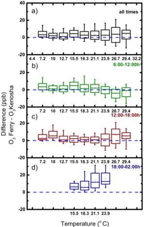
difference between O3 (Lake Express) and O3 (Kenosha Harbor). Figure 5 shows differences

between ozone observations from the ferry and shoreline with respect to temperature. There was no observed trend in di_fference in ozone vs. temperature for all data, a

mi-20

nor trend for morning times (06:00–12:00 CDT, Fig. 5b) where the difference changed from a positive difference to a more negative difference with increasing temperature above 15.5◦_{C, and an opposite trend toward higher ozone over the lake in the} after-noon (12:00–18:00 CDT) and for temperatures above 26◦C. Ozone differences after 18:00 CDT show consistently higher ozone concentrations over the lake for all

temper-25

(13)

ACPD

14, 23201–23236, 2014

P. A. Cleary et al.

Title Page

Tables Figures

◭ ◮

Back Close

Full Screen / Esc

Discussion

P

a

per

|

Discus

sion

P

a

per

|

Discussion

P

a

per

|

Discussion

P

a

per

|

from inland in the late evening, they could have been chemically different from those found far offshore. The only time when shoreline DOAS ozone observations tended to be higher than those from the ferry was at 06:00–12:00 CDT for temperatures above 26.7◦C. This may be due to days when temperatures were high in the morning, thus stagnating the air and limiting the influence of lake/land breeze on horizontal movement

5

of airmasses. Differences in offshore and shoreline observations of ozone with respect to temperature were largest later in the day and at higher temperatures when ozone was typically at a maximum.

Investigations into the ozone differences between shoreline and ferry observations with respect to ferry location were conducted as a test of the east-west gradient over

10

Lake Michigan. Figure 6 depicts the di_fference of O_{3 (Lake Express)}−O3 (Kenosha Harbor)with

respect to ferry distance from Milwaukee. For all data the mean and median difference was positive (i.e., greater as measured over water from the ferry). The median diff er-ences were not significantly positive or negative for the morning, slightly positive for the early afternoon time window, and consistently positive for the late afternoon/evening. In

15

the case of the late evening time window, the mean, median and extremes (25–75 %) of the data all lie above 0, which is a strong suggestion that at these times the ozone concentrations over the lake are consistently higher than at the shoreline. However, there does not appear to be a significant variation with respect to longitude, meaning that evaluated as a whole, the land-lake di_fferences in ozone did not depend on the

20

ferry’s distance from the shoreline. This demonstrates a widely regional distribution of ozone once over the lake.

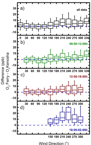
In order to distinguish between meteorological e_ffects at the shoreline, the di_ff er-ences in ozone observations from the ferry and shoreline DOAS ozone concentrations with respect to wind direction at Kenosha Harbor were evaluated. All data (Fig. 7a)

25

(14)

ACPD

14, 23201–23236, 2014

P. A. Cleary et al.

Title Page

Tables Figures

◭ ◮

Back Close

Full Screen / Esc

Discussion

P

a

per

|

Discus

sion

P

a

per

|

Discussion

P

a

per

|

Discussion

P

a

per

|

evening/night, the largest differences were observed after 18:00 CDT if winds were ar-riving from 180–360◦. This picture is consistent with land breezes developing in the evening and producing surface winds which draw from land and move over the lake. The sampled air masses at the shoreline, thus, were of different origin (or sampled air masses over the lake were isolated from land-based air masses). The number of data

5

points (n <15) were acquired when the wind blew from 30–160◦from 18:00–02:00 CDT

were insufficient for analysis. For the morning and early afternoon times, the trend with respect to wind direction was not large.

Figures 5–7 indicate that the differences between ferry and shoreline ozone obser-vations were largest in the time window after 18:00 CDT and into the night. The diff

er-10

ence between the ferry and shoreline trend with the wind direction for all times of the day with the mean difference for wind directions from 0–180◦ at 0.2 ppb and for wind directions from 180–360◦ at 6.3 ppb. This trend in the dependence of the observed ozone di_fference with respect to wind direction is magnified after noon. One possible key driver of differences between observed offshore and shoreline ozone could be the

15

differences in NOxemissions from each wind direction. The trends with respect to

tem-perature are small in comparison to the trends with respect to wind direction and may be a subtle indicator of the strength of lake breeze effects. Both temperature and lo-cation may demonstrate some differences in photochemistry, where some aspects of photochemical ozone production are enhanced with temperature (water vapor content,

20

VOC emissions), the distance from emissions sources (where titration of O3can occur)

could be represented by the distance from the western Lake Michigan shoreline, and lower losses of O₃to water surfaces compared to terrestrial surfaces (Levy et al., 2010). One complicating factor is that the ferry intercepted air near the surface, whereas ur-ban plumes might reside aloft over an inversion above the lake (Foley et al., 2011;

25

(15)

ACPD

14, 23201–23236, 2014

P. A. Cleary et al.

Title Page

Tables Figures

◭ ◮

Back Close

Full Screen / Esc

Discussion

P

a

per

|

Discus

sion

P

a

per

|

Discussion

P

a

per

|

Discussion

P

a

per

|

Levy et al. (2010) where oscillations in inland ozone were observed at times associated with lake-breeze front movement. The extent to which inversion occurs over the lake at night and ozone precursors and ozone concentrations remain high aloft, as suggested by Dye et al. and Foley et al. (Foley et al., 2011; Dye et al., 1995) cannot be evaluated by our measurements at the surface.

5

3.3 Comparison of ferry ozone with National Air Quality Forecast Model

The National Air Quality Forecast Model output predicts ozone concentrations at sur-face locations across the US. These forecasts produce a distinct ozone maximum over the water surfaces of the Great Lakes and, in particular, southern Lake Michigan. Im-ages of the hourly forecasts in the Upper Midwestern region surrounding Lake Michigan

10

(Fig. 8) were saved for the monitoring season of 2009 from 18 June–3 November 2009 for the hours of 08:00–22:00 CDT. To process the images for comparison with observa-tions, they were digitized, converted to a common time stamp and georeferenced. The comparison between the ozone forecast and the observations along the ferry transect were then computed. The bias of the model, defined as:

15

bias₌p_i₋o_i (1)

wherep_i is the model-predicted O₃ concentration ando_i is the observed O₃

concen-tration on the ferry, was determined by hourly-averaged ferry observations geospatially matched to the time stamp (using CDT) of the model image outputs. The geospatial

20

location was established at the average ferry location for the 1 h average, excluding any time spent in port. The mean ferry trip time was 2.25 h, so this method of analy-sis resulted in approximately 2 model comparisons per ferry trip with a minimum of 30 1 min points per comparison when port data was omitted. For all 1 h average data, the bias is consistently high, with a 12 ppb mean over-prediction of ozone. The magnitude

25

(16)

ACPD

14, 23201–23236, 2014

P. A. Cleary et al.

Title Page

Tables Figures

◭ ◮

Back Close

Full Screen / Esc

Discussion

P

a

per

|

Discus

sion

P

a

per

|

Discussion

P

a

per

|

Discussion

P

a

per

|

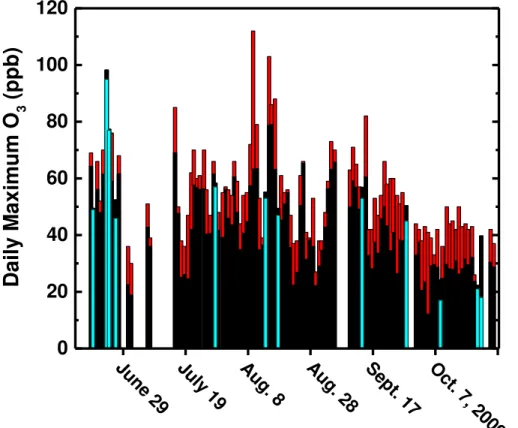
O₃ on the ferry (black) was compared to the 1 h average forecast ozone which show the amount of over-prediction added to the observed value (red) or up to the under-predicted value (blue), at the particular location of the observed ferry maximum. The reported maximum ozone bias was only as observed by the ferry and does not neces-sarily capture the global maximum ozone over Lake Michigan. The mean bias for the

5

daily maximum O3(as observed by the ferry) is 10 ppb, which is lower than the mean

bias for all daytime 1 h data of 12 ppb.

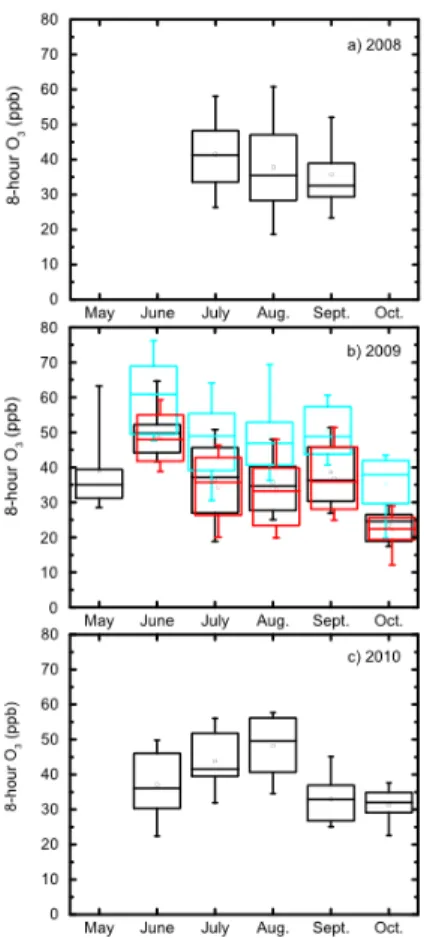
The 8 h average ozone was computed for the ferry observations, Kenosha Harbor observations and NAQFM forecast concentrations in 2008, 2009 and 2010 (Fig. 10). The 8 h average for the ferry observations was for periods when the ferry was most

10

likely to be in operation (10:00–18:00 CDT), and thus is a restricted representation of the ozone over the lake with respect to typical methods for evaluating federal air quality standards for stationary, continuous monitoring. The 8 h ozone mean bias is 12 ppb for the sampling period in 2009. Mean bias of the NAQFM for 8 h average ozone is 11 ppb for June, 12 ppb for July, 13 ppb for August, 12 ppb for September and 11 ppb for

15

October. For all 3 years, there were no observed exceedences of the federal standard (8 h O₃ >75 ppb). In the case of 2009, the ferry observations were _∼5 ppb higher

than the shoreline Kenosha harbor observations except in June. The NAQFM forecasts predicted 2 exceedences of 8 h O3 in June 2009, but no data from the shoreline or

ferry exceeded the standard for that month. NAQFM model output and Kenosha harbor

20

measurements were not available for May 2009.

Others have also found the NAQFM to predict ozone concentrations that were bi-ased high (Eder et al., 2009; Tang et al., 2009; Zhang et al., 2012a, b; Wilczak et al., 2006). Simon et al. (2012) completed an exhaustive comparison of photochemical per-formance statistics reported from 2006–2012, whereby national median in mean bias

25

(17)

ACPD

14, 23201–23236, 2014

P. A. Cleary et al.

Title Page

Tables Figures

◭ ◮

Back Close

Full Screen / Esc

Discussion

P

a

per

|

Discus

sion

P

a

per

|

Discussion

P

a

per

|

Discussion

P

a

per

|

between the median and 75th percentile for the 22 studies of 1 h maximum ozone and higher than 75 % of 60 studies of 8 h maximum ozone. The work presented here represents the first study of model bias over the water of Lake Michigan.

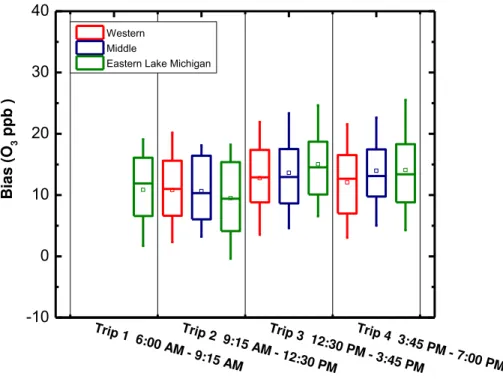
The 1 h model O₃ bias was evaluated for trends with respect to time of day (as organized by trip of the day) and ferry location: Western Lake Michigan (ferry longitude

5

>87.3◦W), Middle Lake Michigan (ferry longitude between 87.3◦W and 86.7◦W) and

Eastern Lake Michigan (ferry longitude<86.7◦W) (Fig. 11). In the later trips of the day

(3 and 4) the 1 h O3bias tends to increase from west to east for most statistical markers

of the data (mean, median, 75 % and 90 %), whereas that trend is slightly reversed for Trip 2 of the day. While these trends in the bias were small (∼2 ppb) in comparison

10

to the mean bias (12 ppb), the spatial trends in the bias provide clues regarding the mechanisms that result in over-prediction in the model. In particular, the ferry transect was oriented east–west and the emission sources of ozone precursors predominantly lie at the western shoreline of Lake Michigan. Therefore, the observed trend of a higher bias at the eastern side of Lake Michigan in the afternoon may indicate insufficient

15

ozone loss mechanisms in the forecast model, production of ozone extending farther away from emissions sources, or boundary layer or other meteorological confinement of the air mass properties that are not symmetric across the lake.

The model bias was also evaluated with respect to month for the 3 regions (Fig. 12). The only two months which showed most significant di_fferences in model bias with

20

respect to ferry position were June and October. In June, the bias in the middle of Lake Michigan was higher than the western or eastern sides of Lake Michigan (which is shown in the 90th percentile, 75th percentile, median, mean and 25th percentile, 10th percentile). A similar trend was shown in July (as shown in 75th percentile, me-dian, mean, 25th percentile and 10th percentile) and August (as observed in the 90th

25

(18)

ACPD

14, 23201–23236, 2014

P. A. Cleary et al.

Title Page

Tables Figures

◭ ◮

Back Close

Full Screen / Esc

Discussion

P

a

per

|

Discus

sion

P

a

per

|

Discussion

P

a

per

|

Discussion

P

a

per

|

meteorology between June (lake colder than overland air) and October (lake warmer than overland air). Also, O3production is limited in October and 8 h average

concentra-tions were around 30 ppb, so these differences could be attributed to the difference in chemistry (limited production or enhanced loss mechanisms). The extent to which the parameterization of mesoscale meteorological effects or other model parameters like

5

emissions and chemistry influence the O3model forecast cannot be extracted from this

analysis. Without specific tests of the structure and parameterization of the NAQFM, these trends cannot be further dissected.

The time of day and position of the forecasted and observed daily maximum ozone concentrations are given in Figs. 13 and 14. The data are presented as histograms that

10

represent the number of days where the maximum ozone was located within a particu-lar range of latitudes or within a given hour. The hour that most frequently corresponded to the maximum ozone concentration was 16:00 CDT for both the NAQFM and the ferry observations. Fewer total observations around 15:00 CDT may account for the small number of maximum ozone observations at that time because the ferry was typically in

15

port at that time. The location of the daily maximum ozone from the ferry varies from the distribution given by the NAQFM (Fig. 14). The NAQFM predicts the highest fre-quency of daily maximum O3 will most frequently be just offshore on the eastern side

of Lake Michigan, whereas this was not observed by the ferry. However, the ferry may not have captured the time of maximum O₃at the eastern side of Lake Michigan, as its

20

typical trip began in Muskegon at 16:00 CDT.

4 Conclusions

Observations of shoreline O₃and ferry O₃in comparison to forecast O₃by the NAQFM show more agreement between shoreline and the ferry measurements than ozone fore-casts over the lake and ferry measurements. Shoreline Lake Michigan measurements

25

(19)

ACPD

14, 23201–23236, 2014

P. A. Cleary et al.

Title Page

Tables Figures

◭ ◮

Back Close

Full Screen / Esc

Discussion

P

a

per

|

Discus

sion

P

a

per

|

Discussion

P

a

per

|

Discussion

P

a

per

|

shoreline DOAS O₃ observations indicated that diurnal changes in ozone concentra-tion were larger than spatial gradients across Lake Michigan, and ozone tended to be higher over Lake Michigan, particularly in the evening. Mesoscale meteorological processes involving differential heating between the lake and land surfaces produced diurnal cycles of air mass flow between shoreline environments and offshore, which

5

complicated the understanding of offshore ozone dynamics. The ferry-based 1 h O3

observations were on average 12 ppb below NAQFM predictions. The NAQFM con-sistently predicted higher ozone than observed over water, with biases higher than a majority of previously published model performance statistics (Simon et al., 2012). The bias of the NAQFM showed some trends in increasing to the eastern side of Lake

10

Michigan when evaluated with respect to ferry trip, and a complicated bias of higher over-prediction mid-lake in the spring and summer, switching to a lower over-prediction mid-lake in fall. Ferry ozone observations captured 0 exceedances in 8 h ozone in com-parison to 2 predicted by NAQFM. Further analyses are required to determine whether NAQFM predictions might be improved by adjusting model parameters related to

emis-15

sion sources, mesoscale meteorology, or atmospheric chemistry.

Acknowledgements. The authors would like to thank Kaya Sims and Renee Hanson for their assistance in this experiment, the Lake Express Ferry, University of Wisconsin-Eau Claire Office of Sponsored Programs Faculty and Student Collaboration Grant, Great Lakes Water Institute, Kenosha Water Utility and the Great Lakes Observing System for their cooperation and support

20

of this project. The authors would like to thank Bruce E. Brown for assistance with collection and calibration of ozone data from the Lake Express ferry, and Kenneth Aikin for archiving of NAQFM images. Thomas Langel acknowledges the NOAA Hollings Scholar Program for fellow-ship support during 2010. SSB acknowledges support from NOAA’s Atmospheric Chemistry, Carbon Cycle and Climate Program.

(20)

ACPD

14, 23201–23236, 2014

P. A. Cleary et al.

Title Page

Tables Figures

◭ ◮

Back Close

Full Screen / Esc

Discussion

P

a

per

|

Discus

sion

P

a

per

|

Discussion

P

a

per

|

Discussion

P

a

per

|

References

Carpenter, L. J., Sturges, W. T., Penkett, S. A., Liss, P. S., Alicke, B., Hebestreit, K., and Platt, U.: Short-lived alkyl iodides and bromides at Mace Head, Ireland: links to biogenic sources and halogen oxide production, J. Geophys. Res.-Atmos., 104, 1679–1689, 1999.

Dye, T. S., Roberts, P. T., and Korc, M. E.: Observations of transport processes for ozone and

5

ozone precursors during the 1991 Lake Michigan Ozone Study, J. Appl. Meteorol., 34, 1877– 1889, 1995.

Eder, B., Kang, D. W., Mathur, R., Pleim, J., Yu, S. C., Otte, T., and Pouliot, G.: A performance evaluation of the National Air Quality Forecast Capability for the summer of 2007, Atmos. Environ., 43, 2312–2320, 2009.

10

Fast, J. D. and Heilman, W. E.: The effect of lake temperatures and emissions on ozone expo-sure in the western Great Lakes region, J. Appl. Meteorol., 42, 1197–1217, 2003.

Fast, J. D. and Heilman, W. E.: Simulated sensitivity of seasonal ozone exposure in the Great Lakes region to changes in anthropogenic emissions in the presence of interannual variabil-ity, Atmos. Environ., 39, 5291–5306, 2005.

15

Foley, T., Betterton, E. A., Jacko, P. E. R., and Hillery, J.: Lake Michigan air quality: the 1994– 2003 LADCO Aircraft Project (LAP), Atmos. Environ., 45, 3192–3202, 2011.

Hanna, S. R. and Chang, J. C.: Relations between meteorology and ozone in the Lake Michigan region, J. Appl. Meteorol., 34, 670–678, 1995.

Harris, L. and Kotamarthi, V. R.: The characteristics of the Chicago Lake breeze and its effects

20

on trace particle transport: results from an episodic event simulation, J. Appl. Meteorol., 44, 1637–1654, 2005.

Keen, C. S. and Lyons, W. A.: Lake/Land Breeze circulations on the western shore of Lake Michigan, J. Appl. Meteorol., 17, 1843–1855, 1978.

Lennartson, G. J. and Schwartz, M. D.: A synoptic climatology of surface-level ozone in Eastern

25

Wisconsin, USA, Clim. Res., 13, 207–220, 1999.

Lennartson, G. J. and Schwartz, M. D.: The lake breeze-ground-level ozone connection in eastern Wisconsin: a climatological perspective, Int. J. Climatol., 22, 1347–1364, 2002. Levy, I., Makar, P. A., Sills, D., Zhang, J., Hayden, K. L., Mihele, C., Narayan, J., Moran, M. D.,

Sjostedt, S., and Brook, J.: Unraveling the complex local-scale flows influencing ozone

pat-30

(21)

ACPD

14, 23201–23236, 2014

P. A. Cleary et al.

Title Page

Tables Figures

◭ ◮

Back Close

Full Screen / Esc

Discussion

P

a

per

|

Discus

sion

P

a

per

|

Discussion

P

a

per

|

Discussion

P

a

per

|

Lyons, W. A. and Cole, H. S.: Photochemical oxidant transport – mesoscale lake breeze and synoptic-scale aspects, J. Appl. Meteorol., 15, 733–743, 1976.

Lyons, W. A. and Olsson, L. E.: Detailed mesometeorological studies of air pollution dispersion in Chicago lake breeze, Mon. Weather Rev., 101, 387–403, 1973.

Martin, J. C. G., Mahajan, A. S., Hay, T. D., Prados-Roman, C., Ordonez, C., MacDonald, S. M.,

5

Plane, J. M. C., Sorribas, M., Gil, M., Mora, J. F. P., Reyes, M. V. A., Oram, D. E., Leed-ham, E., and Saiz-Lopez, A.: Iodine chemistry in the eastern Pacific marine boundary layer, J. Geophys. Res.-Atmos., 118, 887–904, 2013.

Martinez, M., Perner, D., Hackenthal, E. M., Kulzer, S., and Schutz, L.: NO₃at Helgoland dur-ing the NORDEX campaign in October 1996, J. Geophys. Res.-Atmos., 105, 22685–22695,

10

2000.

Rivera, C., Mellqvist, J., Samuelsson, J., Lefer, B., Alvarez, S., and Patel, M. R.: Quantifi-cation of NO₂ and SO₂ emissions from the Houston Ship Channel and Texas City indus-trial areas during the 2006 Texas Air Quality Study, J. Geophys. Res.-Atmos., 115, D08301 doi:10.1029/2009JD012675, 2010.

15

Seitz, K., Buxmann, J., Pöhler, D., Sommer, T., Tschritter, J., Neary, T., O’Dowd, C., and Platt, U.: The spatial distribution of the reactive iodine species IO from simultaneous active and passive DOAS observations, Atmos. Chem. Phys., 10, 2117–2128, doi:10.5194/acp-10-2117-2010, 2010.

Simon, H., Baker, K. R., and Phillips, S.: Compilation and interpretation of photochemical model

20

performance statistics published between 2006 and 2012, Atmos. Environ., 61, 124–139, 2012.

Takashima, H., Irie, H., Kanaya, Y., and Akimoto, H.: Enhanced NO₂at Okinawa Island, Japan caused by rapid air-mass transport from China as observed by MAX-DOAS, Atmos. Environ., 45, 2593–2597, 2011.

25

Tang, Y. H., Lee, P., Tsidulko, M., Huang, H. C., McQueen, J. T., DiMego, G. J., Emmons, L. K., Pierce, R. B., Thompson, A. M., Lin, H. M., Kang, D. W., Tong, D., Yu, S. C., Mathur, R., Pleim, J. E., Otte, T. L., Pouliot, G., Young, J. O., Schere, K. L., Davidson, P. M., and Stajner, I.: The impact of chemical lateral boundary conditions on CMAQ predictions of tropospheric ozone over the continental United States, Environ. Fluid Mech., 9, 43–58, 2009.

30

(22)

ACPD

14, 23201–23236, 2014

P. A. Cleary et al.

Title Page

Tables Figures

◭ ◮

Back Close

Full Screen / Esc

Discussion

P

a

per

|

Discus

sion

P

a

per

|

Discussion

P

a

per

|

Discussion

P

a

per

|

eastern Mediterranean troposphere during the MINOS campaign, Atmos. Chem. Phys., 4, 169–182, doi:10.5194/acp-4-169-2004, 2004.

White, M. L., Russo, R. S., Zhou, Y., Mao, H., Varner, R. K., Ambrose, J., Veres, P., Wingen-ter, O. W., Haase, K., Stutz, J., Talbot, R., and Sive, B. C.: Volatile organic compounds in northern New England marine and continental environments during the ICARTT 2004

cam-5

paign, J. Geophys. Res.-Atmos., 113, D08S90, doi:10.1029/2007JD009161, 2008.

Wilczak, J., McKeen, S., Djalalova, I., Grell, G., Peckham, S., Gong, W., Bouchet, V., Moffet, R., McHenry, J., McQueen, J., Lee, P., Tang, Y., and Carmichael, G. R.: Bias-corrected ensemble and probabilistic forecasts of surface ozone over eastern North America during the summer of 2004, J. Geophys. Res.-Atmos., 111, D23S28, doi:10.1029/2006JD007598, 2006.

10

Zhang, Y., Bocquet, M., Mallet, V., Seigneur, C., and Baklanov, A.: Real-time air quality forecast-ing, Part I: History, techniques, and current status, Atmos. Environ., 60, 632–655, 2012a. Zhang, Y., Bocquet, M., Mallet, V., Seigneur, C., and Baklanov, A.: Real-time air quality

fore-casting, Part II: State of the science, current research needs, and future prospects, Atmos. Environ., 60, 656–676, 2012b.

(23)

ACPD

14, 23201–23236, 2014

P. A. Cleary et al.

Title Page

Tables Figures

◭ ◮

Back Close

Full Screen / Esc

Discussion

P

a

per

|

Discus

sion

P

a

per

|

Discussion

P

a

per

|

Discussion

P

a

per

|

(24)

ACPD

14, 23201–23236, 2014

P. A. Cleary et al.

Title Page

Tables Figures

◭ ◮

Back Close

Full Screen / Esc

Discussion

P

a

per

|

Discus

sion

P

a

per

|

Discussion

P

a

per

|

Discussion

P

a

per

|

Figure 2.Wind rose depictions of median concentration of (a) O₃ (b) NO₂ (c) SO₂ and (d)

formaldehyde with respect to wind direction as measured by DOAS at Kenosha harbor from April–November 2009. Medians are not reported for wind directions where few measure-ments (n <75 for 30 min averaged data points) were above the detection limit (d.l.=1.5 ppb

(25)

ACPD

14, 23201–23236, 2014

P. A. Cleary et al.

Title Page

Tables Figures

◭ ◮

Back Close

Full Screen / Esc

Discussion

P

a

per

|

Discus

sion

P

a

per

|

Discussion

P

a

per

|

Discussion

P

a

per

|

November of 2009. Box plots show mean (□)

1

3

5

7 9 11 13 15 17 19 21 23

0

90

180

270

360 E

S

W

Hour of day

Win

d Di

re

ct

io

n (

o

)

N

(26)

ACPD

14, 23201–23236, 2014

P. A. Cleary et al.

Title Page Abstract Introduction Conclusions References Tables Figures ◭ ◮ ◭ ◮ Back Close

Full Screen / Esc

Printer-friendly Version Interactive Discussion Discussion P a per | Discus sion P a per | Discussion P a per | Discussion P a per | 0 20 40 60 80 O₃ (ppb)

Kenosha harbor Ferry 0 20 40 60 80 Daily max difference

(ppb) difference_(ppb)

0 90 180 270 360 e) d) c) b) Wind direction (degrees) a) N W S E 0 2 4 6 17 16 15 14 13 SO₂ (ppb) August 2009 12 0 10 20 30 NO₂ (ppb) 10 20 30 T (oC)

(27)

ACPD

14, 23201–23236, 2014

P. A. Cleary et al.

Title Page

Tables Figures

◭ ◮

Back Close

Full Screen / Esc

Discussion

P

a

per

|

Discus

sion

P

a

per

|

Discussion

P

a

per

|

Discussion

P

a

per

|

02:00h). Box plots show mean (□),

Figure 5.Difference in O₃ observations between platforms with respect to temperature (◦_C) measured at the shoreline for(a)all times,(b)morning (06:00–12:00 CDT),(c)early afternoon (12:00–16:00 CDT) and(d)late afternoon/evening (16:00–02:00h). Box plots show mean (_),

(28)

ACPD

14, 23201–23236, 2014

P. A. Cleary et al.

Title Page

Tables Figures

◭ ◮

Back Close

Full Screen / Esc

Discussion

P

a

per

|

Discus

sion

P

a

per

|

Discussion

P

a

per

|

Discussion

P

a

per

|

02:00h). Box plots show mean (□), median (centerline), 25%

(29)

ACPD

14, 23201–23236, 2014

P. A. Cleary et al.

Title Page

Tables Figures

◭ ◮

Back Close

Full Screen / Esc

Discussion

P

a

per

|

Discus

sion

P

a

per

|

Discussion

P

a

per

|

Discussion

P

a

per

|

mean (□), median (

Figure 7.Difference in O₃observations between platforms with respect to wind direction mea-sured at Kenosha harbor for(a)all times, (b)morning (06:00–12:00 CDT),(c)early afternoon (12:00–16:00 CDT) and(d)late afternoon/evening (16:00–02:00h). Box plots show mean (_),

(30)

ACPD

14, 23201–23236, 2014

P. A. Cleary et al.

Title Page

Tables Figures

◭ ◮

Back Close

Full Screen / Esc

Discussion

P

a

per

|

Discus

sion

P

a

per

|

Discussion

P

a

per

|

Discussion

P

a

per

|

(31)

ACPD

14, 23201–23236, 2014

P. A. Cleary et al.

Title Page

Tables Figures

◭ ◮

Back Close

Full Screen / Esc

Discussion

P

a

per

|

Discus

sion

P

a

per

|

Discussion

P

a

per

|

Discussion

P

a

per

|

0

20

40

60

80

100

120 Da

il

y Max

imum O

3

(ppb

)

Ju ne

29 Ju

ly 19

Aug . 8

Aug . 2

8 Sept

. 1 7

Oct . 7

, 2 00

9

(32)

ACPD

14, 23201–23236, 2014

P. A. Cleary et al.

Title Page

Tables Figures

◭ ◮

Back Close

Full Screen / Esc

Discussion

P

a

per

|

Discus

sion

P

a

per

|

Discussion

P

a

per

|

Discussion

P

a

per

|

(33)

ACPD

14, 23201–23236, 2014

P. A. Cleary et al.

Title Page

Tables Figures

◭ ◮

Back Close

Full Screen / Esc

Discussion

P

a

per

|

Discus

sion

P

a

per

|

Discussion

P

a

per

|

Discussion

P

a

per

|

Trip 1 6:0

0 AM - 9:15 A_M Trip

2 9:1 5 AM -

12:30_PM Trip

3 12:30_PM

- 3:4_{5 PM} Trip

4 3:4_{5 PM -} 7:00 PM

Bias

(

O3

ppb

)

Figure 11.Bias in NAQFM ozone forecast compared to ferry measurement spatially matched to location of the ship with respect to time of day. The bias per trip was evaluated by selecting data only when the ferry trip was occurring in the typical trip time window given. The bias was evaluated for 3 regions of Lake Michigan: western Lake Michigan, ferry longitude>87.3◦W, middle Lake Michigan, ferry longitude between 87.3◦W and 86.7◦W, and eastern Lake Michi-gan, ferry longitude<86.7◦W. Box plots show mean (_{), median (centerline), 25–75 % (box)}

(34)

ACPD

14, 23201–23236, 2014

P. A. Cleary et al.

Title Page

Tables Figures

◭ ◮

Back Close

Full Screen / Esc

Discussion

P

a

per

|

Discus

sion

P

a

per

|

Discussion

P

a

per

|

Discussion

P

a

per

|

Ju_ne Ju_ly Aug

us_t Septembe

r Oct

ob er 20

09

Bias

(O

3

p

pb

)

Figure 12. Bias in NAQFM ozone forecast compared to ferry measurement with respect to month. The bias was evaluated for 3 regions of Lake Michigan: western Lake Michigan, ferry longitude>87.3◦W, middle Lake Michigan, ferry longitude between 87.3◦W and 86.7◦W and

eastern Lake Michigan, ferry longitude<86.7◦W. Box plots show mean (), median

(35)

ACPD

14, 23201–23236, 2014

P. A. Cleary et al.

Title Page

Tables Figures

◭ ◮

Back Close

Full Screen / Esc

Discussion

P

a

per

|

Discus

sion

P

a

per

|

Discussion

P

a

per

|

Discussion

P

a

per

|

8 9 10 11 12 13 14 15 16 17 18 19 20 21 22 23

0 10 20

b)

number

hour of day

Ferry

8 9 10 11 12 13 14 15 16 17 18 19 20 21 22 23

0 10 20

a)

number

NAQFM

(36)

ACPD

14, 23201–23236, 2014

P. A. Cleary et al.

Title Page

Tables Figures

◭ ◮

Back Close

Full Screen / Esc

Discussion

P

a

per

|

Discus

sion

P

a

per

|

Discussion

P

a

per

|

Discussion

P

a

per

|

0 20 40 60 80 100 120 140 160

0 5 10 15 20

number

NAQFM a)

0 20 40 60 80 100 120 140 160

0 5 10 15 20

b)

number

distance from Milwaukee (km)

Ferry