www.atmos-chem-phys.net/10/7697/2010/ doi:10.5194/acp-10-7697-2010
© Author(s) 2010. CC Attribution 3.0 License.
Chemistry
and Physics
Options to accelerate ozone recovery: ozone and climate benefits
J. S. Daniel1, E. L. Fleming2,3, R. W. Portmann1, G. J. M. Velders4, C. H. Jackman2, and A. R. Ravishankara1 1National Oceanic and Atmospheric Administration, Earth System Research Laboratory, Chemical Sciences Division,
Boulder, CO 80305, USA
2NASA Goddard Space Flight Center, Greenbelt, Maryland, 20771, USA 3Science Systems and Applications, Inc., Lanham, MD 20706, USA
4Netherlands Environmental Assessment Agency, 3720 AH Bilthoven, The Netherlands
Received: 23 March 2010 – Published in Atmos. Chem. Phys. Discuss.: 23 April 2010 Revised: 22 June 2010 – Accepted: 11 July 2010 – Published: 18 August 2010
Abstract. Hypothetical reductions in future emissions of ozone-depleting substances (ODSs) and N2O are evaluated
in terms of effects on equivalent effective stratospheric chlo-rine (EESC), globally-averaged total column ozone, and ra-diative forcing through 2100. Due to the established success of the Montreal Protocol, these actions can have only a frac-tion of the impact on ozone deplefrac-tion that regulafrac-tions already in force have had. If all anthropogenic ODS and N2O
emis-sions were halted beginning in 2011, ozone is calculated to be higher by about 1–2% during the period 2030–2100 com-pared to a case of no additional restrictions. Direct radia-tive forcing by 2100 would be about 0.23 W/m2lower from the elimination of anthropogenic N2O emissions and about
0.005 W/m2lower from the destruction of the chlorofluoro-carbon (CFC) bank. Due to the potential impact of N2O on
future ozone levels, we provide an approach to incorporate it into the EESC formulation, which is used extensively in ozone depletion analyses. The ability of EESC to describe total ozone changes arising from additional ODS and N2O
controls is also quantified.
1 Introduction
The Montreal Protocol on Substances that Deplete the Ozone Layer and its amendments and adjustments have been suc-cessful in halting the decline in global ozone (WMO, 2007); these actions have also reduced climate forcing from
ozone-Correspondence to:J. S. Daniel ([email protected])
depleting substances (ODS) over the last 2 decades (Velders et al., 2007), and have thus presumably reduced the rate of climate change over this period compared to what would have otherwise occurred. The production and consumption (defined by the Montreal Protocol as production plus imports minus exports) of many of the most important chlorine- and bromine-containing ODSs are already phased out. Most of the others are controlled, with schedules in place to phase out their production and consumption in the next few decades.
However, the Protocol does not limit some types of ODS production and consumption and does not directly regulate ODS emissions at all. Several activities involving ODSs are thus expected to continue to lead to atmospheric emis-sions. Restricting these sources represents an opportunity to accelerate ozone recovery. For example, because the Mon-treal Protocol does not directly regulate emissions, it does not limit the release of ODSs already produced and cur-rently residing in existing equipment or applications, such as firefighting equipment, air conditioners, refrigerators, and foams. Production of hydrochlorofluorocarbons (HCFCs) and CH3Br also continues. Production of HCFCs is to be
nearly phased out globally by 2030 with stepwise reductions in place in the intervening time under the current Protocol. CH3Br use for quarantine and preshipment purposes is
un-restricted and critical use exemptions have been granted ev-ery year since 2005 (http://ozone.unep.org/Data Reporting/ Data Access/). Production of CCl4for non-feedstock use has
unregulated CCl4 sources could explain why global
emis-sions inferred from the CCl4global lifetime and atmospheric
mixing ratio observations have been higher than what has been suggested by reported production (WMO, 2007). What-ever the reason for this discrepancy, our inability to balance the CCl4budget with current understanding of sources and
sinks suggests that future trends are also uncertain and that emissions may continue.
Recently, it has been suggested that N2O could be
consid-ered an ODS (Ravishankara et al., 2009). While it has been known for over 4 decades that N2O leads to stratospheric
NOxproduction and subsequent ozone destruction (Crutzen,
1970), N2O has not been regulated by the Montreal
Proto-col. Ravishankara et al. (2009) quantified the global ozone depletion potential (ODP) of N2O and compared the
ODP-weighted emissions of N2O with those of regulated ODSs.
Such a comparison demonstrates that N2O is an important
gas when considering ozone depletion. N2O is also a
rec-ognized greenhouse gas that was included in the basket of gases regulated under the Kyoto Protocol. Nevertheless, pro-jections suggest that N2O emissions will remain significant
through 2100 even under strongly mitigated climate stabi-lization scenarios (Clarke et al., 2007). While there has been widespread consensus that N2O is a substance that depletes
ozone, some interpret that assigning a label of “ODS” to a compound implies a recommendation for regulation by the Montreal Protocol. Because such a recommendation cannot be justified by science alone, and because Ravishankara et al. (2009) did not make such a policy statement, we will not associate the label of ODS with N2O in the present study.
CH4(Randeniya et al., 2002) and CO2(Rosenfield et al.,
2002) are also known to substantially affect ozone levels. Although increases in CH4and CO2 are thought to lead to
reduced ozone in certain regions of the stratosphere, cal-culations show that they lead to increases in total column ozone when globally averaged. Indeed, some calculations (Portmann and Solomon, 2007) suggest that future changes in these greenhouse gases over this century may lead to in-creases in globally averaged ozone levels that are large com-pared with the historical depletion experienced due to the ODSs. Owing to their climate impact, increasing CH4 and
CO2to increase stratospheric ozone is unlikely to be a viable
policy option for reducing ozone depletion. Because of this, we do not consider such an option in the rest of this analysis. However, it should be noted that the results presented here must be considered against a backdrop of changing CO2and
CH4 levels, which will have significant global and regional
impacts on ozone.
Equivalent effective stratospheric chlorine (EESC) (Daniel et al., 1995; Newman et al., 2007) has been the tool fre-quently used to quantify the relative effectiveness of vari-ous policy options for reducing ozone depletion (e.g., WMO, 1991, 1995, 1999, 2003, 2007). It has been assumed, but not explicitly quantified, that the integrated EESC decreases from some policy action are strongly related to the integrated
ozone increases over the same time period. The EESC ap-proach has been used partly because of the significant com-puter resources required to evaluate all available options di-rectly using ozone calculated from 2-D or 3-D models. As computer speeds have increased, it has become feasible to perform these calculations with 2-D models.
Here, we consider several of the most important sources of future emissions that lead to ozone depletion and how additional controls could further limit this depletion and re-duce radiative forcing. Emissions projections that incorpo-rate reductions in these sources, along with the scenarios to which these are compared, are described in Sect. 2. Also in Sect. 2, we describe the models used to calculate ozone, and we present an approach to incorporate N2O into the global
EESC formalism. In Sect. 3, the impacts of the various op-tions for reducing future ODS and N2O emissions are
cal-culated in terms of EESC, total column ozone, and radiative forcing. The ozone results are also used to quantify the ex-tent to which the current EESC formulation serves as a suit-able metric for approximating the impacts of ODS and N2O
changes on integrated ozone changes. Conclusions are pre-sented in Sect. 4.
2 Analysis
2.1 Scenarios and hypothetical test cases
Two reference scenarios are used to evaluate the various emission reduction cases. One, which we will refer to as the “background” includes no anthropogenic ODS or N2O
emissions in the past or future; it does include observed CO2
and CH4 abundances through the present with future
mix-ing ratios prescribed by the Intergovernmental Panel on Cli-mate Change (IPCC) SRES A1B scenario (Nakicenovic et al., 2000). The background scenario also does not include the observed increase from 480 to 550 parts per trillion by volume (pptv) in CH3Cl during the 20th century (WMO,
2007). This increase may be due to natural processes, but plays a very minor role in the analysis. The second, “base-line”, scenario includes the same CO2and CH4evolution as
in the background scenario but also includes anthropogenic ODS and N2O emissions. Past concentrations are based on
observations of the ODSs (WMO, 2007) and of N2O (http:
//aom.giss.nasa.gov/IN/GHGA1B.LP). Future N2O
with the faster phaseout approved by the Parties to the Pro-tocol in 2007; and (2) a projected slower future decline in CCl4production and emissions (5%/yr) to obtain better
con-sistency with the decline in emissions inferred from global mixing ratio observations over the last 4 years. Feedstock use and by-product emissions are not controlled by the Mon-treal Protocol. Emissions arising from these activities could grow and become increasingly important to future ozone de-pletion and climate; however, we will not consider any such growth because of the large uncertainty in their current and future contributions to emissions.
We consider seven hypothetical cases for reducing future ODS emissions. Some involve capture and destruction of the entire bank at the beginning of 2011, while others in-clude a cessation of all future production from 2011 onward. CH3Br represents an exception in that emissions from
gaso-line, biomass, and biofuel burning are continued at 2007 lev-els (Yvon-Lewis et al., 2009) in all cases, even the CH3Br
phaseout case. Continuing these burning byproduct emis-sions leads to a steady state CH3Br mixing ratio of 6.5 ppt
for the CH3Br phaseout case rather than the 5.3 ppt attained
if these emissions were also eliminated. We also assume that there is no bank for either CCl4or CH3Br, so a “no
produc-tion” case would be identical to a “no emission” one for these compounds. For N2O, elimination of all anthropogenic
emis-sions beginning in 2011 is considered; this is implemented by having the mixing ratio enhancement above the natural background in 2011 decay with a global lifetime of 114 years (WMO, 2007) toward the background level of 275 parts per billion by volume (ppb) (Denman et al., 2007). All cases are run through 2100. This end date is chosen partly for the practical reason that SRES scenario A1B and the ODS sce-nario, A1, are only projected through 2100. It also becomes difficult to project market demand and emissions far into the future, particularly for compounds like N2O that are not
cur-rently individually regulated.
Complete elimination of each of these sources of future emissions is a straightforward way to demonstrate impacts on ozone and climate forcing. However, the feasibility and cost of reducing ODSs vary with compound and application. The effect of smaller reductions can be obtained by scaling to the results presented here; scaling is appropriate because the impacts are roughly linear with the magnitude of the phase-out as long as the reduction begins around 2011. The specific cases considered and the integrated reductions in ODS emis-sions from 2011–2050 relative to the baseline case are shown in Table 1, along with the impacts on EESC and ozone. The impacts will be discussed in Sect. 3.
2.2 Ozone calculations
Ozone is calculated using the Goddard Space Flight Center (GSFC) (Fleming et al., 2007; Newman et al., 2009) and the NOCAR (Solomon et al., 1998; Portmann et al., 1999) in-teractive 2-D models with 2006 Jet Propulsion Laboratory
(JPL) rates (Sander et al., 2006). Both models successfully capture the processes important for calculating globally av-eraged total ozone. The agreement between models both in the calculated magnitude of ozone depletion and in the re-sponse of that depletion to ODS emission reductions gives us confidence in the results.
Recent 3-D modeling studies have shown the importance of climate change on future stratospheric projections (Eyring et al., 2007). To account for this, the GSFC model param-eterizes the long-term changes in surface temperature, la-tent heating, and tropospheric H2O based on 3-D
simula-tions from the Goddard Earth Observing System chemistry-climate model (GEOSCCM) (Pawson et al., 2008). The resulting 2-D simulation of the Brewer-Dobson circulation acceleration and decrease in stratospheric age-of-air over 1950–2100 is similar to that of the GEOSCCM. The GSFC 2-D model is also in good agreement with the GEOSCCM in simulating ozone and temperature changes over the 1950– 2100 time period.
Both the GSFC and NOCAR models are forced with mix-ing ratio boundary conditions (BCs), as most models cur-rently are. Ideally, emissions BCs could be used, but that would require a complete understanding of all loss processes for all compounds. Without this understanding, large er-rors in projected abundances and impacts on ozone could result. We note that none of the 3-D models used in the latest CCMVal report used emissions BCs (SPARC CCM-Val, 2010). There are also some drawbacks to using mixing ratio BCs. As discussed in Douglass et al. (2008) mixing ra-tio BCs that are inconsistent with model loss processes can lead to highly unrealistic implied emissions. Mixing ratio BCs also constrain model responses in a way that prevents the model from accurately accounting for impacts such as changes in source gas lifetimes and changes in stratospheric Cly evolution due to future circulation changes. However,
for the purposes of this paper, this constraint is not critical. GSFC 2-D model simulations suggest that lifetimes will not change substantially in this century in response to projected greenhouse gas changes. For example, the CCl4stratospheric
lifetime is projected to decrease by 6% (51–48 years) from 2010–2100 (Rontu Carlon et al., 2010), and the lifetimes of CFC-11, CFC-12, and N2O are projected to decrease by
3-5% over this time period. Furthermore, the N2O distribution
and other transport-sensitive features of both models com-pare well to observations (Garcia et al., 1992; Fleming et al., 2007), suggesting the transport calculations are sufficiently accurate for this study. The differences in lifetimes between these models and the one used to calculate the mixing ratio BCs would lead to erroneous inferred emissions, but estimat-ing emissions is not a purpose of this paper.
Table 1.ODS and N2O phaseout cases considered and their impact on integrated EESC and globally averaged total column ozone (calculated by the GSFC model) relative to the baseline case. The “Bank” cases assume the entire bank present at the beginning of 2011 is captured and destroyed, but future production continues as in the baseline case. “Production” cases assume no future production of the compound beginning in 2011, but emissions from existing banks continue. “Emissions” cases assume no anthropogenic emission from 2011 onward. The “Total Emission Reduction” column contains the cumulative emission reduction from 2011–2050 compared to the baseline case. The integrated EESC and O3change columns contain values for the reduction in these quantities relative to the baseline scenario for two time periods. The EESC percent changes are generally smaller than what has appeared in past ozone assessments partly because here the change is calculated relative to the entire anthropogenic EESC and because we include N2O contributions in EESC; in the assessments, the percentage change has been calculated relative to EESC in excess of 1980 EESC levels. If compared to EESC in excess of 1980 levels, 2011–2050 percentages here should be increased by more than a factor of 3. EESC is calculated assuming an age spectrum with a mean age and width of 3.0 y and 1.5 y, respectively.
Case Total Emission Integrated EESC Change Relative Integrated O3Change Relative Reduction (Tg) to Baseline Scenario (%) to Baseline Scenario (%)
2011–2050 2011–2050 2011–2100 2011–2050 2011–2100
N2O Emission 4551 −5.6 −15.9 0.35 0.79
CFC Bank 1.32 −2.5 −2.9 0.13 0.14
HCFC Bank 3.44 −1.0 −0.7 0.07 0.03
HCFC Production 9.45 −2.2 −1.5 0.15 0.09
Halon Bank 0.09 −2.5 −2.4 0.15 0.12
CH3Br Emission2 0.49 −1.5 −1.9 0.09 0.09
CCl4Emission 0.80 −1.9 −1.7 0.09 0.07
All ODS Emissions −11.7 −11.1 0.67 0.56
1Determined directly from anthropogenic emissions provided for SRES A1B scenario. Value given in TgN 2O. 2CH
3Br emissions arising from gasoline, biomass, and biofuel burning are assumed to continue in the future at 2007 levels (Yvon-Lewis et al., 2009) in all scenarios except in the
background scenario, in which these emissions are never included. If these emissions were eliminated, values for the CH3Br case in the table would be almost 3 times larger.
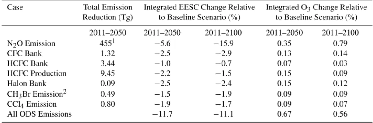
scenario and mitigation cases are shown in Fig. 1 for some of the most important compounds. All production of the chlorine- and bromine-containing ODSs shown is projected to be near zero by or before mid-century. This strongly lim-its the beneflim-its of any additional controls on future ODS production. The production of CFCs and halons is already very small, so the primary way to reduce emissions of these classes of ODSs involves capture and destruction of the banks. N2O projected emissions are different from those of
the ODSs in that the N2O emissions are projected to remain
near today’s values through the end of the century in the base-line scenario.
2.3 N2O and EESC
N2O has not been included in EESC calculations before.
There are important complications to including it because it participates in ozone destruction through the NOx cycle
rather than the ClOx or BrOx cycles. Increasing NOx
re-duces the efficiency of Clyand Bryfor ozone destruction by
tying up more of these halogens in the ClONO2and BrONO2
reservoir species. At elevated chlorine and bromine levels, this offsets some of the impact of an increase in N2O on
ozone depletion. Decreasing Clysimilarly ties up less NOy
in ClONO2, increasing the efficiency of N2O. These
inter-actions imply that the projected future decline in Cly and
Bry abundances, resulting from the Montreal Protocol
re-strictions, should lead to a greater impact of a unit change in N2O emissions on ozone (Ravishankara et al., 2009). On the
other hand, since the loss of stratospheric NOyis inversely
related to temperature, the efficiency of N2O for global ozone
depletion is expected to decrease as the upper stratosphere cools from the projected increases in CO2(Rosenfield and
Douglass, 1998). From the 2-D models considered here, we estimate that by 2100 this process will result in a decrease of 10–20% in the effectiveness of a unit N2O emission to lead
to ozone depletion compared with today. The effect of all of these interactions will potentially lead to a complicated rela-tionship between EESC and ozone depletion. Nevertheless, we will suggest an approach for including N2O in EESC here
and then quantify the success of this approach in Sect. 3. Fu-ture deviations of CO2 and EESC from the scenarios used
here will alter the extent of these interactions; however, the deviations are not expected to be significant enough to sub-stantively change the results.
Because our focus is on global ozone, we use the N2O
global ODP to quantify N2O’s contribution to EESC.
EESC(t )=fCFC−11· P Cl-containing compounds
nifCFCfi−11 ρi,entry−ρi(nat),entry
+α P
Br-containing compounds
nifCFCfi−11 ρi,entry−ρi,(nat),entry
+ξ ηnN2O
fN2O
fCFC−11 ρN2O,entry−ρN2O,(nat),entry (1)
whereαis the relative efficiency of bromine compared with chlorine for destroying total ozone andηis the same factor for nitrogen relative to chlorine when the nitrogen originates from N2O.ηis specifically for N originating from N2O
be-cause the efficiency of N production from N2O is included
in its value. ξ is a correction factor forηthat is discussed later,ni is the number of Cl, Br, or N atoms contained in
the ODS,fi is the fraction of the compound dissociated on
average in the stratosphere (assumed here to be for 3-yr-old age-of-air), andρi is the stratospheric entry mixing ratio in
pptv, assumed to equal the tropospheric mixing ratio for these gases. We consider only the anthropogenic contributions of N2O, CH3Br, and CH3Cl by explicitly subtracting the
tropo-spheric mixing ratio of each that arises from natural emis-sions (ρi,nat). All concentrations arising from natural
emis-sions are assumed to be constant in time, so we do allow the small increase in CH3Cl mixing ratios from WMO (2007) to
increase EESC.
If we use the semiempirical ODP formula (Solomon et al., 1992)
ODPi=η
ni
nCFC−11
fi
fCFC−11
τi
τCFC−11
MCFC−11
Mi
(2) it follows that
ηnN2O
fN2O
fCFC−11
=ODPN
2OnCFC−11
τCFC−11
τN2O
MN2O
MCFC−11
=6.4×10⁻³ (3)
where τi is the global lifetime of compound i, and Mi
is its molecular weight. Levels of ClOx and BrOx were
shown to significantly affect the N2O ODP in Ravishankara
et al. (2009); at 1959 levels, the ODP was calculated to be 0.026, compared with the 0.017 at 2000 conditions. We ac-count for this dependence on the N2O term by applying a
correction factor,ξ, in Eq. (1). This factor is assumed to be a linear function of the part of EESC arising from chlorine and bromine source gases so that the 1959 EESC level from these gases leads to a value forξof 1.53 (0.026/0.017) while the 2000 level of EESC leads to a value of 1.0. The 1959 and 2000 levels of EESC for the baseline scenario are 240 and 1640 pptv, respectively. This factor, along with Eq. (3), is then used in Eq. (1) to calculate N2O’s contribution to EESC.
The EESC/ozone depletion relationship of the N2O phaseout
case presented in Sect. 3 is more consistent with the other ODS cases whenξis included in Eq. (1).
2000 2020 2040 2060 2080 2100 0 100 200 300 400 500 600 ppt CFCs CFC-12 CFC-11 Bank Elimination Baseline
2000 2020 2040 2060 2080 2100 0 100 200 300 400 ppt HCFC-22 Baseline No Production Bank Elimination
2000 2020 2040 2060 2080 2100 Year 0 20 40 60 80 100 120 ppt CCl4 Baseline No Emission
2000 2020 2040 2060 2080 2100 Year 260 280 300 320 340 360 380 ppb
N2O
Baseline
No Emission
Fig. 1. Projected mixing ratios of N2O and selected ODSs for the baseline scenario and mitigation cases. Dotted curves (for CFCs and HCFC-22) represent mixing ratios assuming capture and de-struction of the entire 2011 bank. Dashed lines represent mixing ratios assuming elimination of future production beginning in 2011 for HCFC-22 and future emissions for CCl4and N2O.
By 2000, increases in CO2had already cooled the
strato-sphere and reduced the NOy/N2O ratio. Thus, when
calcu-lating ξ using the 1959 and 2000 ODPs, this effect is in-cluded. The temperature effect is expected to scale differ-ently with EESC in the future because EESC is projected to decrease while CO2 continues to increase in the A1B
sce-nario; thus, these interactions should lead to some additional error in the correlation between EESC from N2O and the
as-sociated ozone depletion. However, this error is smaller than the benefit gained from including the EESC dependence in this simplified manner. We note that quantifying N2O’s
con-tribution to EESC in this manner is appropriate for global ozone depletion only. The values forfN2O,fCFC−11,η, and
ξ would be different, for example, for the contribution of N2O to EESC relevant to the Antarctic ozone hole.
The age spectrum is applied to the EESC time series gener-ated from Eq. (1), equivalent to applying it to each entry mix-ing ratio before the summation is applied. EESC is generally calculated here assuming a 3-year mean age and an age spec-trum width of 1.5 years (Waugh and Hall, 2002) to represent the mean transport time between the troposphere and strato-sphere. Relative fractional release values for 3-year-old air from Newman et al. (2007) are assumed for all compounds except for HCFC-141b and HCFC-142b, which were charac-terized by high uncertainty in that analysis. The relative val-ues for these compounds are taken from WMO (2007). There has been discussion of a threshold in EESC below which changes in EESC have little or no impact on O3(e.g., Daniel
3 Results and discussion
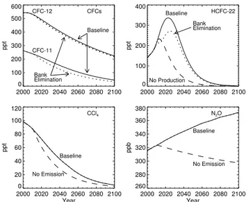
Figure 2 illustrates the maximum extent to which ODS and N2O emission phaseouts can accelerate the recovery of
ozone and EESC towards a state defined by the emissions of no ODSs or anthropogenic N2O at any time. Even with full
and immediate phaseouts of all ODS emissions, except for the three emission sources of CH3Br discussed in Sect. 2.1,
the recovery to the background case will not have occurred by 2100 because of the long residence times of several of the ODSs and N2O. Such a phaseout would, however, lead
to ozone levels that exceed ozone in the baseline case by 1.2–1.9% between 2030–2100. Chlorine and bromine emis-sion reductions would affect O3relatively quickly, with N2O
playing a larger role by 2100. To put this into perspective, relative to the background case, these models calculate a peak ozone depletion near 2000 of 7–8% for the baseline case and a depletion of about 4% by 2100. This peak depletion is substantially larger than the 3.5% quoted in WMO (2007) for the 2002–2005 time period because we are comparing to the higher O3 level calculated for the background case, which
includes increases in CO2and CH4 (and no ODSs), rather
than to the 1964–1980 average observed ozone level used in WMO (2007). It has been estimated that in the absence of the Montreal Protocol, and assuming continued growth of ODSs, globally-average total ozone depletion could have reached 17% by 2020 and 67% by 2065 when compared to 1980 levels (Newman et al., 2009). So while options still ex-ist to reduce future ozone depletion, the potential ozone im-pacts of additional controls are substantially reduced com-pared to what the Montreal Protocol has already achieved. Figure 2a also includes ground-based data from Fig. 3-2 in WMO (2007), allowing a comparison between the models and observations.
Figure 2a also shows the extent to which increases in CO2
and CH4 from the A1B scenario lead to higher calculated
column ozone in these two models. Total ozone’s return to 1980 levels is known to depend strongly on the future evo-lution of CO2 and likely on CH4(Portmann and Solomon,
2007; Chipperfield and Feng, 2003; Rosenfield et al., 2002; Randeniya et al., 2002). However, as stated in the introduc-tion, we do not consider CO2or CH4regulations to be
pol-icy options for reducing global ozone depletion. These gases are thought to have negative global ODPs, so their emissions would need to be increased to reduce ozone depletion. Such increases would lead to positive climate forcing.
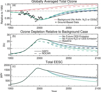
One metric used in ozone assessments to evaluate the im-pacts of ODS emissions reductions is the year when EESC drops below the 1980 level. Figure 2 shows that this time as-sociated with EESC, when calculated assuming a mean age of 3 y, does not perfectly indicate when total ozone deple-tion due to ODSs returns to 1980 levels and that the reladeple-tion- relation-ship is model dependent. For the 2-D models used here, the evolution of future total ozone depletion due to ODSs is ex-plained well by EESC, but EESC as calculated with a
differ-Globally Averaged Total Ozone
1950 2000 2050 2100
0.90 0.95 1.00 1.05
Relative to 1950 Ground-Based Data
(a)
Background (No Anthr. N2O or ODSs)
Ozone Depletion Relative to Background Case
1950 2000 2050 2100
0 10 20 30
DU
No Future N2O or ODS Emission
No Future ODS Emission
Baseline (b)
GSFC NOCAR
Total EESC
1950 2000 2050 2100
Year 0
500 1000 1500 2000
pptv
(c)
Fig. 2. (a)Globally averaged total column ozone, (b)ozone de-pletion relative to a case in which no anthropogenic N2O or ODSs were or will be emitted (“background” case), and(c)anthropogenic EESC time series including ODS and N2O contributions (calcu-lated assuming an age spectrum with a 3.0 y mean age, 1.5 y width). Cases shown are the baseline scenario (black), in which future ODS emissions follow a path consistent with current growth and Mon-treal Protocol controls and IPCC scenario A1B for N2O, CH4, and CO2; a case in which no anthropogenic ODSs are emitted after 2010 (blue); and a case in which no anthropogenic ODSs or N2O is emitted after 2010 (green). The ozone time series for the back-ground case is also shown (red). Solid lines are calculations from the GSFC model; dashed are for the NOCAR model. “+” symbols represent ground-based total ozone data (WMO, 2007) normalized so the 1964–1980 average agrees with the model calculations. The dotted lines represent the 1980 benchmark levels; 1980 values are used in previous ozone assessments and are also often considered in Montreal Protocol discussions. In panel (b), the NOCAR ozone depletion is increased by 3% so the depletion in 1980 is identical for the two models. For example, this leads to an apparent maximum depletion relative to the background case in the NOCAR model of 20.3 DU rather than the actual 19.7 DU.
1950 2000 2050 2100 Year
0.0 0.2 0.4 0.6 0.8 1.0
Normalized Ozone Depletion, EESC
Ozone EESC NOCAR (Mean Age=4.0 y)
GSFC (Mean Age=5.5 y)
Fig. 3. Comparison of normalized ozone depletion from NOCAR (blue) and GSFC (black) models with EESC (dashed). Ozone de-pletion for each model is normalized to the maximum dede-pletion, and EESC is normalized to its peak value. Age spectra used in the EESC calculations were determined by fitting the normalized EESC curves to the normalized ozone time series using a least-squares ap-proach. Mean ages derived for the EESC fits are shown. Age spec-tra widths were found to be 2.4 and 2.9 years, respectively, for the NOCAR and GSFC calculations. The older characteristic age for the GSFC model is apparent.
acceptable and useful metric, it may not perfectly describe the evolution of globally averaged total column ozone or the time when ozone depletion will reach some target level even in the absence of changes in CO2, CH4, or other non-ODS
emission or process. It is also important to recognize that the return of global total ozone to some approximately natu-ral level does not imply that the ozone profile, the latitudinal variations, or the radiative forcing associated with the strato-spheric ozone distribution will be the same as it was in the unperturbed state (WMO, 2007).
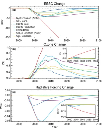
The effects of specific emissions reductions compared to the baseline scenario are quantified in terms of their effect on EESC, total ozone, and radiative forcing in Fig. 4. Ta-ble 1 also includes the effects on integrated EESC and ozone. Because each case involves an elimination of some future source of ODS emissions, the magnitude of the impact will be dependent on the amount of future emissions projected in the baseline scenario. For example, due to existing Mon-treal Protocol controls, by 2050 little emission remains in the baseline case for CFCs, Halons, CCl4, and HCFCs, with
specific details depending on the compound. This explains the general shape of increasing impacts in the short run and then decreasing impacts with time for most of the cases. The CH3Br phaseout leads to a nearly constant change in EESC
and ozone because of CH3Br’s short lifetime, combined with
the assumed continuing QPS emissions in the baseline sce-nario.
EESC Change
2000 2020 2040 2060 2080 2100
-150 -100 -50 0
pptv
(a)
N2O Emission (Anthr)
CFC Bank HCFC Bank HCFC Production Halon Bank CH3Br Emission (Anthr)
CCl4 Emission
Ozone Change
2000 2020 2040 2060 2080 2100
0.0 0.2 0.4 0.6 0.8 1.0
DU
(b)
2020 2040 2060 2080 2100 0.0
2.5 5.0
DU
Radiative Forcing Change
2000 2020 2040 2060 2080 2100
Year -0.05
-0.04 -0.03 -0.02 -0.01 0.00 0.01
W/m
2
(c)
2020 2040 2060 2080 2100 -0.30
-0.15 0.00
W/m
2
Fig. 4.Changes in(a)EESC,(b)total ozone from the GSFC model, and(c)radiative forcing, resulting from the various N2O and ODS reduction cases in Table 1. The responses for the N2O case (red) appear almost linear in the main panels because of its long lifetime and because future anthropogenic N2O emissions vary little through 2100 in the assumed A1B scenario. The insets in panels (b) and (c) have increased vertical scale ranges so the entire N2O change is visible through 2100. EESC is calculated assuming an average age of 3.0 y with an age spectrum width of 1.5 y.
The N2O anthropogenic emissions phaseout leads to
in-creasing impacts on EESC, ozone, and radiative forcing over the time period shown, a fundamentally different response than that of the ODSs. This response results from the long lifetime of N2O and from its continuing emission in the
base-line scenario, consistent with there being no current regula-tion that phases out its future emissions. Picking a longer time period will generally lead to greater relative importance of N2O emissions reductions compared with reductions of
ODSs. To illustrate the importance of the time horizon con-sidered, the integrated impacts in terms of EESC and ozone are shown for two time periods in Table 1. The larger rel-ative impact of the N2O reduction over the longer period
is clear. Of course, there is no scientific reason, and cur-rently no policy reason, to stop the integration at 2100, with ozone depletion still occurring relative to the background case. When dealing with a compound like N2O, whose
for evaluating policy options are similar to those encountered when evaluating the relative impacts of greenhouse gases on radiative forcing and climate. An important distinction dis-cussed below is that, unlike with climate change, it is pos-sible that we could return to natural globally-averaged total column ozone levels in the next few decades, albeit with large regional differences (e.g., depletion continuing in the tropics vs. recovery in the extratropics).
The year 1980 has frequently been used as a reference year to evaluate progress towards ozone recovery, but it likely does not mark the onset of global ozone depletion (Jackman et al., 1996) (also see Fig. 2). If no consideration is given to ozone depletion after total EESC returns to 1980 levels, a value judgment is made to neglect the importance of some emissions that could still deplete O3 several decades from
now. Choosing this threshold level and ignoring the con-tribution of N2O to EESC and ozone depletion in 1980, as
has been typically done in the past, further obscures the rele-vance of a return to 1980 EESC levels. A related question is whether there is a level of global column ozone above which anthropogenic ozone depletion is no longer considered im-portant. For example, if ozone column levels are still de-pleted due to the presence of ODSs, but they are higher than the globally-averaged natural level because of increases in CH4and CO2, is ozone depletion still a concern? If such an
acceptable level does exist, policy discussions will need to include the impact of future emissions of CO2and CH4on
ozone. Because of the relevance of climate policy to these future emissions, this could represent an important linkage between climate and ozone policy.
Figure 4 also shows that the capture and destruction of the CFC bank leads to a greater ozone change than the other chlorine- and bromine-containing ODS cases after about 2045, with an integrated ozone impact slightly larger than that of the Halon bank case from 2011–2100 (see Table 1). Even though the importance of these two banks to ozone is calculated to be similar, the Environmental Protection Agency estimates that in the United States of America the fraction of Halon banks that are technically accessible for capture and destruction (>95%) is much greater than the fraction of the CFC banks (<10%) (Montzka et al., 2008). Accessibility is an important factor in determining the cost of bank capture. We make this point to emphasize that our calculations only indicate the importance of various emission sources to ozone and climate forcing; we make no estimate of the costs or even the relative costs of reducing future emis-sions.
The complete phaseout of anthropogenic N2O emissions
leads to larger ozone and EESC changes than any other case considered from 2020–2025 onward, and its impact on inte-grated ozone and EESC from 2011–2100 is larger than all other cases combined. The relative importance of a phase-out in N2O emissions would become even greater beyond
2100. A phaseout of anthropogenic N2O emissions also has
the greatest impact on radiative forcing (Fig. 4c). By the
year 2100, an N2O phaseout would result in a radiative
forc-ing about 0.23 W/m2less than in the baseline scenario. The capture and destruction of the entire CFC bank would lead to a reduction of about 0.005 W/m2, and each of the other ac-tions would reduce radiative forcing by less than 0.001 W/m2 in 2100. In the shorter term, the HCFC bank and produc-tion cases lead to a radiative forcing change that is com-parable to that of the N2O case over about the next 5 and
10 years, respectively. Although an N2O phaseout currently
leads to the largest ozone and radiative forcing impacts of the cases considered, the Montreal Protocol has already resulted in large reductions in emissions of chlorine- and bromine-containing compounds. The associated reduction in direct radiative forcing due to the Protocol has been estimated to be 0.20–0.25 W/m2 by 2010 compared to a case assuming unregulated growth (Velders et al., 2007). However, some of this benefit could be negated by future increases in hy-drofluorocarbons (HFCs) used as replacements of CFCs and HCFCs (Velders et al., 2009).
In past ozone assessments, the impacts of additional ODS controls have been compared using EESC, integrated be-tween either 1980 or the current time and the return of EESC to 1980 levels. It has been assumed that the integrated EESC decrease is proportional to the integrated ozone increase. The results in Table 1, integrated from 2011–2050, are used to evaluate the validity of this assumption, and the results are shown graphically in Fig. 5. The individual points, represent-ing fractional EESC changes and fractional ozone changes, are not expected to fall exactly on a line because of known simplifications associated with the EESC formula and sin-gle values forη, α, andfi in Eq. (1) that do not perfectly
account for modeled processes that they are intended to rep-resent. As seen in Fig. 3, uncertainties in dynamics and re-sulting transport times can also play a role in the ability of EESC to accurately represent ozone depletion. Two of the largest differences in integrated ozone changes between the two models are for the CH3Br and Halon cases as evident in
Fig. 5. The lower impact on ozone depletion in the NOCAR model suggests that the representativeαvalue is somewhat lower than 60 for that model. Daniel et al. (1999) calculated a value of 45 using the NOCAR model, but revised kinet-ics rates since that study have acted to raise this value some (WMO, 2007). In spite of all the potential causes of an im-perfect relationship between EESC and ozone changes, the compact correlation shown in Fig. 5 demonstrates that the integrated ozone responses of the cases are represented quite well by the integrated EESC metric. The individual points for each model all fall within 30% of the linear fit for that model. If the age spectra from Fig. 3 are used instead of the mean of 3.0 y and width of 1.5 y, the best-fit slopes of the two models are less similar. In that case, the slope of the NOCAR model fit is about−0.04 while the slope of the GSFC model
fit is about−0.06. But more important, for each model the
-0.025 -0.020 -0.015 -0.010 -0.005 0.000 Fractional EESC Change
0.0000 0.0005 0.0010 0.0015
Fractional Change in O
3
Baselin CFC Bank
HCFC Bank HCFC Production
Halon Bank
CH3Br Emission
(Anthr)
CCl4 Emission
GSFC
NOCAR
-0.06 -0.04 -0.02 0.00 0.000
0.001 0.002 0.003 0.004
N2O Emission (Anthr)
Fig. 5. Correlation of integrated EESC changes (3 y mean age) with integrated globally averaged total column ozone changes over the period 2011–2050. Ozone values are calculated by the GSFC (filled diamonds) and NOCAR (squares) models. The linear fits of the cases shown are also included (solid for GSFC; dashed for NOCAR). These fits are forced to go through the origin and do not include the N2O case (red symbols) in their calculation. The NO-CAR slope (dashed blue) is less negative than the GSFC slope (solid black) primarily due to a smaller ozone change in the NOCAR bromine cases (green squares) than would be expected with anα
of 60. The inset shows the same information as the main figure with the scales expanded so the N2O emission phaseout case (red symbols) is visible.
The integrated EESC and ozone information from Table 1 is shown in an alternative way in Fig. 6. Here, the EESC change has been scaled by the slope of the line in the Fig. 5 fit to the GSFC results. If EESC were a perfect metric for eval-uating ozone depletion in the models shown and all the con-stants used in Eq. (1) were accurate, each ozone bar would be expected to be the same size as the corresponding EESC bar. The similar sizes of the same-colored bars in Fig. 6 fol-low directly from Figs. 4 and 5 and demonstrate the degree to which EESC is a good metric for ozone. The similar sizes of the ozone response bars for the two models demonstrate their good agreement. The ozone bars are slightly smaller relative to the EESC bars in the lower panel than in the upper panel. However, the relative sizes of the ozone bars are still in good agreement with the relative sizes of the EESC bars, evidence that EESC is a good metric for quantifying the rela-tive impacts of additional ODS controls on ozone during both of these time periods.
Integrated Scaled EESC and O3 Response
0.0 0.1 0.2 0.3 0.4
Percent Change
2011-2050
GSFC O3
NOCAR O3
EESC
(a)
0.0 0.2 0.4 0.6 0.8 1.0
Percent Change
2011-2100
N2O
Emission (Anthr)
CFC Bank
HCFC Bank
HCFC Prod
Halon Bank
CH3Br
Emission (Anthr)
CCl4
Emission
(b)
Fig. 6. Impact of the 7 hypothetical emissions reductions shown in Table 1 on integrated EESC (solid bars) and global total column O3from GSFC (horizontal hatching) and NOCAR models (angled hatching). Integration periods of(a)2011–2050 and(b)2011–2100 are shown. The EESC changes are scaled by the slope of the linear fit to the GSFC calculations (solid black line) shown in Fig. 5. The extent to which ozone bars are the same height as the same-colored EESC bars (in the same panel) quantifies the success of the EESC parameterization in describing the integrated ozone response.
4 Conclusions
Hypothetical reductions in future N2O and ODS emissions
from several potentially important sources have been ana-lyzed for their impact on EESC, globally averaged total col-umn ozone, and radiative forcing. The potential exists for accelerating future ozone increases and decreasing radiative forcing with additional ODSs and N2O controls. The impacts
on ozone are expected to be substantially smaller than those already accomplished by the Montreal Protocol.
We have presented an approach for including tropospheric concentrations of N2O resulting from anthropogenic
emis-sions into EESC. We have also demonstrated that integrated EESC is an effective proxy for integrated ozone changes for all emission reduction cases considered here, including the N2O case. Consistent with Ravishankara et al. (2009),
we have shown that a complete phaseout of anthropogenic N2O emissions would have a larger impact on stratospheric
ozone recovery than a combined phaseout of all anthro-pogenic chlorine- and bromine-containing ODSs when com-paring the integrated effects to 2100 and neglecting potential future growth in ODS feedstock uses and byproduct emis-sions. N2O emission reductions have a relatively larger
dependence on the time period considered raises the ques-tion of the level of concern devoted to ozone depleques-tion if global ozone increases above the natural level in the com-ing decades, for example due to increascom-ing CO2 and CH4,
but depletion at some latitudes and altitudes still occurs. Continuing anthropogenic N2O emissions assumed in the
IPCC A1B scenario also play a larger role in future direct ra-diative forcing from about 2030 onward than the combined sources of all the future ODS emissions examined here. In the long term, an elimination of anthropogenic N2O
emis-sions beginning in 2011 would reduce radiative forcing in 2100 by 0.23 W/m2, while the most significant ODS emis-sion reduction considered, the capture and destruction of the entire CFC bank, would lead to a reduction in radiative forc-ing of about 0.005 W/m2 in 2100. Over the next 5 and 10 years, respectively, the capture and destruction of the 2010 HCFC bank and the elimination of HCFC production from 2011 would lead to a radiative forcing change comparable to that of the N2O anthropogenic emission elimination.
In considering future N2O and ODS production or
emis-sion regulations, additional factors to those emphasized here will likely play a role as well, including for example, the economic cost associated with various regulations and the potential political tradeoffs of restricting some gases under the Montreal Protocol rather than under a climate agreement.
Acknowledgements. We appreciate the effort and comments of two
anonymous reviewers, who have helped improve the manuscript. We thank S. Solomon for helpful discussions and comments. We thank V. Fioletov for making the ground-based ozone data used in WMO (2007) available for us to include. E. L. Fleming and C. H. Jackman were supported by the NASA Atmospheric Composition: Modeling and Analysis (ACMA) Program. Work at NOAA was funded in part by NOAA’s Climate Program.
Edited by: W. Lahoz
References
Chipperfield, M. P. and Feng, W.: Comment on: Stratospheric ozone depletion at northern mid-latitudes in the 21st century: The importance of future concentrations of greenhouse gases nitrous oxide and methane, Geophys. Res. Lett., 30(7), 1389, doi:10.1029/2002GL016353, 2003.
Clarke, L., Edmonds, J., Jacoby, H., Pitcher, H., Reilly, J., and Richels, R.: Scenarios of Greenhouse Gas Emissions and At-mospheric Concentrations, Sub-report 2.1A of Synthesis and Assessment Product 2.1: Report by the U.S. Climate Change Science Program and the Subcommittee on Global Change Re-search, Department of Energy, Office of Biological & Environ-mental Research, Washington, DC, 154 pp., 2007.
Crutzen, P. J.: The influence of nitrogen oxides on the atmospheric ozone content, Q. J. Roy. Meteorol. Soc., 96, 320–325, 1970. Daniel, J. S., Solomon, S., and Albritton, D. L.: On the evaluation
of halocarbon radiative forcing and global warming potentials, J. Geophys. Res., 100(D1), 1271–1285, 1995.
Daniel, J. S., Solomon, S., Portmann, R. W., and Garcia, R. R.: Stratospheric ozone destruction: The importance of bromine rel-ative to chlorine, J. Geophys. Res., 104(D19), 23871–23880, 1999.
Denman, K. L., Brasseur, G., Chidthaisong, A., Ciais, P., Cox, P. M., Dickinson, R. E., Hauglustaine, D., Heinze, C., Holland, E., Jacob, D., Lohmann, U., Ramachandran, S., da Silva Dias, P. L., Wofsy, S. C., and Zhang, X.: Couplings between changes in the climate system and biogeochemistry, in: Climate Change 2007: The Physical Science Basis. Contribution of Working Group I to the Fourth Assessment Report of the Intergovernmental Panel on Climate Change, edited by: Solomon, S., Qin, D., Manning, M., Chen, Z., Marquis, M., Averyt, K. B., Tignor, M. and Miller, H. L., Cambridge University Press, Cambridge, UK and New York, USA, 2007.
Eyring, V., Waugh, D. W., Bodeker, G. E., Cordero, E., Akiyoshi, H., Austin, J., Beagley, S. R., Boville, B. A., Braesicke, P., Bruhl, C., Butchart, N., Chipperfield, M. P., Dameris, M., Deckert, R., Deushi, M., Frith, S. M., Garcia, R. R., Gettelman, A., Giorgetta, M. A., Kinnison, D. E., Mancini, E., Manzini, E., Marsh, D. R., Pawson, S., Pitari, G., Plummer, D. A., Rozanov, E., Schraner, M., Scinocca, J. F., Semeniuk, K., Shepherd, T. G., Shibata, K., Steil, B., Stolarski, R. S., Tian, W., and Yoshiki, M.: Multimodel projections of stratospheric ozone in the 21st century, J. Geo-phys. Res., 112, D16303, doi:10.1029/2006JD008332, 2007. Fleming, E. L., Jackman, C. H., Weisenstein, D. K., and Ko,
M. K. W.: The impact of interannual variability on multi-decadal total ozone simulations, J. Geophys. Res., 112, D10310, doi:10.1029/2006JD007953, 2007.
Jackman, C. H., Fleming, E. L., Chandra, S., Considine, D. B., and Rosenfield, J. E.: Past, present, and future modeled ozone trends with comparisons to observed trends, J. Geophys. Res, 101, 28753–28767, 1996.
Montzka, S. A., Daniel, J. S., Cohen, J., and Vick, K.: Current trends, mixing ratios, and emissions of ozone-depleting sub-stances and their substitutes, in: Trends in Emissions of Ozone-Depleting Substances, Ozone Layer Recovery, and Implications for Ultraviolet Radiation Exposure, edited by: Ravishankara, A. R., Kurylo, M. J., and Ennis, C. A., U.S. Climate Change Science Program and the Subcommittee on Global Change Research, De-partment of Commerce, NOAA’s National Climatic Data Center, Asheville, NC, 29–78, 2008.
Nakicenovic, N., Alcamo, J., Davis, G., de Vries, B., Fenhann, J., Gaffin, S., Gregory, K., Grubler, A., Jung, T. Y., Kram, T., La Rovere, E. L., Michaelis, L., Mori, S., Morita, T., Pepper, W., Pitcher, H., Price, L., Riahi, K., Roehrl, A., Rogner, H.-H., Sankovski, A., Schlesinger, M., Shukla, P., Smith, S., Swart, R., van Rooijen, S., Victor, N., and Dadi, Z.: Special report on emis-sions scnearios: A special report of working group III of the In-tergovenmental Panel on Climate Change, Cambridge University Press, Cambridge, UK, 599 pp., 2000.
Newman, P. A., Nash, E. R., Kawa, S. R., Montzka, S. A., and Schauffler, S. M.: When will the Antarctic ozone hole recover?, Geophys. Res. Lett., 33, 12, L12814, doi:10.1029/2005GL025232, 2006.
Newman, P. A., Oman, L. D., Douglass, A. R., Fleming, E. L., Frith, S. M., Hurwitz, M. M., Kawa, S. R., Jackman, C. H., Krotkov, N. A., Nash, E. R., Nielsen, J. E., Pawson, S., Stolarski, R. S., and Velders, G. J. M.: What would have happened to the ozone layer if chlorofluorocarbons (CFCs) had not been regulated?, At-mos. Chem. Phys., 9, 2113–2128, doi:10.5194/acp-9-2113-2009, 2009.
Pawson, S., Stolarski, R. S., Douglass, A. R., Newman, P. A., Nielsen, J. E., Frith, S. M., and Gupta, M. L.: Goddard Earth Ob-serving System chemistry-climate model simulations of strato-spheric ozone-temperature coupling between 1950 and 2005, J. Geophys. Res., 113, D12103, doi:10.1029/2007JD009511, 2008. Portmann, R. and Solomon, S.: Indirect radiative forcing of the ozone layer during the 21st century, Geophys. Res. Lett., 34(2), L02813, doi:10.1029/2006GL028252, 2007.
Randeniya, L. K., Vohralik, P. F., and Plumb, I. C.: Stratospheric ozone depletion at northern mid latitudes in the 21(st) century: The importance of future concentrations of greenhouse gases nitrous oxide and methane, Geophys. Res. Lett., 29(4), 1051, doi:10.1029/2001GL014295, 2002.
Ravishankara, A. R., Daniel, J. S., and Portmann, R.: Nitrous Ox-ide (N2O): The Dominant Ozone-Depleting Substance Emitted in the 21st Century, Science, 326, 5949, 123–125, 2009. Rontu Carlon, N., Papanastasiou, D. K., Fleming, E. L., Jackman,
C. H., Newman, P. A., and Burkholder, J. B.: UV absorption cross sections of nitrous oxide (N2O) and carbon tetrachloride (CCl4) between 210 and 350 K and the atmospheric implications, Atmos. Chem. Phys., 10, 6137–6149, doi:10.5194/acp-10-6137-2010, 2010.
Rosenfield, J. E. and Douglass, A. R.: Doubled CO2effects of NOy in a coupled 2D model, Geophys. Res. Lett., 25, 4381–4384, 1998.
Rosenfield, J. E., Douglass, A. R., and Considine, D. B.: The im-pact of increasing carbon dioxide on ozone recovery, J. Geophys. Res.-Atmos., 107(D5–6), 4049, doi:10.1029/2001JD000824, 2002.
Sander, S. P., Friedl, R. R., Golden, D. M., Kurylo, M. J., Moortgat, G. K., Wine, P. H., Ravishankara, A. R., Kolb, C. E., Molina, M. J., Finlayson-Pitts, B. J., Huie, R. E., and Orkin, V. L.: Chemical kinetics and photochemical data for use in atmospheric studies evaluation number 15, National Aeronautics and Space Adminis-tration, Jet Propulsion Laboratory, Pasadena, California, 523 pp., 2006.
Sherry, D.: HFC-23, CFC, and PCB management and disposal 2000–2010, A study undertaken for the World Bank, 2004. Solomon, S., Mills, M., Heidt, L. E., Pollock, W. H., and Tuck, A.
F.: On the Evaluation of Ozone Depletion Potentials, J. Geophys. Res., 97(D1), 825–842, 1992.
Solomon, S., Portmann, R. W., Garcia, R. R., Randel, W., Wu, F., Nagatani, R., Gleason, J., Thomason, L., Poole, L. R., and Mc-Cormick, M. P.: Ozone depletion at mid-latitudes: Coupling of volcanic aerosols and temperature variability to anthropogenic chlorine, Geophys. Res. Lett., 25(11), 1871–1874, 1998. SPARC CCMVal: SPARC CCMVal report on the evaluation of
chemistry-climate models, edited by: Eyring, V., Shepherd, T. G., and Waugh, D. W., SPARC Report No. 5, 2010.
TEAP: Task force decision XX/8 report, Assessment of alternatives to HCFCs and HFCs and update of the TEAP 2005 supplement report data, United Nations Environment Programme, Nairobi, Kenya, 2009.
Velders, G. J. M., Andersen, S. O., Daniel, J. S., Fahey, D. W., and McFarland, M.: The importance of the Montreal Protocol in protecting climate, P. Natl. Acad. Sci. USA, 104(12), 4814– 4819, 2007.
Velders, G. J. M., Fahey, D. W., Daniel, J. S., McFarland, M., and Andersen, S. O.: The large contribution of projected HFC emis-sions to future climate forcing, P. Natl. Acad. Sci. USA, 106(27), 10949–10954, 2009.
WMO: Scientific Assessment of Ozone Depletion: 1991, Global Ozone Research and Monitoring Project, Geneva, Switzerland, 25, 1991.
WMO: Scientific Assessment of Ozone Depletion: 1994, Global Ozone Research and Monitoring Project, Geneva, Switzerland, Report 37, 1995.
WMO: Scientific Assessment of Ozone Depletion: 1998, Global Ozone Research and Monitoring Project, Geneva, Switzerland, Report 44, 1999.
WMO: Scientific Assessment of Ozone Depletion: 2002, Global Ozone Research and Monitoring Project, Geneva, Switzerland, Report 47, 2003.