Present and future impact of aircraft, road traffic and shipping emissions on global tropospheric ozone

(1)

ACPD

10, 15755–15809, 2010

Present and future impact of transport emissions on global

tropospheric ozone

B. Koffiet al.

Title Page

Abstract Introduction

Conclusions References

Tables Figures

◭ ◮

Back Close

Full Screen / Esc

Printer-friendly Version Interactive Discussion

Discussion

P

a

per

|

Dis

cussion

P

a

per

|

Discussion

P

a

per

|

Discussio

n

P

a

per

|

Atmos. Chem. Phys. Discuss., 10, 15755–15809, 2010 www.atmos-chem-phys-discuss.net/10/15755/2010/ doi:10.5194/acpd-10-15755-2010

Atmospheric Chemistry and Physics Discussions

This discussion paper is/has been under review for the journal Atmospheric Chemistry and Physics (ACP). Please refer to the corresponding final paper in ACP if available.

Present and future impact of aircraft, road

tra

_ffi

c and shipping emissions on global

tropospheric ozone

B. Koffi1, S. Szopa1, A. Cozic1, D. Hauglustaine1, and P. van Velthoven2

1

Laboratoire des Sciences du Climat et de l’Environnement, UMR 8212, IPSL, CEA-CNRS-UVSQ, Gif-sur-Yvette, France

2

Royal Netherlands Meteorological Institute, KNMI, De Bilt, The Netherlands

Received: 30 May 2010 – Accepted: 3 June 2010 – Published: 28 June 2010 Correspondence to: B. Koffi(brigitte.koffi@lsce.ipsl.fr)

(2)

ACPD

10, 15755–15809, 2010

B. Koffiet al.

Title Page

Tables Figures

◭ ◮

Back Close

Full Screen / Esc

Discussion

P

a

per

|

Dis

cussion

P

a

per

|

Discussion

P

a

per

|

Discussio

n

P

a

per

|

Abstract

In this study, the LMDz-INCA climate-chemistry model and up-to-date global emission inventories are used to investigate the “present” (2000) and future (2050) impacts of transport emissions (road traffic, shipping and aircraft) on global tropospheric ozone. For the first time, both impacts of emissions and climate changes on transport-induced

5

ozone are investigated. The 2000 transport emissions are shown to mainly affect ozone in the Northern Hemisphere, with a maximum increase of the tropospheric column of up to 5 DU, from the South-Eastern US to Central Europe. The impact is dominated by road traffic in the middle and upper troposphere, north of 40◦_{S, and by shipping}

in the northern lower troposphere, over oceanic regions. A strong reduction of road

10

emissions and amoderate (B1 scenario) to high (A1B scenario) increase of the ship and aircraft emissions are expected by the year 2050. As a consequence, LMDz-INCA simulations predict adrastic decrease in the impact of road emissions, whereas aviation would become the major transport perturbation on tropospheric ozone, even in the case of avery optimistic aircraft mitigation scenario. The A1B emission scenario leads

15

to an increase of the impact of transport on zonal mean ozone concentrations in 2050 by up to₊30% and₊50%, in the Northern and Southern Hemispheres, respectively. Despite asimilar total amount of global NO_xemissions by the various transport sectors compared to 2000, the overall impact on the tropospheric ozone column is increased everywhere in 2050, due to a sectoral shift in the emissions of the respective transport

20

modes. On the opposite, the B1 mitigation scenario leads to asignificant reduction (by roughly 50%) of the ozone perturbation throughout the troposphere compared to 2000. Considering climate change, and according to scenario A1B, a decrease of the O₃ tropospheric burden is simulated by 2050 due to climate change (−1.2%), whereas an increase of ozone of up to 2% is calculated in the upper troposphere in the inter-tropical

25

(3)

ACPD

10, 15755–15809, 2010

B. Koffiet al.

Title Page

Tables Figures

◭ ◮

Back Close

Full Screen / Esc

Discussion

P

a

per

|

Dis

cussion

P

a

per

|

Discussion

P

a

per

|

Discussio

n

P

a

per

|

by 12% and by 4%, for the background and the transport-induced ozone, respectively. However, positive and negative climate e_ffects are obtained on ozone, depending on the season, region and altitude, with an increase of the transport-induced ozone per-turbation (+0.4 DU) in the already most affected area of Northern Hemisphere.

1 Introduction

5

Emissions from the transport sectors contribute globally for about 30% to 40% to global anthropogenic emissions of carbon monoxide and nitrogen oxides, respectively, and to about 25% of anthropogenic Non Methane Hydrocarbon Compounds, NMHCs (e.g., Olivier at al., 2005). In the atmosphere, CH₄, CO and NMHCs in presence of NO_xact as ozone precursors by forming radicals which finally contribute to the ozone

forma-10

tion (Crutzen et al., 1999) and therefore, indirectly impact on climate. Fuglestvedt et al. (2008) found that transport has contributed to 31% of the total man-made O₃ forc-ing, since preindustrial times. Unger et al. (2008) calculated that transport emissions in Europe and North America have a particularly large forcing and are therefore attrac-tive targets to counter global warming. The chemical production of ozone is a highly

15

non-linear function of emitted NO_x and NMHC precursors, and is very sensitivity to local meteorology and atmospheric background composition. Besides their e_ffect on the ozone concentration and its related radiative forcing, the emissions from transport also affect the OH concentration, i.e. the oxidizing capacity of the atmosphere (e.g., Niemeier et al., 2006). The emissions by the transport sector are expected to show

20

drastic quantitative and geographic changes in the next decades, which in turn will af-fect air quality and climate (Kahn Ribeiro et al., 2007). Moreover, significant changes in climate conditions are expected to occur in the future (Meehl et al., 2007), a_ffecting the atmospheric oxidation processes (Hedegaard et al., 2008), and thereby, possibly, the atmospheric perturbations induced by transport emissions.

(4)

ACPD

10, 15755–15809, 2010

B. Koffiet al.

Title Page

Tables Figures

◭ ◮

Back Close

Full Screen / Esc

Discussion

P

a

per

|

Dis

cussion

P

a

per

|

Discussion

P

a

per

|

Discussio

n

P

a

per

|

In the last decade, several atmospheric model studies were performed to assess the global impact of present-day transport emissions on the chemical composition of the atmosphere, but focusing on a given transport mode.

The impact of NO_xand CO current road emissions was first investigated by Granier and Brasseur (2003), who estimated their relative contribution between 12 and 15%

5

and of about 9% of the ozone background near the surface, in industrial and remote regions, respectively. More recently, Matthes et al. (2007) concluded that the maxi-mum relative impact of road tra_ffic emissions (NO_x, CO, NMHC) occurs at northern mid-latitudes in July, increasing the surface and the zonal mean ozone concentrations by up to 16% and 12%, respectively. They also demonstrated the important role of

10

NMHC that contribute to an indirect long-range transport of NO_x from road tra_ffic via the formation of PAN, and consequently, lead to a greater influence on ozone in remote areas (i.e., by+30%). Similar results were also obtained by Niemeier et al. (2006) who concluded that the road tra_ffic emissions increase the zonally averaged tropospheric ozone concentration by more than 10% in the boundary layer, and by about 6% at

15

500 hPa and 2.5% at 300 hPa, in July. Niemeier et al. (2006) and Matthes et al. (2007) reported changes in the July ozone surface concentration by 20% and by up to little more than 16% in source regions, respectively.

Many model studies investigated the present impact of international shipping on at-mospheric chemistry, and more specifically on ozone (Lawrence and Crutzen, 1999;

20

Corbett and Kohler, 2003; Dalsoren and Isaksen, 2006; Endresen et al., 2003, 2007; Eyring et al., 2005a, 2007 and references inside). They underlined that ozone per-turbations due to shipping is highly nonlinear, being most efficient in regions of low background pollution. These studies suggest an overall better ozone production e_ffi -ciency of NO_xship emissions, compared to road traffic emissions. However, they also

25

(5)

ACPD

10, 15755–15809, 2010

B. Koffiet al.

Title Page

Tables Figures

◭ ◮

Back Close

Full Screen / Esc

Discussion

P

a

per

|

Dis

cussion

P

a

per

|

Discussion

P

a

per

|

Discussio

n

P

a

per

|

of Global and European Transport Systems; http://www.pa.op.dlr.de/quantify/). They found that ship emissions contribute for a large part to surface ozone over the oceans (up to 40%), but also over some continental areas such as over Western America (15– 25%) and Western Europe (5–15%). A contribution up to 5–6% to the tropospheric ozone column was simulated over the North Atlantic.

5

The global impact of NO_xemissions from subsonic aircraft on ozone has been exten-sively investigated (Hauglustaine et al., 1994; Brasseur et al., 1996, 1998a; Wauben et al., 1997; Stevenson et al., 1997; Schumann, 1997; Schumann et al., 2000; Dameris et al., 1998; Kentarchos and Roelofs, 2002; Grewe et al., 2002; Gauss et al., 2006; Cari-olle et al., 2009). While representing less than 2% of the global current NO_xemissions,

10

the aircraft emissions are shown to lead to a significant ozone perturbation in the Up-per Troposphere and Lower Stratosphere (UTLS), i.e., where NO_xhave a much higher ozone production potential than at Earth’s surface, and where increases in ozone are known to cause an important radiative forcing (e.g., Sausen et al., 2005; Lee et al., 2009). First studies calculated for instance an increase by 2 up to 8% of the ozone

15

background (Brasseur et al., 1998a). However, large differences, in both magnitude and seasonality, were highlighted between the di_fferent studies, resulting notably from the lack of NMHC chemistry, the coarse vertical resolution at the tropopause, quanti-tative uncertainties on NO_x emissions by lightning and mass transport by convection (Grewe et al., 2002). More recently, Gauss et al. (2006) found a maximum increase

20

in the monthly averaged zonal mean ozone in June (₊7.6 ppbv) and a minimum in September (∼3 ppbv), and increase of 6 ppbv for July. Last results from the NMHC version of the LMDz-INCA model, using AERO2K 2002 emissions (Eyers et al., 2004) show lower changes and di_fferent spatial patterns, with a maximum perturbation of 3.5 ppbv in spring, and an increase of 2.6 ppbv for July (Cariolle et al., 2009). This

25

(6)

ACPD

10, 15755–15809, 2010

B. Koffiet al.

Title Page

Tables Figures

◭ ◮

Back Close

Full Screen / Esc

Discussion

P

a

per

|

Dis

cussion

P

a

per

|

Discussion

P

a

per

|

Discussio

n

P

a

per

|

For the first time, the combined effects of the three modes of transport and their re-spective influence on the current composition of the atmosphere have been recently investigated at the global scale, in the framework of the QUANTIFY project. A multi-model analysis based on 2000 preliminary road and aircraft (AERO2K 2002) emissions has been performed (Hoor et al., 2009). It provides a detailed interpretation of the

5

chemical and transport processes involved in the ozone and OH current perturbations by the three transport modes, and the related radiative forcing, as well as an assess-ment of uncertainties due to the di_fferent models formulation. While di_fferences were obtained in the magnitude of the impacts, similar results were simulated by the 6 global chemistry models involved (including LMDz-INCA), in terms of geographical patterns

10

and respective contributions by the di_fferent transport modes. The mean results are also consistent with previous studies for aircraft and shipping, whereas the predicted road perturbation was found to be lower than previously reported in the literature. The authors attributed the di_fferences to a significant under-estimation of the preliminary road emissions. Their study also highlighted that uncertainties between the models

15

are larger in summer than in winter, with a maximum zonal mean ozone perturbation at 250 hPa ranging from 3.5 ppbv for LMDz-INCA model to 6 ppbv for p-TOMCAT model, for July. In fact, the LMDz-INCA model is known to simulate relatively low tropospheric ozone production in summer compared to other models, due to particularly intense convection and associated dilution effect during this season.

20

While the impact of futures changes in anthropogenic emissions on background tro-pospheric ozone has been widely documented (e.g., for the most recent ones, Hauglus-taine et al., 2005; Gauss et al., 2006; Niemeier et al., 2006; Granier et al., 2006; Eyring et al., 2005b, 2007; Stevenson et al., 2006; Søvde et al. 2007; Wu et al., 2008), only few of them specifically dealt with transport emissions, mainly because no reliable

de-25

(7)

ACPD

10, 15755–15809, 2010

B. Koffiet al.

Title Page

Tables Figures

◭ ◮

Back Close

Full Screen / Esc

Discussion

P

a

per

|

Dis

cussion

P

a

per

|

Discussion

P

a

per

|

Discussio

n

P

a

per

|

in the United States. In the latter and most dramatic case, they calculated an increase by up to 50–100% (South Asia) of the surface ozone concentration compared to the present situation. Granier et al. (2006) analyzed the potential impact of changes in shipping routes in the Arctic region due to sea ice reduction induced by climate change. They found that the surface ozone concentration could increase during summertime to

5

ozone levels comparable to the values currently observed in many industrialized re-gions of Northern Hemisphere. Eyring et al. (2007) analysed the impact of a constant annual growth rate of 2.2% of ship emissions up to 2030. They found a contribution of 2030 shipping emissions of up to 8 ppbv and 1.8 DU for the annual mean near-surface ozone and the ozone column, respectively. Gauss et al. (2006) investigated the effects

10

of enhanced air tra_ffic along polar routes, and of potential changes in cruising altitudes. They concluded that an enhanced use of polar routes would lead to a significant in-crease in the zonal mean ozone concentration at high Northern latitudes in summer, but to a negligible e_ffect in winter. They also found that raising flight altitudes increases the ozone burden both in the troposphere and lower stratosphere, whereas lowering

15

the flight altitude has a contrasting effect depending on the altitude (decrease of ozone production in the UTLS and increase below). Finally, Søvde et al. (2007) used a 2050 NO_x global aircraft emissions dataset from the EU project SCENIC. They calculated that the subsonic aircraft emissions could be responsible for an increase by up to 10– 17 ppbv of O₃in annual/July zonal mean in the UTLS of the Northern Hemisphere.

20

In addition to changes in emissions, the global tropospheric chemistry will be a_ffected in the future by climate change (e.g., Hauglustaine et al., 2005; Isaksen et al., 2005; Brasseur et al., 2006; Liao et al., 2006; Murazaki and Hess, 2006; Stevenson et al., 2006; Grewe, 2007; Hedegaard et al., 2008; Wu et al., 2008). Most of the processes involved in the tropospheric chemistry depend notably on temperature, humidity and

25

(8)

ACPD

10, 15755–15809, 2010

B. Koffiet al.

Title Page

Tables Figures

◭ ◮

Back Close

Full Screen / Esc

Discussion

P

a

per

|

Dis

cussion

P

a

per

|

Discussion

P

a

per

|

Discussio

n

P

a

per

|

humidity and global radiation. Moreover, the liquid water content, the precipitation fre-quency and amount as well as the surface properties a_ffect wet and dry deposition lev-els. All the previous studies showed that future climate change will lead to an increase in water vapor and OH at global scale. This increase in OH within the troposphere will contribute to a significant change in the typical life time of many species, since OH is

5

participating in a large number of chemical reactions. As a result of enhanced water vapour, a decrease in future global ozone burden, but with positive and negative ozone changes according to altitude, season, model, and the reference year or the scenario are generally predicted (e.g., Wu et al., 2008, and references inside). Previous studies also showed that the changes in tropospheric ozone are not only dominated by

tro-10

pospheric chemistry, but also by the stratospheric ozone budget and its flux into the troposphere, which could increase by 2100 because of climate change (e.g., Hauglus-taine et al., 2005; Isaksen et al., 2005; Murazaki and Hess, 2006). Whereas all these previous studies focused on changes in the ozone background, the present study anal-yses the impact of climate change separately for the background ozone and for the

15

ozone generated by the transport emissions. The hypothesis here is that the above-mentioned climate-induced physical and chemical atmospheric changes will also have a significant influence on the impact of the emissions from the transport sector.

Since the tropospheric impact of transport emissions is expected to show important changes in the next decades, because of changes in both emissions and climate, it is

20

essential to assess such future changes, in order to implement adequate regulations and incentives. In this study, the LMDz-INCA model is used to study the impact of both present and future transport emissions, based on the QUANTIFY final updated emis-sion datasets. Our main objectives are (i) to quantify the contribution of each of the three sectors (road traffic, shipping and aircraft) to the ozone background

concentra-25

(9)

ACPD

10, 15755–15809, 2010

B. Koffiet al.

Title Page

Tables Figures

◭ ◮

Back Close

Full Screen / Esc

Discussion

P

a

per

|

Dis

cussion

P

a

per

|

Discussion

P

a

per

|

Discussio

n

P

a

per

|

Finally, conclusions are provided in Sect. 5.

2 The chemistry-climate model LMDz-INCA

The global Climate Chemistry Model LMDz-INCA consists of the LMDz (Laboratoire deM´et ´eorologie Dynamique) General Circulation Model (Sadourny and Laval, 1984; Le Treut et al., 1994, 1998), coupled with the chemistry and aerosol model INCA

(In-5

teraction with Chemistry and Aerosols) in order to represent the chemistry of the tro-posphere (Hauglustaine et al., 2004; Folberth et al., 2006).

The version of the LMDz model used here (LMDz 4.0) is described in Hourdin et al. (2006). It has 19 hybrid levels on the vertical from the ground to 3 hPa and a hori-zontal resolution of 2.5 degrees in latitude and 3.75 degrees in longitude (96×72 grid

10

cells). The large-scale advection of tracers is performed using the finite volume trans-port scheme of Van Leer (1977), as described in Hourdin and Armengaud (1999). The turbulent mixing in the planetary boundary layer is based on a second-order closure model. In the present study, the Emanuel scheme (Emanuel, 1991, 1993) was used for convection. The primitive equations in LMDz are solved in 3 min time-step, large-scale

15

transport of tracers is carried out every 15 min and physical processes are calculated at a 30 min time interval.

The INCA model is coupled on-line to the LMDz general circulation model. INCA considers the surface and 3-D emissions, calculates dry deposition and wet scavenging rates, and integrates in time the concentration of atmospheric species with a time step

20

of 30 min. INCA uses a sequential operator approach, a method generally applied in chemistry-transport-models (Muller and Brasseur, 1995; Brasseur et al., 1998b; Wang et al., 1998; Poisson et al., 2000). In addition to the CH₄-NO_x-CO-O₃ photochemistry representative of the tropospheric background (Hauglustaine et al., 2004), the non-methane hydrocarbon version of INCA used in this study (version NMHC.3.0) takes

25

(10)

ACPD

10, 15755–15809, 2010

B. Koffiet al.

Title Page

Tables Figures

◭ ◮

Back Close

Full Screen / Esc

Discussion

P

a

per

|

Dis

cussion

P

a

per

|

Discussion

P

a

per

|

Discussio

n

P

a

per

|

well as their photochemical oxidation products. For a more detailed description of the INCA-NMHC chemistry model, we refer to Folberth et al. (2006). A zonally and monthly averaged ozone climatology is prescribed above the tropopause (150 hPa), based on Li and Shine (1995). This climatology is deliberately kept fixed at present-day values in all simulations in order to isolate the e_ffects of tropospheric chemistry and climate

5

change to changes in the chemical composition of the stratosphere.

3 Modelling set-up

3.1 Emissions

The socioeconomic scenarios developed in the framework of the Intergovernmental Panel on Climate Change (IPCC) are commonly used as the reference to assess

10

the future global anthropogenic emissions. All the related SRES (Special Report on Emission Scenarios) emission estimates (Nakicenovic and Swart, 2000) project a global increase in emissions of ozone precursors by 2050, mainly because of eco-nomic growth in developing countries. Three of them (A1B, A1T and B1) show a

de-crease in these emissions in Europe and North America. However, these global

15

datasets, which are commonly used by the modellers’ community to assess the im-pact of the emissions by the di_fferent sectors on global chemistry and climate, do not provide transport sectoral details. Furthermore, assumptions about quantitative and geographic changes in emissions are rapidly evolving with emissions regulations, technological and market progress, and potential for non-fossil fuels. Therefore, an

20

update was required to assess how the impact from transport and from individual modes will be modified in future (Uherek et al., 2010). To this purpose, it is also of great importance to use realistic “present” and future emissions by other emis-sion sectors, since the ozone sensitivity to traffic emissions substantially depends on background precursor concentrations. All the “present” and future transport emissions

25

(11)

ACPD

10, 15755–15809, 2010

B. Koffiet al.

Title Page

Tables Figures

◭ ◮

Back Close

Full Screen / Esc

Discussion

P

a

per

|

Dis

cussion

P

a

per

|

Discussion

P

a

per

|

Discussio

n

P

a

per

|

project, as well as future non-traffic anthropogenic and the biomass burning emissions (www.pa.op.dlr.de/quantify/emissions). They consist in global files, with a resolution of 1◦

×1◦ longitude by latitude, for the years 2000 and 2050 and for two SRES marker scenarios (A1B and B1). The present non-traffic emissions are based on the latest release of the EDGAR 32FT2000 emission inventory for the year 2000 (van Aardenne

5

et al., 2005; Olivier et al., 2005). For biomass burning, monthly means for the year 2000 were used, based on the Global Fire Emissions Database GFEDv2 (van der Werf et al., 2006) with multi-year (1997–2002) averaged activity data, using Andreae and Merlet (2001) emission factors, updated for NO_x. The e_ffective injection height of biomass burning emissions into the atmosphere was taken into account with the

10

emission heights as prescribed by Dentener et al. (2006).

The biogenic emissions were calculated for 2000 with the dynamical global vege-tation model ORCHIDEE (Krinner et al., 2005), as described in Lathi ère et al. (2005). While these emissions might also show very important changes in future (e.g., Lathi ère et al., 2005; Lathi ère et al., 2006), high uncertainties still remain about their future

15

trends (Heald et al., 2009), so that no future global biogenic emission dataset can be provided for the different future IPCC scenarios. Therefore, they are fixed to the 2000 values in all our simulation experiments, such as oceanic emissions (Folberth et al., 2006).

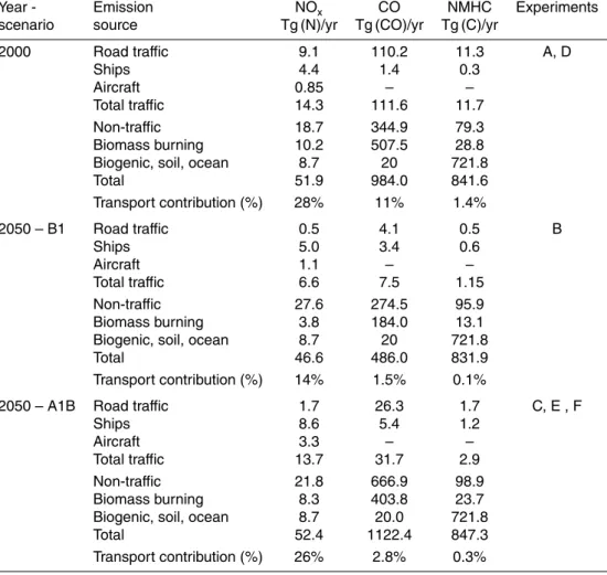
The resulting QUANTIFY 2000 final emissions from road (9.1 Tg NO_x(N)/yr, and

20

15 Tg NMHC/yr, 110 Tg CO) are significantly higher than QUANTIFY preliminary ones (6.85 Tg N/yr, and 10 Tg NMHC/yr, 73 Tg CO) used in Hoor et al. (2009). They are closer for NO_x, but still lower for CO and NMHC compared to previous assessments. For comparison, the road tra_ffic emissions adopted by both Matthes et al. (2005) and Niemeier et al. (2006) are 9 Tg (N)/yr and 36 Tg/yr for NO_x and NMHC, respectively.

25

(12)

ACPD

10, 15755–15809, 2010

B. Koffiet al.

Title Page

Tables Figures

◭ ◮

Back Close

Full Screen / Esc

Discussion

P

a

per

|

Dis

cussion

P

a

per

|

Discussion

P

a

per

|

Discussio

n

P

a

per

|

annual amount (0.85 Tg N) slightly higher but with very similar spatial distributions than AERO2K emission data.

The QUANTIFY transport emissions used in this study for A1B and B1 scenarios show very important changes in the future. Spatially, transport emissions shift in ab-solute amounts and relative shares from OECD countries to Asia, the Middle East and

5

South America (Uherek et al., 2010). Road tra_ffic emission fluxes strongly decrease at global scale, whereas a moderate (B1) to high (A1B) increase of the ship and aircraft emissions are expected by 2050 (Table 1). As shipping and aviation show strongest emissions in the future, increasing amounts of pollutants are emitted in the marine atmosphere and in the upper troposphere. As a result of changes in the use of the

10

di_fferent transport modes, as well as in fuel composition, consumption and e_fficiency, transport-induced emissions of NO_xdecrease by 20% (A1B) and 55% (B1) until 2050, whereas NMVOC and CO emissions decline by a factor 4 (A1B) to 10 (B1). As a re-sult from tra_ffic and non-tra_ffic emissions changes, the contributions of tra_ffic to NO_x, NMVOC and CO total emissions decrease from 28%, 1.4% and 11% in 2000 to 26%,

15

0.34% and 2.8% and to 14%, 0.14% and 1.5% in 2050 for A1B and B1 scenarios, respectively. For aircraft emissions, an additional scenario (B1ACARE) based on ex-cellent fuel e_fficiency is also investigated (Table 3).

3.2 The perturbation approach

A small perturbation approach is used to assess the impact of transport emissions on

20

global chemistry. For all studied scenarios, a reference simulation is first performed with all emissions. Then, the road tra_ffic, ship and aircraft emissions are separately reduced by 5% in 3 additional simulations. The total impact of transport emissions is calculated by adding the three perturbations rather than by simulating an additional per-turbation run for all transport emissions. Sensitivity tests performed with LMDz-INCA

25

(13)

ACPD

10, 15755–15809, 2010

B. Koffiet al.

Title Page

Tables Figures

◭ ◮

Back Close

Full Screen / Esc

Discussion

P

a

per

|

Dis

cussion

P

a

per

|

Discussion

P

a

per

|

Discussio

n

P

a

per

|

to the sum of the 3 perturbations due to a 5% reduction of each transport mode. The small perturbation approach minimizes non-linearity in atmospheric chemical e_ffects, which would occur by setting the respective emissions to zero. Furthermore, a small reduction in emissions is expected to be more realistic than a total decline.

Despite the non-linear character of the ozone perturbation, the 100% up-scaled

per-5

turbations (multiplied by a factor 20) are displayed on the figures, in order to better compare with the results of Hoor et al. (2009) and other previous studies using such up-scaling. In order to quantify the non-linear e_ffects, and to compare with previous studies using a total removal of emissions, a 100% decline of 2000 emissions was also simulated separately for each transport mode. Results (not shown) indicate that the

10

total removal of transport emissions induces an 8% higher transport-induced ozone burden perturbation, compared to the small perturbations subsequently rescaled to 100% (4.4%, 5.7% and 15.6% higher perturbations for shipping, aircraft and road traf-fic, respectively). At regional scale, di_fferences can reach up to 15%, 18% and 60% in zonal mean for road (boundary layer of Northern Hemisphere), aircraft (UTLS of

North-15

ern Hemisphere) and shipping (boundary layer of Northern Hemisphere), respectively. These results emphasize the need to always compare perturbations from a same mod-elling perturbation approach, as proposed in our study, and discussed in Grewe et al. (2010).

3.3 Experiments

20

3.3.1 Emission change experiments

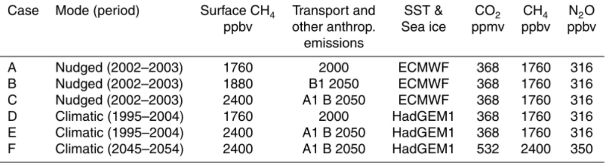
In order to assess the impact of 2000 to 2050 changes in emissions by each transport mode on the tropospheric chemical composition, five set of experiments (Table 2) were performed for present, and future (A1B and B1 scenario) emission datasets described in Table 1. Nudged runs over the 2002–2003 period, using the ECMWF operational

25

(14)

ACPD

10, 15755–15809, 2010

B. Koffiet al.

Title Page

Tables Figures

◭ ◮

Back Close

Full Screen / Esc

Discussion

P

a

per

|

Dis

cussion

P

a

per

|

Discussion

P

a

per

|

Discussio

n

P

a

per

|

al., 2009). The year 2002 was discarded to allow for the spin-up of the model and the year 2003 was analyzed. As described in Jourdain and Hauglustaine (2001), the Emanuel convection parameterization was used, which lead to a global annual NO production from lightning activity of about 5 Tg NO_x-N, which is similar to other studies (e.g., Lee et al., 1997; Prather et al., 2001).

5

In addition to the base runs reported in Table 2, corresponding 5% (and 100%) per-turbed runs were also performed. To account for the corresponding changes in CH₄ emissions, the CH₄ concentrations were prescribed as surface boundary conditions in the INCA model, on the basis of time-varying tropospheric mean mixing ratio of methane provided by the ENSEMBLES project (Hewitt and Griggs, 2004). A monthly

10

and latitudinal variability of CH₄ surface concentrations, based on observations from the AGAGE database was applied to these averaged mean ratios to account for the natural variability (J ¨ockel et al., 2006). An additional set of unperturbed/perturbed B1 scenario was also simulated in order to assess the impact of possible mitigation op-tions for aircraft, by reducing the NO_xaircraft emissions according to ACARE (Advisory

15

Council for Aeronautics Research in Europe; http://www.acare4europe.org/) targets for year 2050, as described in Table 3. These emission change experiments do not consider any climate change, which e_ffects are further analyzed through the climate change experiments, described in the following section.

3.3.2 Climate change experiments

20

Two 10 year periods (1995–2004 and 2045–2054) were simulated with the LMDz-INCA model in order to study the impact of climate change (Table 2). The three first years were discarded as the spin-up of the model and the 7 remaining years were averaged for each month of the year. Likewise the emissions change experiments, the impact of the transport emissions is assessed through a small perturbation approach (5%

25

(15)

ACPD

10, 15755–15809, 2010

B. Koffiet al.

Title Page

Tables Figures

◭ ◮

Back Close

Full Screen / Esc

Discussion

P

a

per

|

Dis

cussion

P

a

per

|

Discussion

P

a

per

|

Discussio

n

P

a

per

|

Firstly, the 2000 emissions were simulated in a present climate (Case D). Then, for both 10 year periods, the chemical emissions were fixed at 2050 level, in order to isolate the effect of climate change only (Cases E to F). The 2050 emissions from the A1B scenario were used. CO₂, CH₄ and N₂O green house gas concentrations were fixed in the LMDz model to 368 ppmv, 1760 ppbv and 316 ppbv and to 532 ppmv,

5

2400 ppbv and 350 ppbv, for “present” (2000) and future (2050) climates, respectively, on the basis of IPCC (2001). Transient climate simulation outputs from the Hadley Centre Global Environmental Model version 1 (HadGEM1) were used for sea-surface temperatures and sea ice (Stott et al., 2006). A 10-year averaging has been performed for each month separately to drive the LMDz model, over the 1995–2004 and 2045–

10

2054 periods.

The difference between D and E base runs gives an estimate of the impact of 2000– 2050 change in emissions in a present climate, whereas the impact of climate change is calculated from the di_fference between cases E and F. The E and F perturbed runs (5% reduction in transport emissions) provide an estimate of the impact of 2050 emissions

15

by the transport sector in a present and future climate, respectively. Finally, the change between the two latter impacts gives an estimate of the e_ffect of climate change on the impact of emissions by the transport sector between 2000 and 2050. It must be emphasized here that the ozone perturbation due to traffic emissions is not included in the climate perturbation, i.e., ozone changes do not feedback on climate.

20

4 Results and discussion

4.1 Impact of present-day transport emissions on the global tropospheric

chemistry

In this section, we assess the impact of present (2000) emissions by each of the three transport modes on tropospheric ozone from a 5% perturbation approach, based on

25

(16)

ACPD

10, 15755–15809, 2010

B. Koffiet al.

Title Page

Tables Figures

◭ ◮

Back Close

Full Screen / Esc

Discussion

P

a

per

|

Dis

cussion

P

a

per

|

Discussion

P

a

per

|

Discussio

n

P

a

per

|

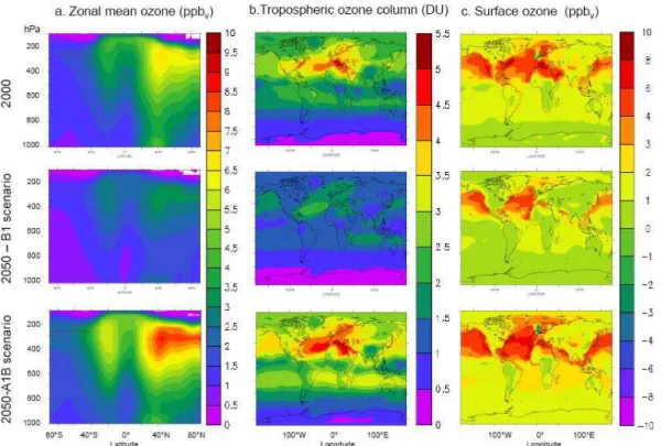
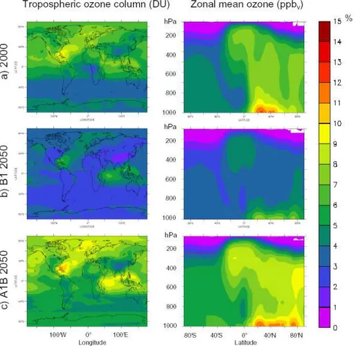
documented month in the literature. The ozone perturbations due to 2000 transport emissions (Case A) are shown in Fig. 1. The perturbation of the tropospheric ozone col-umn by all transport emissions is characterized by a strong hemispheric di_fference, with maximum effects in the Northern Hemisphere. A maximum impact is simulated over Europe and the Central Atlantic, reaching up 5 DU for the 100% up-scaled perturbation

5

(instead of 4.5 DU for LMDz-INCA preliminary simulations). The zonal mean ozone mixing ratio perturbation shows a maximum of 7 ppbv in the upper troposphere/lower stratosphere in the northern extra-tropics. At the surface, the total transport perturba-tion is also mainly concentrated over the Northern Hemisphere, with maxima of 8 ppbv over both land (over the eastern and western coasts of the US and over Arabia) and

10

sea (Mediterranean Sea) regions. Due to titration effect (Eyring et al., 2007), a slight ozone decrease is predicted under high NO_xconditions over the North Sea.

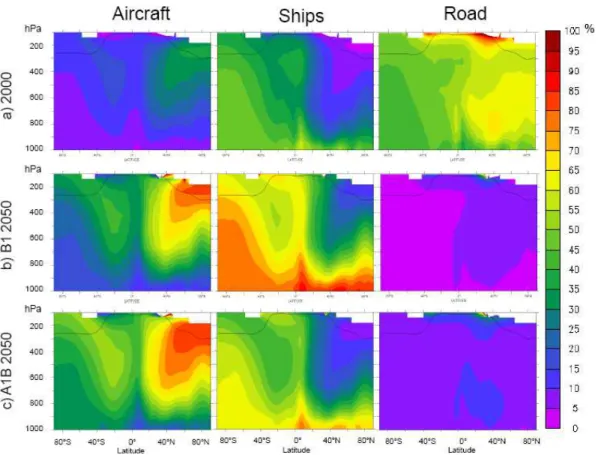
Figures 2, 3 and 4 show the relative contribution of each transport modes to the total transport-induced perturbation of the ozone tropospheric column, surface mixing ratio and zonal mean mixing ratio, respectively. The role of present-day road emissions

15

is highly dominant in comparison to the two other modes. It reaches up 85% over Asia, 75% over the US and 70% over Europe for the tropospheric column perturbation (Fig. 2). The relative contribution of road emissions to the ozone mixing ratio peaks in the free troposphere in both hemispheres, with a pronounced seasonal cycle in the northern extra-tropics, and a maximum in July. During summer, the boundary layer

20

mixing and convective transport into the free troposphere of the road tra_ffic emissions are more vigorous (Hoor et al., 2009). This explains the obtained seasonal cycle of the perturbation and why a high impact of road emissions is not only predicted in the boundary layer over land, where it accounts for up to 95% of the total perturbation (Fig. 3), but also in the free troposphere (Fig. 4). Land-based emissions account for

25

up to 70% and 60% of the total zonal mean perturbation in the mid and northern high troposphere. North of 40◦_{S, the contribution of shipping emissions to the ozone}

(17)

ACPD

10, 15755–15809, 2010

B. Koffiet al.

Title Page

Tables Figures

◭ ◮

Back Close

Full Screen / Esc

Discussion

P

a

per

|

Dis

cussion

P

a

per

|

Discussion

P

a

per

|

Discussio

n

P

a

per

|

are the major perturbation in both hemispheres (i.e.>50% and>40% of the total trans-port perturbation, respectively), with a maximum share of 60% at the equator latitude. The impact is mainly located over marine regions, islands and coastal areas (Fig. 3). Despite much lower emission levels than for ships and road traffic, NO_xemitted by avi-ation also lead to a significant increase of ozone in the upper troposphere. This is due

5

to higher ozone production e_fficiency than for the two other modes. The LMDz-INCA results for QUANTIFY aircraft emissions (0.85 Tg (N)/yr) are qualitatively and quanti-tatively close to those obtained for AERO2K emissions (0.67 Tg N/yr). The maximum perturbation mainly lies from 250 to 350 hPa and 40◦ _{to 70}◦_{N, which corresponds to}

the North Atlantic Flight Corridor. Maximum perturbations of 2.5 and 2.4 ppbv are,

re-10

spectively obtained in the UTLS of Northern Hemisphere, corresponding to 40% of the total transport perturbation in this area for July (Fig. 4). The impact in the lower tropo-sphere (<10% in zonal mean; Fig. 4) and at the surface (<15% over most of the globe; Fig. 3) is low, except over Northern Asia, where it reaches up 30% of the total surface perturbation by the three transport modes.

15

Figure 5 shows the ozone perturbation to the combined emissions from the different transport sectors. As for Fig. 1, the 100% up-scaled perturbations are displayed to better allow the comparison with Hoor et al. (2009). The perturbation ranges from 4 to 9% (Western Europe, Indian Ocean, Southern Asia) and 10% (Mexico Gulf) for the ozone column, north of 20◦_{S in July (Fig. 5), and throughout the year (not shown). In}

20

the southern extra-tropics, the perturbation is less than 5%. The relative perturbation to the zonal mean ozone ranges from 4 to 8% in the UTLS in the Northern Hemisphere, and up to 13% in the boundary layer. The perturbation in the Southern Hemisphere is about 4–5% in the low and middle troposphere (below 500 hPa) and of 2–3% above.

Hereafter, we compare our simulations results from a total removal of emissions from

25

(18)

ACPD

10, 15755–15809, 2010

B. Koffiet al.

Title Page

Tables Figures

◭ ◮

Back Close

Full Screen / Esc

Discussion

P

a

per

|

Dis

cussion

P

a

per

|

Discussion

P

a

per

|

Discussio

n

P

a

per

|

layer, 5% at 500 hPa and 4% at 300 hPa, in the Northern Hemisphere. These results are consistent with Niemeier et al. (2006) who reported very similar spatial patterns, and slightly higher perturbations (up to 10%, 6% and 5%, respectively). Matthes et al. (2007) results are somewhat larger (up to 12%, 8% and 6%, respectively). As pre-viously mentioned, both previous studies used similar total road emissions for NO_x,

5

but higher amounts for CO and NMHC than in the present work. Removing all ship-ping emissions leads to a decrease in the near-surface zonal mean of up to 3.2 ppbv and 1.8 ppbv at northern mid-latitudes for July and annual zonal means, respectively. A relative contribution up to 5% (over Asia) and 50% (corresponding to over the North Pacific) to the ozone column and surface ozone are calculated, respectively. These

10

results are of the same order of magnitude than in Eyring et al. (2007): using 30% lower NO_x emissions from shipping, this multi-model study reported an increase in near-surface annual and zonal mean O₃up to 1.3 ppbv, ranging from 1.0 (LMDz-INCA) to 1.9 ppbv, according to the model. They obtained a maximum increase of about 12 ppbv (modeled ensemble mean) over the North Atlantic for July, whereas we

ob-15

tain up to 8 ppbv and 9 ppbv over the Atlantic and Pacific oceans, respectively. Our results are closer to Dalsoren et al. (2009), who calculated a contribution of the ship emissions of up to 5–6% to the tropospheric ozone column (over the North Atlantic) and up to 40% to the surface ozone (over the North Pacific) for 2004 shipping emis-sions. As previously mentioned, Dalsoren et al. (2009) also used updated QUANTIFY

20

emissions, but for 2004 (10% more NO_xthan in 2000 QUANTIFY emissions). In both cases, the Northern Pacific is the most impacted region, whereas Eyring et al. (2007) obtained a much lower impact over the Pacific (<4 ppbv for the ensemble mean) com-pared to the Atlantic (up to 12 ppbv). This can explain the lower surface zonal mean O₃perturbation (1.3 ppbv against 1.8 ppbv) obtained in this previous study, which was

25

(19)

ACPD

10, 15755–15809, 2010

B. Koffiet al.

Title Page

Tables Figures

◭ ◮

Back Close

Full Screen / Esc

Discussion

P

a

per

|

Dis

cussion

P

a

per

|

Discussion

P

a

per

|

Discussio

n

P

a

per

|

the lower range of the perturbations reported in Hoor et al. (2009) for July. Our results for a total removal of QUANTIFY aircraft emissions lead to similar results, with a maxi-mum zonal-mean perturbation of 2.6 ppbv in the UTLS of Northern Hemisphere, which is significantly lower than the perturbation of 6 ppbv obtained by Gauss et al. (2006). One reason for such discrepancies is the strong dilution e_ffect due to particularly high

5

convection and mixing calculated by the LMDz-INCA model in summer, which induces lower ozone perturbations from aircraft and shipping compared to other models, and a maximum in spring.

4.2 2000 to 2050 changes in the impact of transport emissions

In this section, we assess the effect of future changes in traffic emissions on

tropo-10

spheric ozone. The simulations have been performed for two different scenarios (Ta-ble 2). As previously, the 100% up-scaled perturbations are shown (see Sect. 3.2). Ex-cept where stated, the results in this section are mainly discussed in terms of 2000 to 2050 relative change in the transport-induced ozone perturbation rather than in terms of absolute perturbation. The impact of emissions from each transport mode, and from

15

all transport emissions are firstly reported. The sensitivity of the results to possible mitigation options is then discussed.

4.2.1 A1B and B1 emission scenarios

Based on the QUANTIFY future emissions, we assume a high reduction of road emis-sions, and a moderate (B1 scenario) to high (A1B scenario) increase of ship and aircraft

20

emissions in 2050. As a consequence, the contribution of road traffic to the O₃column perturbation drastically decreases in 2050, accounting for less than 15% of the total transport perturbation over most of the globe, for both scenarios (Fig. 2). Ship emis-sions become the predominant contribution to the O₃column perturbation in the South-ern Hemisphere, especially for the B1 scenario, for which it contributes up to 85% to

25

(20)

ACPD

10, 15755–15809, 2010

B. Koffiet al.

Title Page

Tables Figures

◭ ◮

Back Close

Full Screen / Esc

Discussion

P

a

per

|

Dis

cussion

P

a

per

|

Discussion

P

a

per

|

Discussio

n

P

a

per

|

lower troposphere in the Northern Hemisphere (Fig. 4). Their influence remains mainly located over marine regions, whereas aircraft have the strongest impact on ozone in the continental boundary layer (Fig. 3). Nevertheless, in the case of the B1 scenario, the impact of shipping on surface ozone extends more inside the continents, because of the synoptic transport of ozone and its precursors inland. The surface ozone

per-5

turbation due to ship emissions in the most a_ffected coastal regions increases from about 2 ppbv in 2000 to 3 ppbv. In both future scenarios, subsonic aviation becomes the major ozone perturbation in the Northern Hemisphere, by contributing up to 70% and 75% to the total transport perturbation over the US, and up to 80% and 85% over continental Asia, for B1 and A1B scenarios, respectively (Fig. 2).

10

In the case of the B1 scenario, the decreased transport emissions lead to a signifi-cant reduction (by roughly 50%) of the ozone perturbation throughout the troposphere in 2050 (Figs. 1 and 5). At the surface, an even more pronounced decrease of the perturbation is simulated over land, due to the drastic reduction in road emissions. The total (up-scaled) surface ozone perturbation over Western Europe drops from 6 ppbv

15

to less than 2 ppbv (Fig. 1c). For the same reason, the combined impact of traffic decreases over the oceans, despite a slight increase in ship emissions (from 4.39 to 5.05 Tg N/yr). Despite similar total NO_xtransport emission in 2050 compared to 2000 (i.e., 14.3 against 14.1 Tg (N)/yr), the A1B scenario leads to an increase of the impact of transport on ozone by up to+30% and+50% in the Northern and Southern

Hemi-20

spheres, respectively (Figs. 1 and 5). The increase is even more pronounced in the UTLS region in the Northern Hemisphere. This is mainly due to a high increase in aircraft emissions (from 0.8 to 3.3 Tg (N)/yr), and to their high ozone production effi -ciency. In the lower troposphere, in the Northern Hemisphere, the relative perturbation increases by 2050 according to scenario A1, but to a lesser extent than in the upper

25

(21)

ACPD

10, 15755–15809, 2010

B. Koffiet al.

Title Page

Tables Figures

◭ ◮

Back Close

Full Screen / Esc

Discussion

P

a

per

|

Dis

cussion

P

a

per

|

Discussion

P

a

per

|

Discussio

n

P

a

per

|

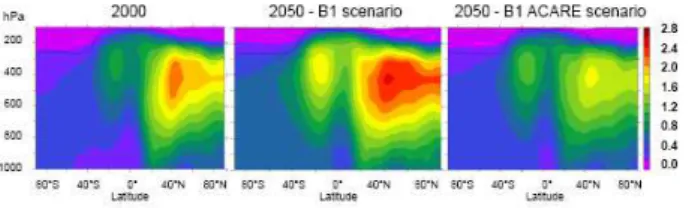
4.2.2 B1 ACARE mitigation

In order to assess the efficiency of possible emission reduction strategy in view of limiting the future impact of aircraft, the B1 ACARE scenario has been simulated for 2050. It corresponds to B1 2050 emission scenario, but with a reduction of the aircraft emissions due to the implementation of ACARE targets (Table 3). The scenario is

char-5

acterized by the lowest NO_x global aircraft emissions, i.e., even lower than the 2000 emissions. It can be seen as a more restricting but technically feasible scenario. The ozone perturbation due to aircraft emissions for the B1 2050 ACARE scenario is illus-trated and compared to 2000 and B1 2050 perturbations in Fig. 6. A 5% perturbation of aircraft emissions leads to a perturbation of less than 0.10% of the zonal mean ozone

10

background of the upper troposphere of Northern Hemisphere, instead of up to 0.12% and 0.14% for 2000 and B1 2050 emissions, respectively (Fig. 6a). The ozone column perturbations show that the implementation of the B1 ACARE 2050 targets leads to a decrease of 25% to 36% of the impact of aviation compared to B1 2050 (not shown). The higher relative effect is simulated over the Southern Hemisphere and around the

15

equator. As a consequence, whereas for B1 scenario, the aircraft impact increases over most of the globe from 2000 to 2050 (except over a region including South of US and a Western part of the North-Atlantic ocean), the B1 ACARE scenario leads to an increase in the Southern Hemisphere (by up₊30%), but a decrease in the Northern Hemisphere (by down to−30%) compared to 2000 (Fig. 6b). Aviation still remains the

20

major transport contributor to the ozone perturbation in the Northern Hemisphere, by contributing by up to 70% to the transport perturbation on the O₃column (not shown), instead of 85% for the B1 scenario without mitigation (Fig. 2b).

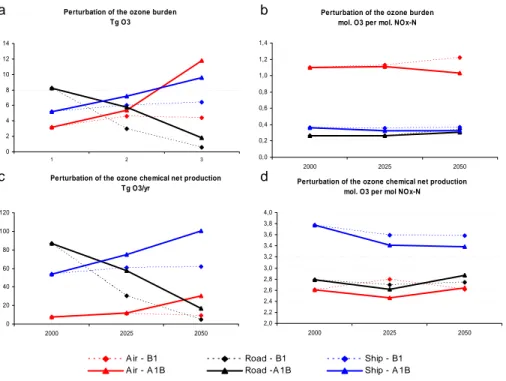
Figure 7a shows the sensitivity of the global ozone burden to each transport mode, for 2000, 2025 and 2050 emissions. The predominant perturbation mode shifts from

25

(22)

ACPD

10, 15755–15809, 2010

B. Koffiet al.

Title Page

Tables Figures

◭ ◮

Back Close

Full Screen / Esc

Discussion

P

a

per

|

Dis

cussion

P

a

per

|

Discussion

P

a

per

|

Discussio

n

P

a

per

|

highly modified, despite changes in the background chemical composition (Fig. 7b). In agreement with Hoor et al. (2009), aircraft NO_x emissions have an ozone production e_fficiency about three times higher than road tra_ffic and shipping. In fact, aircraft emit directly into the UTLS, where NO_x and ozone have a longer lifetime and accumulate, so leading to larger and more persistent perturbations compared to the Earth’s

sur-5

face, where the exhaust products are more rapidly removed by scavenging and dry deposition (e.g., Hauglustaine et al., 2005; Gauss et al., 2006; Dahlmann et al., 2009), However, as already mentioned, the shipping emissions have the highest net chemical production per NO_x molecule (Fig. 7c). This is due to the fact these emissions largely occur in low polluted environments. Our results are also in accordance with Dahlmann

10

et al. (2009) who found that future changes in ozone production by the transport sector strongly depend on the respective contributions of the three transport modes (because of their different ozone production efficiency), whereas changes in the atmospheric background composition only slightly modify the ozone production e_fficiency from each source.

15

4.3 Influence of climate change

In this part, we present the impact of transport emissions, in the context of climate changes for the A1B 2050 emission scenario. The e_ffect of climate change on the future meteorological and chemical states of the troposphere is first presented. It is compared to available published results, which mainly concerned scenario A2 and

20

year 2010. The innovative investigation of the changes in the transport-induced ozone perturbation due to climate change is then presented.

4.3.1 Change in global climate and tropospheric chemical composition

The 2000–2050 climate change and its impacts on the background chemical compo-sition of the troposphere is based on the di_fferences between H and G simulations

25

(23)

ACPD

10, 15755–15809, 2010

B. Koffiet al.

Title Page

Tables Figures

◭ ◮

Back Close

Full Screen / Esc

Discussion

P

a

per

|

Dis

cussion

P

a

per

|

Discussion

P

a

per

|

Discussio

n

P

a

per

|

The change in the global mean annual surface temperature (₊1.3◦_{C) as simulated}

by the LMDz-INCA model between the two time-slice periods is consistent with the last IPCC results (Meehl et al., 2007), which reported a 2000–2050 surface warming of

+1.4◦_{C for A1B emission scenario, from an ensemble of 21 models. Surface}

tempera-ture changes less than 4◦_{C are predicted in annual mean over most of the globe. A}

sim-5

ilar change is also generally predicted for January and July (not shown), but reaching locally up to 9◦_{C (e.g., over the US and Eastern Russia). The zonal mean}

tempera-ture increases by up to 2.5◦_{C throughout the troposphere in July. Lower changes are}

obtained in January south to 40◦_{N, but higher ones more North (Fig. 8a). An}

asso-ciated increase in water vapor is obtained in most of the troposphere, reaching up to

10

+60% in zonal mean in the UTLS region (Fig. 8b). These changes in temperature and water vapor are consistent with previous studies. For instance, Brasseur et al. (2006) predicted similar, but stronger changes (up to 150% for the water vapor) by July 2100 for the more pessimistic A2 scenario, using ECHAM5/OM-1 model. The 2000–2050 changes in precipitation rate (not shown) simulated in our study also show similar

gen-15

eral trends (decrease in tropical Atlantic and increase in tropical Pacific) compared to the 2000–2100 precipitation change simulated by Brasseur et al. (2006) for A2 sce-nario. As a result of enhanced water vapour, a decrease in future global ozone burden is generally predicted, since more water vapor leads to more ozone loss through O1(D) reaction with H₂O (Stevenson et al., 2006). However, both positive and negative ozone

20

changes are reported according to the altitude, the season, the model, the reference year or the scenario (e.g., Hauglustaine et al., 2005; Murazaki and Hess, 2006; Wu et al. 2008). Figure 9a shows the calculated 2000–2050 changes in the ozone, NO_x and CO zonal means for scenario A1B, in January and July. We obtain similar spa-tial patterns, but logically lower magnitude of changes compared to the 2000–2100

25

(24)

ACPD

10, 15755–15809, 2010

B. Koffiet al.

Title Page

Tables Figures

◭ ◮

Back Close

Full Screen / Esc

Discussion

P

a

per

|

Dis

cussion

P

a

per

|

Discussion

P

a

per

|

Discussio

n

P

a

per

|

in the chemical production (not shown). In addition to these processes, the decrease of ozone also predicted in the lower troposphere (below 800 mb) around 20◦_{N and}

20◦_{S in July and January, respectively, is due to a shorter lifetime of ozone and}

per-oxyacetylnitrate (PAN) at warmer temperatures (Wang et al, 1998; Hauglustaine et al., 2005; Brasseur et al., 2006; Wu et al., 2008). This process would allow explaining the

5

associated increase in NO_x concentrations (Fig. 9b) and the strong positive change in ozone chemical net production at these altitudes (not shown). According to the latter previous studies, the larger ozone decrease (up to 6–10%) predicted in the upper tro-posphere (∼300 hPa) could also reflect the elevation of the tropopause height due to climate change (see also Collins et al., 2003).

10

In a warmer climate, the hydrological cycle is more active and the convection en-hanced. Such an increase in convection and the related lightning NO_xproduction were shown to have a strong impact on NO_x background concentrations, and thus on the magnitude of the anthropogenic perturbations on upper tropospheric ozone. On one hand, it was shown to lead to a higher production of lightning NO_x, and thus to an

15

increase in NO_x and ozone concentrations, especially in the tropics (Hauglustaine et al., 2005; Zhao et al. 2009). On the other hand, the stronger vertical mixing due to convection reduces the NO_x background concentrations in the upper troposphere of extra-tropical regions, and consequently to increase the production ozone efficiency of aircraft NO_x emissions. Results from our simulations show an increase by up to 25%

20

in NO_x background concentrations in the upper troposphere over the inter-tropical re-gion (Fig. 9b). This climate-induced increase is due to the NO_xproduction by lightning, which is shown to increase by 7.3% at global scale because of enhanced convection, from 4.67 to 4.84 Tg NO_x-N. As a consequence, the zonal mean ozone concentration increases by up to 4% in the UTLS in this region. Inversely, in the extra-tropical

lati-25

(25)

ACPD

10, 15755–15809, 2010

B. Koffiet al.

Title Page

Tables Figures

◭ ◮

Back Close

Full Screen / Esc

Discussion

P

a

per

|

Dis

cussion

P

a

per

|

Discussion

P

a

per

|

Discussio

n

P

a

per

|

4.3.2 Change in the impact of transport on tropospheric chemistry

In this section, we assess the effect of climate change on the impact of future traffic emissions on tropospheric ozone, from present (Case E) and future (Case F) base and perturbation runs (Table 4). As done in the previous section, the transport perturbations were assessed by a 5% perturbation of emissions, subsequently up-scaled to 100%.

5

While this approach was shown to under-estimate by 8% the global transport-induced ozone perturbation, it does not significantly a_ffect the evaluation of its changes due to climate change, since it was applied to both present and future climates. The simulated impact of 2000 (Fig. 10a) and A1B 2050 (Fig. 10b) transport emissions on the ozone column in a present climate are consistent with the results previously obtained from

10

2003 meteorological runs (Fig. 1a). Similar spatial patterns but slightly lower perturba-tions are obtained for these climatic runs. The general patterns of the impact of A1B 2050 transport emissions on the ozone column are very similar in the future (Fig. 10c) and present (Fig. 10c) climate. In both cases, an increase in the ozone column is predicted, with (up-scaled) maxima of +5.0 DU (January) and +5.5 DU (July) in the

15

Northern Hemisphere. In July, the most impacted area (>4.0 DU) mainly extends from the Eastern US to Eastern Europe, and also includes a large part of the Mediterranean region. In January, Asia and the North Pacific Ocean also experience an increase by up to₊5.0 DU (present climate) and₊4.5 DU (future climate). The perturbation of the ozone zonal mean mixing ratio (not shown) reaches ₊9 (and ₊9) ppbv in the upper

20

troposphere of the Northern Hemisphere in July, and+7.5 (and+8.0) ppbv in January, for the present (and future) climates. These results are consistent with the nudged sim-ulations results, which showed that this high impact of 2050 transport emissions in the upper troposphere in the Northern Hemisphere was due for a large part to the aircraft emissions and their high ozone production efficiency (Figs. 4 and 5).

25

(26)

ACPD

10, 15755–15809, 2010

B. Koffiet al.

Title Page

Tables Figures

◭ ◮

Back Close

Full Screen / Esc

Discussion

P

a

per

|

Dis

cussion

P

a

per

|

Discussion

P

a

per

|

Discussio

n

P

a

per

|

change. A climate-induced increase of up to+0.6 DU is simulated in January in both Northern (North Pacific) and Southern (West Coast of South-America) Hemispheres (Fig. 11a). In July, the climate change enhances the e_ffect of transport emissions in the already most impacted zone, by up to 0.4 DU (i.e, by +10%) in the Gulf of Mex-ico (Fig. 11b). In Western Europe, an increase reaching up 0.3 DU (July) and 0.4 DU

5

(January) is obtained, corresponding to ₊6% and ₊12%, respectively. Decreases of the same order of magnitude are also predicted in SE Asia in January (−0.6 DU cor-responding to−20%), but also over Africa and in the North Pacific in July (−0.5 DU,

i.e., −16%). The changes in the zonal mean mixing ratio (Fig. 11c) show an

in-crease throughout the troposphere north to 20◦_{N, which reaches up to 0.5 ppbv at}

10

the tropopause level, i.e. 8% of the impact of transport (Fig. 11c). This increase clearly results from the decrease in NO_xbackground concentrations predicted throughout the troposphere in January, that leads to an enhanced ozone production efficiency of NO_x emissions, and notably of aircraft emissions. In July, a similar increase is obtained in the upper troposphere for the same reasons, whereas the impact of transport

emis-15

sions on ozone decreases by 0.5 ppbv (−8%) in the low troposphere (around 800 hPa) of Northern Hemisphere (Fig. 11d). As for the ozone background levels (Fig. 9a), this decrease is related to the increase in the water vapor content and the associated de-crease in the net ozone chemical production. In the Southern Hemisphere, except for the southern polar region (July), and around 20◦_{S latitude (January), a decrease of the}

20

impact of the transport emission is generally predicted, which reaches−0.6 ppbv in the upper troposphere of the inter-tropical region. Figure 12 shows the seasonality of the zonal mean ozone column perturbation as simulated by LMDz-INCA for the present and future climates. In both cases, the minimum and maximum transport-induced per-turbations are calculated for summer and winter, respectively. A more pronounced

25