© Author(s) 2009. This work is distributed under the Creative Commons Attribution 3.0 License.
Chemistry
and Physics
The zonal structure of tropical O
3
and CO as observed by the
Tropospheric Emission Spectrometer in November 2004 – Part 2:
Impact of surface emissions on O
3
and its precursors
K. W. Bowman1, D. B. A. Jones2, J. A. Logan3, H. Worden1,*, F. Boersma3, R. Chang4, S. Kulawik1, G. Osterman1, P. Hamer1, and J. Worden1
1Jet Propulsion Laboratory, California Institute of Technology, Pasadena, California, USA 2Department of Physics, University of Toronto, Toronto, Canada
3School of Engineering and Applied Sciences, Harvard University, Cambridge, Massachusetts, USA 4Department of Chemistry, University of Toronto, Toronto, Canada
*now at: National Center for Atmospheric Research, Boulder, Colorado, USA
Received: 9 October 2007 – Published in Atmos. Chem. Phys. Discuss.: 29 January 2008 Revised: 6 November 2008 – Accepted: 12 March 2009 – Published: 3 June 2009
Abstract. The impact of surface emissions on the zonal structure of tropical tropospheric ozone and carbon monox-ide is investigated for November 2004 using satellite ob-servations, in-situ measurements, and chemical transport models in conjunction with inverse-estimated surface emis-sions.Vertical ozone profiles from the Tropospheric Emission Spectrometer (TES) and ozone sonde measurements from the Southern Hemisphere Additional Ozonesondes (SHADOZ) network show elevated concentrations of ozone over In-donesia and Australia (60–70 ppb) in the lower troposphere against the backdrop of the well-known zonal “wave-one” pattern with ozone concentrations of (70–80 ppb) centered over the Atlantic . Observational evidence from TES CO ver-tical profiles and Ozone Monitoring Instrument (OMI) NO2
columns point to regional surface emissions as an impor-tant contributor to the elevated ozone over Indonesia. This contribution is investigated with the GEOS-Chem chemistry and transport model using surface emission estimates derived from an optimal inverse model, which was constrained by TES and Measurements Of Pollution In The Troposphere (MOPITT) CO profiles (Jones et al., 2009). These a posteri-ori estimates, which were over a factor of 2 greater than cli-matological emissions, reduced differences between GEOS-Chem and TES ozone observations by 30–40% over
Indone-Correspondence to:K. Bowman
sia. The response of the free tropospheric chemical state to the changes in these emissions is investigated for ozone, CO, NOx, and PAN. Model simulations indicate that ozone over
Indonesian/Australian is sensitive to regional changes in sur-face emissions of NOxbut relatively insensitive to lightning
NOx. Over sub-equatorial Africa and South America, free
tropospheric NOxwas reduced in response to increased
sur-face emissions potentially muting ozone production.
1 Introduction
The distribution of tropical tropospheric ozone is governed by the complex interplay of chemistry and dynamics. Ozone can be generated from surface emissions such as biomass burning, forest fires and fossil fuels through the production of carbon monoxide and hydrocarbons in the presence of nitrogen oxides (NOx) (Jacob et al., 1996). The monthly
of NOx (Pickering et al., 1998; Martin et al., 2000, 2002;
Jenkins and Ryu, 2004a,b). Tropospheric ozone can be trans-ported globally where it can impact the oxidative capacity of the global atmosphere, radiative forcing of the climate sys-tem, and air quality (Worden et al., 2008; Fishman et al., 1979, 1991; Fishman and Larsen, 1987; Lacis et al., 1990; Kiehl et al., 1999; Portmann et al., 1997; Naik et al., 2005; Jacob, 1999; Li et al., 2002)
Earth-observing satellites provide a rich suite of data to investigate the processes controlling tropical tropospheric ozone. In particular, the Tropospheric Emission Spectrom-eter (TES), aboard NASA’s Aura spacecraft, adds a unique observational dataset that includes vertical estimates of both ozone and a key signature of pollution, carbon monoxide. Co-located measurements of ozone and CO can help distin-guish between natural and anthropogenic sources of ozone (Zhang et al., 2006) and vertical profile information can aid in disentangling the meteorological processes driving the re-distribution of ozone (Jourdain et al., 2007).This information will be crucial to unraveling the impact of surface emissions on free tropospheric ozone.
We investigate the impact of surface emissions on the dis-tribution of ozone in the tropical troposphere based on an integrated approach that combines multiple satellite data, sonde measurements, along with chemistry and transport modeling under the framework of data assimilation and lear optimal estimation. Satellite observations provide in-sight into the sources and distribution of ozone precursors, as well as concomitant ozone. The analysis is focused over the Southern Hemisphere during November 2004, which marks a transitional period between Austral winter and summer where biomass burning migrates from subequatorial Africa to the northern tropics but where interannual variations such as El-Ni˜no Southern Oscillation (ENSO) can have a signifi-cant impact on burning over Indonesia and Australia (Logan et al., 2008; Thompson et al., 2001). This period was marked by a weak El Ni˜no, which produced about a 10–20% increase in tropospheric ozone in the Western Pacific and a similar de-crease in the Eastern Pacific (Chandra et al., 2007).
Biomass burning will generally produce a significant num-ber of hydrocarbons for which carbon monoxide is an im-portant tracer. Observations of CO vertical profiles from TES are used to examine the distribution of pollution gener-ated from biomass burning in the Southern Hemisphere. The key chemical mechanism for ozone production involves the NOx(NO+NO2) family. Observations of NO2tropospheric
columns from the Ozone Monitoring Instrument (OMI) are used to show regions of enhanced surface emissions. Colo-cation of enhanced values of both CO and NOx provides
the critical ingredients for anthropogenic ozone formation. Complicating this analysis, however, is the production of NO from lightning, which is particularly intense over the trop-ics (Hauglustaine et al., 2001; Martin et al., 2002; Sauvage et al., 2007a). Observations of lightning flash counts from the Lightning Imaging Sensor (LIS) are used to get a sense
of the zonal distribution of lightning. GEOS-Chem a poste-riori emissions where lightning is turned on and off are used to determine the relative spatial contribution of lightning to ozone formation.
Tropical tropospheric ozone has been studied extensively from a variety of platforms including aircraft (Sauvage et al., 2005), ships (Thompson et al., 2000), sondes (Logan and Kirchoff, 1986; Thompson et al., 2003b; Oltmans et al., 2001), and satellites (Fishman et al., 1991). Of these obser-vations, the Southern Hemispheric Additional Ozonesondes (SHADOZ) network of ozone sonde observations has pro-vided the longest and most extensive record of the vertical distribution of ozone. Ozone measured from this network for November 2004 provides important correlative information.
These datasets provide the observational context to relate surface emissions, ozone precursors, ozone, and the pollu-tion pathways connecting them. We quantify this relapollu-tion- relation-ship through the GEOS-Chem chemistry and transport model and optimal linear parameter estimates of surface emissions. Carbon monoxide is a good proxy for combustion byprod-ucts. Jones et al. (2009) conducted an inverse analysis of CO emissions for November 2004 using TES and Measure-ments Of Pollution In The Troposphere (MOPITT) data as constraints. The model was then run using the a posteriori CO emissions, along with changes in NOxand hydrocarbon
emissions scaled to the changes in CO emissions, to give up-dated ozone fields. These ozone fields are in turn compared with TES observations of ozone.
We use this analysis to determine the relative contribu-tion of South America, sub-equatorial Africa, and Indone-sia/Australia emissions to ozone. In addition, the response of the free troposphere to changes in emissions is investigated based on the difference between the a priori and a posteriori ozone, CO, NOx, and PAN.
2 Tropospheric Emission Spectrometer
2.1 Introduction
the global survey mode, where observations are taken 5 de-grees apart in latitude, and the “step-and-stare” mode, where the separation between observations is approximately 40 km along the orbit (Beer and Glavich, 1989; Osterman, 2007). For this study, 6 global surveys over the course of 12 days were used where each global survey mode produced 1152 observations per day. The data used here is based on V002, which is available at the NASA Langley Atmospheric Data Center (http://eosweb.larc.nasa.gov/). Both TES CO and ozone profile estimates have been compared against a vari-ety of aircraft, in-situ, and model studies. TES ozone is bi-ased high, particularly in the upper troposphere, by 3–10 ppb, compared to sondes (Nassar et al., 2008; Osterman et al., 2008; Worden et al., 2007) and lidar (Richards et al., 2007). TES CO profiles are within 15% of aircraft profiles (Luo et al., 2007a; Lopez et al., 2008) while TES CO columns are within 4.4% of MOPITT columns (Luo et al., 2007b).
2.2 Characterization of TES trace gas profile estimates
The estimate of an atmospheric state, e.g., vertical distri-bution of ozone, is calculated through the minimization of the norm difference between spectral radiances measured by TES and an atmospheric “forward” model subject to con-straints on the first and second-order statistics of that atmo-spheric state. This minimization is carried out through a non-linear least squares optimization algorithm. A detailed non-linear error analysis is performed around the estimated state that accounts for random, systematic, “smoothing” and “cross-state” error (Bowman et al., 2002, 2006; Worden et al., 2004). Under the assumption that differences between the esti-mated and true state are linear with respect to the difference in spectral radiances, the estimated state can be related to the true state through the following linear model:
ˆ
x=xa+A(x−xa)+ǫ (1) wherex,ˆ x, xa are the estimated, “true”, and a priori state
vectors, respectively,ǫis the observational error with covari-ance
Sǫ=E[ǫǫ⊤] (2)
that accounts for the random, systematic and “cross-state” er-ror terms (Worden et al., 2004). The averaging kernel matrix,
A, can be defined as
A=∂xˆ
∂x. (3)
The averaging kernel matrix defines the sensitivity of the es-timated state to changes to the true state. The averaging ker-nel matrix is used to calculate the vertical resolution, infor-mation content, and degrees of freedom for signal of the es-timate or “retrieval” (Rodgers, 2000). The averaging kernel is a non-linear function of forward model parameters, e.g.
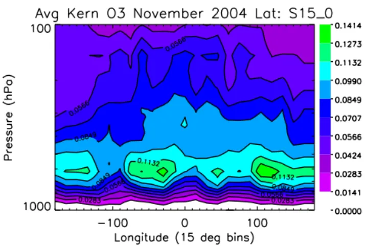
Fig. 1. Mean of the ozone averaging kernel diagonals for TES ob-servations from 15 S to the equator. The mean values are calculated in 15×15 degree bins.
cloud optical depth, as well as the retrieved state. For exam-ple, higher ozone concentrations result in greater sensitivity and therefore higher values in the averaging kernel. Figure 1 shows the average of the diagonal of the averaging kernel matrix from 15 S to the equator as a function of longitude for TES estimates of ozone for the 4–16 November time period. Larger values indicate greater sensitivity to the atmospheric state at their corresponding pressure levels. The peaks of the averaging kernel matrix are centered near 750 hPa indicat-ing that TES observations have significant sensitivity to the lower troposphere.
A suite of quality criteria are used for selection of the ob-servations. For ozone, the absolute radiance residual mean is less than 0.1, the radiance root mean square value is between 0.5 and 1.75, the retrieved cloud top pressure is between 90 and 1300 hPa, the absolute difference between surface tem-perature and atmospheric temtem-perature is less than 25 K, the absolute difference of the emissivity from its a priori value is less than 0.04, and the absolute difference between the sur-face temperature and its a priori value is less than 8 K (Oster-man, 2007).
2.3 Construction of the TES observation operator and comparison to chemistry and transport models
The vertical resolution and bias characterized by Eq. (3) must be taken into account in order to compare TES ozone and CO profile estimates with in-situ measurements and mod-eled profiles. The TES observation operator is constructed to perform this function and will be shown for comparison with a chemistry and transport model (CTM). A CTM can be described by a “forward” model
(a)
(b)
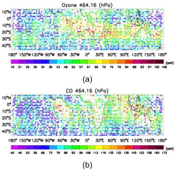
Fig. 2. (a)TES ozone estimates and(b)TES CO at 464.14 hPa from 4–16 November 2004 using V002 data.
wherexi,mt is the vector whose elements are the natural log-arithm of the vertical distribution of the model atmospheric state, e.g., CO, at locationiand timet,yt is a vector whose
elements are the 3-D distribution of the atmospheric state,ut
is a vector whose elements contain key source and sink terms for the atmospheric state, andF is the model operator that in-terpolates the global atmospheric state to the TES footprint at locationi. The TES observation operator is
Hit(xt,ut, t )=xit,a+Ait(x i,m
t −xit,a). (5)
The natural logarithm operation on the CTM model opera-tor in Eq. (4) accounts for the fact that TES retrievals of trace gases such as ozone and CO are performed on the natural log-arithm of those gases. By implication, the a priori state vector and averaging kernel matrix are also in natural logarithm and consequently the statistics are assumed to be lognormal in distribution. In the case where the actual atmospheric state is
equal to Eq. (4), then the TES profile estimate can be written in the standard noise model
ˆ
xi,mt =Hit(yt,ut, t )+ǫ. (6)
Equation (6) includes both the vertical resolution and charac-terized errors in the TES retrieval. Subtracting Eq. (5) from (1) results in
ˆ
(a)
>
(b)
>
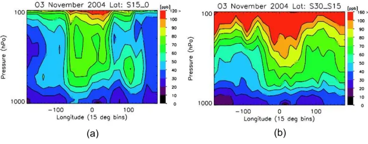
Fig. 3. Longitudinal distribution of TES ozone from(a)15 S-0(b)30 S–15 S averaged from 4–16 November 2004 in 15◦×15◦bins.
3 Overview of TES tropical tropospheric ozone and carbon monoxide observations
TES observations of ozone and CO are shown from 15 N to 30 S at 464 hPa from 4–16 November 2004 in Fig. 2. The most notable feature is a band of elevated ozone starting from Eastern Brazil through both the Atlantic and Indian Oceans and extending into the Pacific. The highest ozone concentrations are observed both over the tropical Atlantic (>100 ppbv) and over Madagascar. This pervasive zonal ozone distribution has been observed from satellites, in par-ticular from the total ozone mapping spectrometer (TOMS) using a tropospheric ozone residual technique (Fishman and Larsen, 1987; Fishman et al., 1991, 2003). This distribution is due in part to the recirculation of ozone and ozone pre-cursors between South America and sub-equatorial Africa over the Atlantic (Krishnamurti et al., 1996; Thompson et al., 1996; Sinha et al., 2004; Moxim and Levy, 2000; Martin et al., 2002; Sauvage et al., 2005; Jenkins and Ryu, 2004b; Chatfield et al., 2004; Edwards et al., 2003; Wang et al., 2006).
In addition, a high pressure system centered over Australia seen from the NCEP reanalysis (not shown, but available at http://www.cdc.noaa.gov/HistData/), low monthly averaged cloud optical depths from the International Satellite Cloud Climatology Project (ISCCP) (Rossow and Schiffer, 1991; Rossow et al., 1993) (available at http://isccp.giss.nasa.gov/), and relatively high biomass burning (van der Werf et al., 2006) indicate conditions favorable to ozone formation. TES observations of mid-tropospheric ozone show enhanced val-ues extending northwest of Australia into Indonesia, which have been associated with El Ni˜no conditions (Thompson et al., 2001; Chandra et al., 2007; Logan et al., 2008).
TES observations of CO show a plume from South Amer-ica extending eastward into the Western Pacific consistent with previous satellite and aircraft observations (Chatfield et al., 2002; Edwards et al., 2006). Similar to TES ozone, Indonesia-Australia region shows elevated concentrations of TES CO comparable to South America and sub-equatorial Africa. MODIS firecounts are elevated across Northern Australia and Eastern Africa (not shown but available at http://rapidfire.sci.gsfc.nasa.gov/firemaps/) are indicative of a continued presence of continental biomass burning emis-sion sources even as the Southern Hemisphere transitions to its Austral summer, wet season. In addition, the per-vasive high values of CO across the Indian ocean suggest the outflow of continental emissions, which are shown by CO tagged tracers for S. America, subequatorial Africa, and Indonesia/Australia in Jones et al. (2009) and are consis-tent with previous studies from the Southern African Fire-Atmosphere Research Initiative (SAFARI), e.g., (Garstang et al., 1996).
3.1 Comparison of TES ozone to the SHADOZ network
Fig. 4. SHADOZ ozone sonde measurements for November 2004. Location and the number of sondes used in the average are shown across the top of the figure. Most of the sites are between 0–15◦S.
total of 30 sondes were used in the average ranging from just one sonde measurement at Java to 6 sonde measurements at Natal. In the tropical Atlantic between 0 and 30 W, As-cencion (8 S, 14.4 W) and Natal (5.8 S, 35.2 W) show middle tropospheric values between 60–80 ppb, consistent with TES observations in Fig. 3. At the Java site (7.5 S, 112.6 E), el-evated ozone concentrations of 50–70 ppb are observed be-tween 700–400 hPa while TES observations over the same region indicate a similar enhancement. The vertical struc-ture of the ozone over Indonesia is somewhat different than ozone enhancements over the tropical Atlantic and Western Indian Ocean suggesting that different processes are control-ling ozone formation there.
The vertical distribution of TES ozone from 30 S to 15 S are shown in Fig. 3b. Elevated ozone stretches from South-ern Brazil across the Atlantic and Africa into most of the Indian Ocean. This elevated ozone is pervasive from roughly 500–200 hPa. Comparison between Pretoria (25.9 S, 28.2 E) and TES observations show similar values of ozone (80–100 ppb) between 400–200 hPa whereas Reunion Island (21.1 S, 55.5 E) indicates significantly higher ozone above
200 hPa. Similar to the ozone distribution in Fig. 2, higher amounts of ozone are seen throughout the troposphere over the Indian Ocean relative to the remote Pacific by roughly 10–20 ppb, consistent with transport of ozone from South America, South Atlantic, and Africa into the Indian Ocean.
4 Comparison of GEOS-Chem to TES estimates of CO and ozone
4.1 Description of GEOS-Chem
(a) (b)
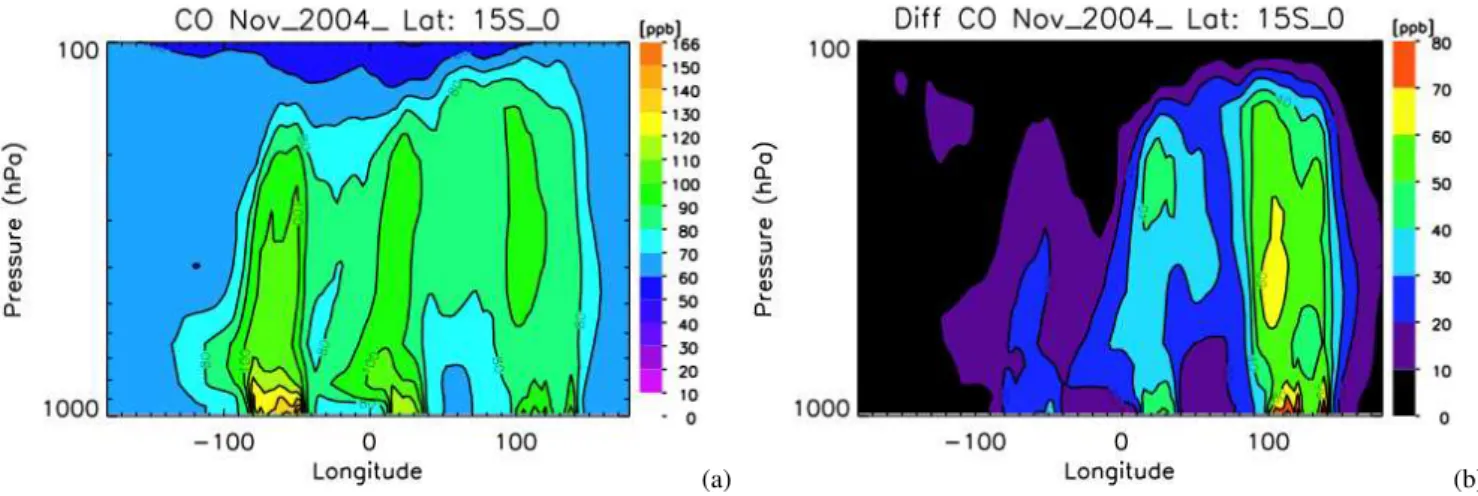
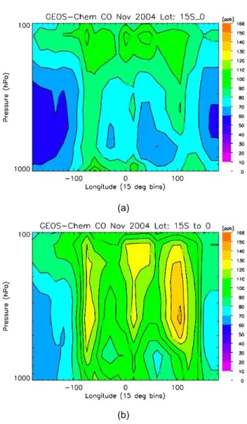
Fig. 5. (a)Zonal distribution of CO from GEOS-Chem from 15◦S-0. The data is averaged in 15◦×15◦bins in both longitude and latitude.
(b)Average difference in the GEOS-Chem zonal CO distribution between the a priori and a posteriori fields based on 15◦×15◦bins.
layers. Here we degrade the horizontal resolution to 2◦×2.5◦ from the surface up to 0.01 hPa. The model includes a complete description of tropospheric O3-NOx-hydrocarbon
chemistry, including sulfate aerosols, black carbon, organic carbon, sea salt, and dust. The lightning parameterization and magnitudes has been described by Martin et al. (2002) and used by (Hudman et al., 2007). For this study, global source of NOx from lightning was 4.7 TgN/a. The
limita-tions of the lightning parameterization in this version of the model are discussed in (Sauvage et al., 2007b). Anthro-pogenic emissions in the model are described in (Duncan et al., 2007). While these emissions are based on an ear-lier time period, their values are within the observed vari-ability and are roughly between more recent bottom-up and top-down emissions estimates (Bian et al., 2007). Extensive evaluations of the GEOS-Chem tropospheric ozone simula-tions have been conducted by (Wu et al., 2007; Martin et al., 2002; Liu et al., 2006).
4.2 Comparison of GEOS-Chem to TES CO over the southern tropics
The GEOS-Chem CO zonal distribution from 15◦S to the equator is shown in Fig. 5a. The results are averaged from 4–16 November 2004 in 15◦×15◦bins. This simulation used climatological biomass burning emissions, which result in el-evated values of CO over South America, Africa, and Indone-sia/Australia. In the lower and middle troposphere, CO over South America dominates the region with values up to 40 ppb higher than Indonesia/Australia. The zonal distribution of TES CO from 15◦S-0 is shown in Fig. 6. These retrievals also are averaged in 15◦longitudinal bins with roughly 20– 30 observations per bin. For comparison, the GEOS-Chem CO fields were sampled at the coincident TES observation coordinates and the TES observation operator, (Eq. 5), was applied as shown in Fig. 7a. There is significant disagree-ment both in the magnitude and relative distribution of the
Fig. 6. Zonal distribution of TES CO estimates from 15 S to the equator. The data is averaged in 15 degree bins in both longitude and latitude.
GEOS-Chem and TES CO observations with differences up to 40 ppb. TES observations in Fig. 6 show that CO over Indonesia/Australia was as high as that over South America. TES and MOPITT CO observations were used to estimate the CO source emissions over the globe in (Jones et al., 2009). The a priori and a posteriori emissions for South America, sub-equatorial Africa, and Australia/Indonesia are listed in Table 1. For this time period, the emissions were es-timated to be over twice as high as those in the a priori sim-ulation. The GEOS-Chem results at the TES resolution and sampling with the a posteriori emission are shown in Fig. 7b. The a posteriori CO distribution from GEOS-Chem between 15◦S and the equator is in remarkably good agreement with the TES observations shown in Fig. 6.
(a)
(b)
Fig. 7. (a)Zonal distribution of CO from GEOS-Chem sampled over the same observations as TES. For each observation point, the TES observation operator is applied to the GEOS-Chem fields. The resulting fields are averaged in 15 degree bins in both longitude and latitude. (b)Zonal CO distribution from the equator to 15 S from GEOS-Chem evaluated with a posteriori emissions and TES observation operator.
or 85% near the surface and approximately 60 ppb or a 65% increase throughout the free troposphere. Over the Indian Ocean, the CO distribution in GEOS-Chem increased by about 35 ppb and around 45 ppb over sub-equatorial Africa in the 200–400 hPa region. Over South America, the increase is modest – no more than 30 ppb.
4.3 Observations of lightning and surface NOx
The concentrations and distribution of NOx has a
signifi-cant impact of the distribution of ozone (Jacob et al., 1996). In the Southern Hemisphere, the primary sources of surface
Table 1. A priori and a posteriori emissions taken from (Jones et al., 2009).
Region a priori (Tg CO/y) a posteriori
S. America 113 118
S. Africa 95 173
Indonesia/Ausralia 69 155
NOxare biomass burning, fossil fuel and biofuel combustion
(Jaegl´e et al., 2005). These emissions can produce ozone near the surface which can in turn be convectively lofted into the upper troposphere (Chatfield and Delany, 1990). How-ever, NOx from lightning is directly emitted into the
up-per troposphere and can play a dominant role in the pro-duction of tropical ozone downwind (Pickering et al., 1998; Sauvage et al., 2007a; Martin et al., 2007; Boersma et al., 2005; Moxim and Levy, 2000).
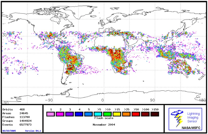
The Lightning Imaging Sensor (LIS) aboard the Tropi-cal Rainfall Measuring Mission (TRMM) estimates lightning flash counts by means of a high speed CCD imaging sen-sor (3–6 km horizontal resolution) in conjunction with a nar-row band (λ=777 nm) filter. Lightning flash counts from LIS are shown in Fig. 8 for November 2004. For this month, lightning flash counts are densely distributed over North-ern Argentina and to a lesser extent SoutheastNorth-ern Brazil, throughout tropical Africa and Southern Africa with rates ex-ceeding 150. By comparison, Indonesia/Northern Australia shows markedly less flash counts with rates generally less than 25. This distribution is consistent a the high pressure system from NCEP reanalysis and low ISCCP cloud opti-cal depth centered over Indonesia (not shown but available at http://www.cdc.noaa.gov/ and http://isccp.giss.nasa.gov/). We further investigated the influence of lightning on the a posteriori ozone distribution in GEOS-Chem by comparing against a separate run with lightning turned off as shown in Fig. 9. The spatial distribution of the ozone difference over the Indonesia/Australian region is significantly less than over sub-equatorial Africa and S. America at 7.8 km. Conse-quently, we could expect the regional contribution of ozone from lightning NOxover Indonesia/Australia to be less than
the regional contribution of lightning to South America and Africa.
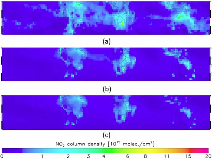
The distribution of lower tropospheric NO2can be
investi-gated from monthly averaged tropospheric NO2columns
de-rived from the Ozone Monitoring Instrument (OMI), (Lev-elt et al., 2006), which are shown in Fig. 10a for 1–14 November 2004. The columns are calculated using the the retrieval-assimilation algorithm described in (Boersma et al., 2004, 2007). Individual OMI tropospheric NO2
observa-tions with approximate horizontal resoluobserva-tions of 25×24 km2 have been gridded onto a 0.5◦×0.5◦grid. To avoid situations with clouds screening the NO2underneath, only cloud-free
Fig. 8. Observations of lightning flash counts from the Lightning Imaging Sensor (LIS) for November 2004.
The estimated uncertainty for individual OMI observations is on the order of 30–50% for situations with appreciable NO2
columns (>1 1015molec cm2), but it is anticipated that the averaging of large numbers of pixels here reduces the uncer-tainty of the monthly average to within 5–10%. Given these uncertainties, NO2tropospheric column values on the order
of 4 1015molec cm2are concentrated south of the mouths of the Amazon in Brazil as well as Northern Australia. With the exception of the Johannesburg region in South Africa where values approach 8 1015molec cm2, tropospheric NO2
are roughly 2 1015molec cm2in sub-equatorial Africa. The assumption that NOx sources scale with CO was
tested by comparing GEOS-Chem a posteriori and a priori NO2 columns to OMI NO2 as shown in Fig. 10b, c. The
spatial distribution of GEOS-Chem generally agrees with OMI but does not capture the enhance NO2 concentrations
in Northern Australia, which are consistent with the concen-trated MODIS firecounts. The a posteriori derived NO2are in
better agreement than the a priori with observations but still generally underestimate the NO2 columns. There are
sev-eral possible explanations for this discrepancy. OMI obser-vations are more sensitive to surface concentrations whereas TES/MOPITT are more sensitive to the free troposphere. Errors in convection and boundary layer transport within
GEOS-Chem could lead to an underestimate of the bound-ary flux of trace gases into the free troposphere. However, Jones et al. (2009) showed that the a posteriori emissions reduced the bias in the modelled CO with respect to GMD surface data at Guam. On the other hand, the relative contri-bution of NO2and CO to increasing emissions is assumed to
be known. Given that the inverse estimate did not distinguish between types of sources, e.g., biofuels or biomass burning, we could expect that the NO2fields may not scale uniformly.
Nevertheless, in the absence of additional information on the different source types and solving simultaneously for NOx
and CO emissions, uniformly scaling the emissions is a rea-sonable approach.
4.4 Comparison of GEOS-Chem to TES and SHADOZ ozone over the southern tropics
Fig. 9. Difference between the GEOS-Chem ozone distribution with a posteriori emissions without and with lightning at 7.8 km.
Pacific. This enhancement is also observed in Fig. 12a where the TES observation operator has been applied to the GEOS-Chem fields. In both cases, the ozone amounts are less than those observed by TES in Fig. 3 over both the tropical At-lantic and Indonesia/Australia.
The ozone distribution from GEOS-Chem was also cal-culated based on the revised emissions where all emissions, including NOx and hydrocarbons (but not aerosols), were
scaled with the CO a posteriori emission estimates. The GEOS-Chem fields with the a posteriori emissions sampled along the TES observations are shown in Fig. 12b. There is a significant increase in upper tropospheric ozone at 200 hPa of about 8–10 ppb on the Eastern coast of Africa near 40 E. In addition, an overall increase of about 10 ppb throughout the troposphere can be seen over Indonesia/Australia. Use of the a posteriori emissions improves agreement between the model and TES ozone, but significant discrepancies remain over the Atlantic, eastern sub-equatorial Africa, and Indone-sia.
The difference between the TES observations of ozone and GEOS-Chem with a priori (top panels) and a posteriori (bot-tom panels) emissions are shown in Fig. 13 for 15 S to the equator and Fig. 14 for 30 S to 15 S. The top panels show the largest differences in ozone are centered over the Atlantic and Indonesia. With the a posteriori emissions, the bottom panels show an overall decrease in ozone differences that is fairly uniform zonally. Over the tropical Atlantic, the difference between GEOS-Chem and TES are reduced by roughly 5 ppb from 30 S-0. The reduction over the Indonesia/Australia re-gion in the mid-troposphere is more substantial: up to 10 ppb.
On the other hand, the upper tropospheric ozone differences at 100 E and 100 W from 15 S-0 increased with the a posteri-ori emissions. With those exceptions, TES observations are higher everywhere relative to GEOS-Chem.
Comparisons can also be made between GEOS-Chem with the SHADOZ sondes over the same time period as shown in Fig. 15 for four representative states in the tropical At-lantic, South Africa, Reunion, and Indonesia. The number of observations per site vary from one to three, which does not permit a statistical comparison. However, they do al-low for an analysis the surface emission response at finer vertical scales. Over the Ascension Islands, the free tro-pospheric ozone response is relatively small consistent with the modest change in emissions from South America, which is shown by the tagged tracer calculations in (Jones et al., 2009). The absolute difference between GEOS-Chem and the ozone sondes is significant, over 50 ppb in the upper tro-posphere. Over the Atlantic, the residual differences and their spatial structure could be attributed in part to ozone generated from lightning NOx. In (Sauvage et al., 2007a),
in-creasing the intra-cloud to ground-to-cloud flash ratio to 0.75 for lightning NOx formation considerably improved
Fig. 10. (a)OMI(b)GEOS-Chem a posteriori(c)GEOS-Chem a priori NO2tropospheric columns for 1–14 November 2004 from the equator to 40 S.
The response of ozone to the surface emissions is greater in the lower troposphere than in the upper troposphere over Pretoria. The lower tropospheric ozone distribution is in bet-ter agreement with the ozone sonde measurement indicating that the lower tropospheric ozone is significantly influenced by surface emissions. On the other hand, the predicted up-per tropospheric ozone in Reunion and Pretoria substantially underestimates ozone relative to the sonde measurements. While this analysis can not address cause, this discrepancy could be due to outflow of ozone from lightning-generated NOxor stratospheric intrusions.
For the Java site in Fig. 15b, both the boundary layer and free troposphere is sensitive to surface emission changes in the model. Consistent with the TES observations, the Java site shows elevated lower tropospheric ozone concentra-tions between 50–70 ppb. The satellite-constrained a posteri-ori emissions result in better ozone agreement in the lower troposphere between the model and the sonde measure-ment. This agreement between satellite-constrained emis-sions, TES ozone, and SHADOZ ozone provides strong
ev-idence that the ozone enhancements are in fact due to local sources. However, GEOS-Chem does not represent the low ozone between 300–150 hPa. This low ozone is probably due to the mixing of ozone-poor marine air over Java. Dynamical and chemical changes across coastal regions represent sub-grid scale processes at the GEOS-Chem resolution. There-fore, we could expect the model to have difficulty in captur-ing the vertical distribution of ozone when it is influenced by these processes.
4.5 Response of the free troposphere in GEOS-Chem to surface emissions
(a)
(b)
>
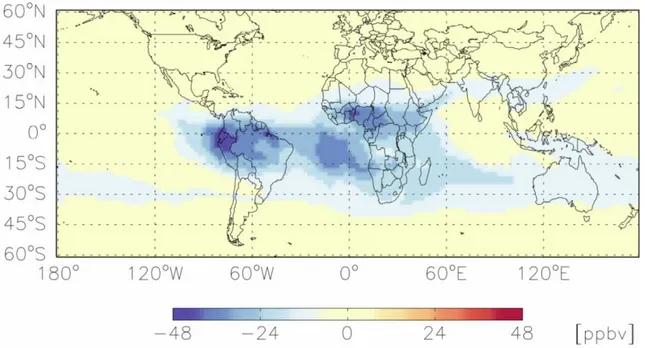
Fig. 11. (a)Zonal distribution of ozone from GEOS-Chem aver-aged in 15◦bins in longitude and latitude from the equator to 15◦S.
(b)Average difference in GEOS-Chem ozone fields between a pri-ori and a posteripri-ori emissions based on 15◦×15◦bins.
by up to 16 ppb in the upper troposphere centered around 150 hPa. It is in this upper tropospheric region, as shown in Fig. 13b, that GEOS-Chem ozone is greater than the TES ob-servations by up to 15%. The ozone response to the emission changes over sub-equatorial Africa is approximately 8 ppb near the surface and around 200 hPa. Over South Amer-ica, there were few changes in the ozone distribution, consis-tent with a modest increase in emission strengths. Curiously, there was a significant increase in ozone in the remote Pacific centered around 150 W in the upper troposphere (>15%).
The principal chemical mechanism for the ozone response in the free troposphere to changes in surface emissions is the ambient NOxdistribution. CO is assumed to be a tracer
of combustion emissions generally and consequently all the combustion emissions, including NOx, are scaled along with
the CO emissions derived from the inverse analysis.
How-(a)
>
(b)
>
Fig. 12. (a)Zonal distribution of ozone from GEOS-Chem with the TES observation operator applied averaged from 15◦S to the equator. The distribution is calculated from averaged 15◦bins in longitude and latitude. (b)GEOS-Chem ozone fields with a pos-teriori emissions from the equator to 15◦S sampled along the TES orbit and vertical resolution. The data is averaged in 15◦×15◦bins.
ever, the NOxzonal distribution has a different response to
the scaled emissions than the CO distribution. The NOx
dis-tribution based on the GEOS-Chem a priori emissions and the change in mean zonal NOx from the a posteriori
emis-sions are shown in Fig. 16. The a priori NOxfields are
high-est over South America where the values are up to 6–7 times higher than over Indonesia/Australia and up to twice as high as sub-equatorial Africa. Previous research indicate that con-centrations of NOxin the free troposphere are due primarily
to lightning sources (Pickering et al., 1998; Folkins et al., 2006), with the South American and sub-equatorial African regions exhibiting a much larger source of NOxfrom
(a)
(b)
Fig. 13. (a) Mean difference between(a)TES ozone observations and GEOS-Chem with a priori emissions and(b) TES ozone ob-servations and GEOS-Chem with a posteriori emissions and from 15 S to the equator. Mean differences are calculated between the TES observations and model predictions sampled along orbit track within 15◦×15◦bins.
Associated with these higher concentrations of NOx, model
simulations produce more ozone (Fig. 11) over South Amer-ica and sub-equatorial AfrAmer-ica than over Indonesia/Australia. The low ozone abundance in the upper troposphere over In-donesia/Australia as shown in Fig. 15b, however, also reflects convective transport of ozone-poor marine air to the upper troposphere (Lelieveld et al., 2001).
The greatest increase in free tropospheric NOx (50 ppt)
to the a posteriori emissions is centered over the Java Sea (115 E) at 150 hPa just to the East of the high NOx
concen-trations over Sumatra (105 E). Conversely the greatest de-crease (>120 ppt) in free tropospheric NOxis located over
the western coast of Africa. In addition, there is a significant decrease over South America (>55 ppt) centered at 250 hPa. The response of free tropospheric NOx to increases in the
(a)
(b)
Fig. 14. Mean difference between(a)TES ozone observations and GEOS-Chem with a priori emissions and(b)TES ozone observa-tions and GEOS-Chem with a posteriori emissions and from 30 S to 15 S. Mean differences are calculated between the TES observations and model predictions sampled along orbit track within 15◦×15◦ bins.
surface emissions, which include surface NOx, is a
non-linear function of both the ambient amounts of ozone, NOx,
and OH along with the chemical composition of lofted emis-sions (Kunhikrishnan and Lawrence, 2004; Liu et al., 1987). Figure 17 shows the response of peroxyacetylnitrate (PAN), which is an important sink and source for NOx, to surface
emission changes from GEOS-Chem. PAN increases over all three continents but is most significant over sub-equatorial Africa (>150 ppt at 200 hPa) and Indonesia (≈200 ppt at 600 hPa). Clearly, there is a significantly different response in GEOS-Chem over Indonesia where ozone, CO, NOx, and
(a)
(b)
(c)
(d)
Fig. 15. Comparison of GEOS-Chem ozone fields evaluated at a priori (red) and a posteriori (green) emissions with averaged SHADOZ sondes at(a)Ascension Island(b)Java(c)Pretoria(d)Reunion Island. The coordinates and number of observations used in the average are indicated in the titles.
A potentially important difference between the three trop-ical continental regions is the distribution of organics such as acetaldehyde, acetone, and formaldehyde in the free tropo-sphere. Acetaldehyde, for example, is oxidized by reaction with OH to produce peroxyacetyl radicals (CH3C(O)OO)
that in turn react with NO2to form PAN. In the GEOS-Chem
simulations, the response of these acetaldehyde (not shown) are up to three times larger over sub-equatorial African rel-ative to Indonesia. These chemical responses suggest that in GEOS-Chem differences in organics from lofted surface emissions over South America and sub-equatorial Africa preferentially lead to the formation of PAN at the expense of NOx and consequently mute the production of ozone.
On the other hand, increased surface emissions in
Indone-sia/Australia, while leading to enhanced PAN, do not lead to a reduction of NOx due to the overall lower background
concentrations of NOx, OH, and carbonyl compounds.
(a)
(b)
Fig. 16. (a)Zonal NOxconcentrations in GEOS-Chem based on
a priori emissions. (b)Mean difference in the zonal NOx
distri-bution between a priori and a posteriori surface emission estimates between 15 S and the equator during 4–16 November 2004. Data is averaged over 15◦×15◦bins.
5 Conclusions
We have investigated the impact of surface emissions on the zonal structure of tropical tropospheric ozone with a focus on the sensitivity of that distribution to changes in surface emis-sions between South America, sub-equatorial Africa, and In-donesia/Australia for November 2004.
Against the backdrop of the “wave-one” pattern of ele-vated ozone in the tropical Atlantic, TES ozone profiles also indicate enhanced values over Indonesia/Australia with vol-ume mixing ratios up to 70 ppb at 600 hPa. This enhance-ment is consistent with a SHADOZ sonde observation over Java. Co-located CO profiles from TES and NO2 columns
from OMI indicate concentrations over Indonesia/Australia are comparable to those over South America and Africa.
(a)
(b)
Fig. 17. (a)Zonal PAN distribution from GEOS-Chem.(b)Mean difference in the zonal PAN distribution between a priori and a pos-teriori surface emission estimates between 15 S and the equator dur-ing 4–16 November 2004. Data is averaged over 15◦×15◦bins.
From this observational context, we assessed the contri-bution of surface emissions to tropical ozone using GEOS-Chem simulations with a posteriori emissions derived from a linear inverse model, which was based on TES and MO-PITT CO (Jones et al., 2009). Based on over a factor of 2 increase in surface emissions in sub-equatorial Africa and Indonesia/Australia, the overall difference between TES and GEOS-Chem ozone was reduced throughout the troposphere between 30 S-0. Over Africa and Indonesia/Australia the discrepancies between GEOS-Chem and TES decreased by roughly 10 ppb.
The residual differences in ozone of 10–20 ppb in the mid-troposphere over the tropical Atlantic are consistent with the differences found in (Sauvage et al., 2007a) associated with underestimates of lightning NOxformation in
GEOS-Chem for the September-October-November season. In ad-dition, there is a residual difference over Indonesia/Australia at 600 hPa of up to 15 ppb that can not be explained by scal-ing the surface emissions.
We investigated these residual differences further by ex-amining the spatial patterns in GEOS-Chem estimates of ozone, CO, NOx, and PAN from changes between the
a priori and a posteriori surface emissions. The great-est change to the free tropospheric ozone distribution from 15 S-0 was over Indonesia (<16 ppb) at 175 hPa, consistent with maximum positive changes in NOx(<100 ppt) and CO
(<70 ppb). Consequently, free tropospheric ozone over In-donesia/Australia is sensitive to changes in regional surface emissions and these emissions make a significant contribu-tion to the regional ozone budget.
On the other hand, the free tropospheric NOxdistribution
declined over Africa and South America with losses exceed-ing 150 ppt. We examined the PAN response as a possible loss mechanism for the NOx. Maximum increases in PAN,
which reached over 150 ppt, corresponded to the maximum decreases in the NOxdistribution. Therefore, conversion of
NOxto PAN can partially explain the decreases in NOxin
re-sponse to increases in surface emission over South America and Africa. If this mechanism is correct, then the sensitivity of the tropical Atlantic ozone to changes in surface emissions of NOx is low because of the large ambient distribution of
ozone and NOxfrom lightning. However, the enhanced PAN
could lead to additional ozone formation downwind through conversion of PAN back to NOx(Staudt et al., 2003). Given
the relatively short time frame for the study, this analysis should be extended to seasonal and yearly time periods to see if these mechanisms are robust over longer time scales. In addition, the use of adjoints will allow for a more sophis-ticated sensitivity analysis and provide the basis for chemi-cally consistent estimates of both emissions and ozone pro-duction (Henze et al., 2007; Sandu et al., 2005; Chai et al., 2007).
Based on scenarios discussed in the IPCC-4, the tropical latitudes are particularly sensitive to climate change in terms of precipitation and land-use (Solomon et al., 2007). Based on our results, the emissions from Indonesia/Australian are an important contributor to the zonal tropical ozone distribu-tion both in terms of the ozone produced and in the sensitiv-ity of ozone to changes in those emissions. Given the com-plex feedbacks between land-use, biomass burning, biofuel production, plant productivity, and CO2 uptake and
emis-sion, (Levine, 1999; Sitch et al., 2007; Lohman et al., 2007; Forster et al., 2007), quantifying the present and future im-pact of surface emissions to tropical ozone will be critical for understanding chemistry-climate coupling.
Acknowledgements. This work was performed, in part, at the Jet Propulsion Laboratory, California Institute of Technology, under a contract with the National Aeronautics and Space Administration (NASA). JAL was funded by a grant from NASA to Harvard University. DBJ was supported by funding from the Natural Sciences and Engineering Research Council of Canada. We also thank the SHADOZ program for making the sonde data accessible.
Edited by: J. Rinne
References
Arellano, A. F., Kasibhatla, P. S., Giglio, L., van der Werf, G. R., Randerson, J. T., and Collatz, G. J.: Time-dependent inversion estimates of global biomass-burning CO emis-sions using Measurement of Pollution in the Troposphere (MOPITT) measurements, J. Geophys. Res., 111, D09303, doi:10.1029/2005JD006613, 2006.
Beer, R. and Glavich, T.: Remote Sensing of the Troposphere by Infrared Emissions Spectroscopy, Appl. Optics, 1129, 42–51, 1989.
Bey, I., Jacob, D. J., Yantosca, R. M., Logan, J. A., Field, B. D., Fiore, A. M., Li, Q., Liu, H. Y., Mickley, L. J., and Schultz, M. G.: Global modeling of tropospheric chemistry with assim-ilated meteorology: Model description and evaluation, J. Geo-phys. Res., 106(D19), 23073–23095, 2001.
Bian, H., Chin, M., Kawa, S. R., Duncan, B., Arellano, A., and Kasibhatla, P.: Sensitivity of global CO simulations to uncertain-ties in biomass burning sources, J. Geophys. Res., 112, D23308, doi:10.1029/2006JD008376, 2007.
Boersma, K. F., Eskes, H. J., Veefkind, J. P., Brinksma, E. J., van der A, R. J., Sneep, M., van den Oord, G. H. J., Levelt, P. F., Stammes, P., Gleason, J. F., and Bucsela, E. J.: Near-real time retrieval of tropospheric NO2from OMI, Atmos. Chem. Phys.,
7, 2103–2118, 2007,
http://www.atmos-chem-phys.net/7/2103/2007/.
Boersma, K. F., Eskes, H. J., and Brinksma, E. J.: Error analysis for tropospheric NO2retrieval from space, J. Geophys. Res.-Atmos.,
109, D04311, doi:10.1029/2003JD003962, 2004.
Boersma, K. F., Eskes, H. J., Meijer, E. W., and Kelder, H. M.: Estimates of lightning NOxproduction from GOME satellite
ob-servations, Atmos. Chem. Phys., 5, 2311–2331, 2005, http://www.atmos-chem-phys.net/5/2311/2005/.
Bowman, K., Worden, J., Steck, T., Worden, H., Clough, S., and Rodgers, C.: Capturing time and vertical variability of tropo-spheric ozone: A study using TES nadir retrievals, J. Geophys. Res., 107(D23), 4723, doi:10.1029/2002JD002150, 2002. Bowman, K. W., Rodgers, C. D., Kulawik, S. S., Worden, J.,
Sarkissian, E., Osterman, G., Steck, T., Lou, M., Eldering, A., Shephard, M., Worden, H., Lampel, M., Clough, S., Brown, P., Rinsland, C., Gunson, M., and Beer, R.: Tropospheric Emis-sion Spectrometer: Retrieval Method and Error Analysis, IEEE T. Geosci. Remote, 44(5), 1297–1307, doi:10.1109/TGRS.2006. 871234, 2006.
Transformation Ozone Measurements, J. Geophys. Res.-Atmos., 112, D12S15, doi:10.1029/2006JD007763, 2007.
Chandra, S., Ziemke, J. R., Schoeberl, M. R., Froidevaux, L., Read, W. G., Levelt, P. F., and Bhartia, P. K.: Effects of the 2004 El Ni˜no on tropospheric ozone and water vapor, Geophys. Res. Lett., 34, L06802, doi:doi:10.1029/2006GL028779, 2007. Chatfield, R. B. and Delany, A.: Convection links biomass burning
to increased tropical ozone: However, models will tend to over-predict O3, J. Geophys. Res.-Atmos., 95, 18473–18488, 1990. Chatfield, R. B., Guo, Z., Sachse, G. W., Blake, D. R., and Blake,
N. J.: The subtropical global plume in the Pacific Exploratory Mission-Tropics A (PEM-Tropics A), PEM-Tropics B, and the Global Atmospheric Sampling Program (GASP): How tropical emissions affect the remote Pacific, J. Geophys. Res., 107(D16), 4278, doi:10.1029/2001JD000497, 2002.
Chatfield, R. B., Guan, H., Thompson, A. M., and Witte, J. C.: Con-vective lofting links Indian Ocean air pollution to paradoxical South Atlantic ozone maxima, Geophys. Res. Lett., 31, L06103, doi:10.1029/2001JD000497, 2004.
Duncan, B. N., Bey, I., Chin, M., Mickley, L. J., Fairlie, T. D., Martin, R. V., and Matsueda, H.: Indonesian wildfires of 1997: Impact on tropospheric chemistry, J. Geophys. Res., 108(D15), 4458, doi:10.1029/2002JD003195, 2003a.
Duncan, B. N., Martin, R. V., Staudt, A. C., Yevich, R., and Logan, J. A.: Interannual and seasonal variability of biomass burning emissions constrained by satellite observations, J. Geophys. Res., 108, 4100, doi:10.1029/2002JD002378, 2003b.
Duncan, B. N., Logan, J. A., Bey, I., Megretskaia, I. A., Yan-tosca, R. M., Novelli, P. C., Jones, N. B., and Rinsland, C. P.: Global budget of CO, 1988–1997: Source estimates and val-idation with a global model, J. Geophys. Res., 112, D22301, doi:10.1029/2007JD008459, 2007.
Edwards, D. P., Lamarque, J.-F., Attie, J.-L., Emmons, L. K., Richter, A., Cammas, J.-P., Gille, J. C., Francis, G. L., Deeter, M. N., Warner, J., Ziskin, D. C., Lyjak, L. V., Drummond, J. R., and Burrows, J. P.: Tropospheric ozone over the tropical At-lantic: A satellite perspective, J. Geophys. Res., 108(D8), 4237, doi:10.1029/2002JD002927, 2003.
Edwards, D. P., Emmons, L. K., Gille, J. C., Chu, A., Atti´e, J.-L., Giglio, L., Wood, S. W., Haywood, J., Deeter, M. N., Massie, S. T., Ziskin, D. C., and Drummond, J. R.: Satellite-observed pollution from Southern Hemisphere biomass burning, J. Geo-phys. Res.-Atmos., 111, D14312, doi:10.1029/2005JD006655, 2006.
Fishman, J. and Larsen, J. C.: Distribution of total ozone and strato-spheric ozone in the tropics: Implications for the distribution of tropospheric ozone, J. Geophys. Res., 92, 6627–6634, 1987. Fishman, J., Ramanathan, V., Crutzen, P. J., and Liu, S. C.:
Tropo-spheric ozone and climate, Nature, 282, 818–820, doi:10.1038/ 282818a0, 1979.
Fishman, J., Fakhruzzaman, K., Cros, B., and Nganga, D.: Iden-tification of Widespread Pollution in the Southern Hemisphere deduced from satelite analyses, Science, 252, 1693–1696, 1991. Fishman, J., Wozniak, A. E., and Creilson, J. K.: Global distribution of tropospheric ozone from satellite measurements using the em-pirically corrected tropospheric ozone residual technique: Iden-tification of the regional aspects of air pollution, Atmos. Chem. Phys., 3, 893–907, 2003,
http://www.atmos-chem-phys.net/3/893/2003/.
Folkins, I., Bernath, P., Boone, C., Donner, L. J., Eldering, A., Lesins, G., Martin, R. V., Sinnhuber, B.-M., and Walker, K.: Testing convective parameterizations with tropical measure-ments of HNO3, CO, H2O, and O3: Implications for the
wa-ter vapor budget, J. Geophys. Res.-Atmos., 111, D23304, doi: doi:10.1029/2006JD007325, 2006.
Forster, P., Ramaswamy, V., Artaxo, P., Berntsen, T., Betts, R., Fa-hey, D., Haywood, J., Lean, J., Lowe, D., Myhre, G., Nganga, J., Prinn, R., Raga, G., Schulz, M., and Dorland, R. V.: Cli-mate Change 2007: The Physical Science Basis, Contribution of Working Group I to the Fourth Assessment Report of the Inter-governmental Panel on Climate Change, chap. Changes in Atmo-spheric Constituents and in Radiative Forcing, Cambridge Uni-versity Press, 131–217, 2007.
Garstang, M., Tyson, P. D., Swap, R., Edwards, M., Kallberg, P., and Lindesay, J. A.: Horizontal and vertical transport of air over southern Africa, J. Geophys. Res.-Atmos., 101, 23721–23736, 1996.
Hauglustaine, D., Emmons, L., Newchurch, M., Brasseur, G., Takao, T., Matsubara, K., Johnson, J., Ridley, B., Stith, J., and Dye, J.: On the Role of Lightning NOxin the Formation of
Tro-pospheric Ozone Plumes: A Global Model Perspective, J. At-mos. Chem., 38, 277–294, 2001.
Henze, D. K., Hakami, A., and Seinfeld, J. H.: Development of the adjoint of GEOS-Chem, Atmos. Chem. Phys., 7, 2413–2433, 2007, http://www.atmos-chem-phys.net/7/2413/2007/.
Horowitz, L.: Past, present, and future concentrations of tropo-spheric ozone and aerosols: Methodology, ozone evaluation, and sensitivity to aerosol wet removal, J. Geophys. Res.-Atmos., 111, D22211, doi:10.1029/2005JD006937, 2006.
Hudman, R. C., Jacob, D. J., Turquety, S., Leibensperger, E. M., Murray, L. T., Wu, S., Gilliland, A. B., Avery, M., Bertram, T. H., Brune, W., Cohen, R. C., Dibb, J. E., Flocke, F. M., Fried, A., Holloway, J., Neuman, J. A., Orville, R., Perring, A., Ren, X., Sachse, G. W., Singh, H. B., Swanson, A., and Wooldridge, P. J.: Surface and lightning sources of nitrogen oxides over the United States: Magnitudes, chemical evolution, and outflow, J. Geo-phys. Res., 112, D12S05, doi:10.1029/2006JD007912, 2007. Jacob, D., Heikes, B. G., Fan, S.-M., Logan, J. A., Mauzerall, D. L.,
Bradshaw, J. D., Singh, H. B., Gregory, G. L., Talbot, R. W., Blake, D. R., and Sachse, G. W.: Origin of ozone and NOxin the
tropical troposphere: A photochemical analysis of aircraft obser-vations over the South Atlantic basin, J. Geophys. Res.-Atmos., 101, 24235–24250, doi:10.1029/96JD00336, 1996.
Jacob, D. J.: Introduction to Atmospheric Chemistry, Princeton University Press, New Jersey, 1999.
Jaegl´e, L., Steinberger, L., Martin, R. V., and Chance, K.: Global partitioning of NOxsources using satellite observations: Relative
roles of fossil fuel combustion, biomass burning and soil emis-sions, Faraday Discuss., 130, 407–423, doi:10.1039/b502128f, 2005.
Jenkins, G. S. and Ryu, J.-H.: Space-borne observations link the tropical atlantic ozone maximum and paradox to lightning, At-mos. Chem. Phys., 4, 361–375, 2004a.
Jones, D. B. A., Bowman, K. W., Palmer, P. I., Worden, J. R., Jacob, D. J., Hoffman, R. N., Bey, I., and Yantosca, R. M.: Potential of observations from the Tropospheric Emission Spectrometer to constrain continental sources of carbon monoxide, J. Geophys. Res.-Atmos., 108, 4789, doi:doi:10.1029/2003JD003702, 2003. Jones, D. B. A., Bowman, K. W., Logan, J. A., Heald, C. L., Liu, J.,
Luo, M., Worden, J., and Drummond, J.: The zonal structure of tropical O3and CO as observed by the Tropospheric Emission Spectrometer in November 2004 – Part 1: Inverse modeling of CO emissions, Atmos. Chem. Phys., 9, 3547–3562, 2009, http://www.atmos-chem-phys.net/9/3547/2009/.
Jourdain, L., Worden, H. M., Worden, J. R., Bowman, K., Li, Q., El-dering, A., Kulawik, S. S., Osterman, G., Boersma, K. F., Fisher, B., Rinsland, C. P., Beer, R., and Gunson, M.: Tropospheric ver-tical distribution of tropical Atlantic ozone observed by TES dur-ing the northern African biomass burndur-ing season, Geophys. Res. Lett., 34, L04810, doi:10.1029/2006GL028284, 2007.
Kiehl, J. T., Schneider, T. L., Portmann, R. W., and Solomon, S.: Climate forcing due to tropospheric and stratospheric ozone, J. Geophys. Res.-Atmos., 104, 31239–31254, 1999.
Krishnamurti, T., Sinha, M. C., Kanamitsu, M., Oosterhof, D., Fuel-berg, H., Chatfield, R., Jacob, D. J., and Logan, J.: Passive tracer transport relevant to the TRACE A experiment, J. Geophys. Res., 101, 23889–23908, doi:10.1029/95JD02419, 1996.
Kunhikrishnan, T. and Lawrence, M. G.: Sensitivity of NOxover
the Indian Ocean to emissions from the surrounding continents and nonlinearities in atmospheric chemistry responses, J. Geo-phys. Res., 31, L15109, doi:10.1029/2004GL020210, 2004. Lacis, A., Wuebbles, D. J., and Logan, J. A.: Radiative forcing of
climate by changes in the vertical distribution of ozone, J. Geo-phys. Res., 95, 9971–9981, doi:10.1029/90JD00092, 1990. Lelieveld, J., Crutzen, P. J., Ramanathan, V., Andreae, M. O.,
Bren-ninkmeijer, C. A. M., Campos, T., Cass, G. R., Dickerson, R. R., Fischer, H., de Gouw, J. A., Hansel, A., Jefferson, A., Kley, D., de Laat, A. T. J., Lal, S., Lawrence, M. G., Lobert, J. M., Mayol-Bracero, O. L., Mitra, A. P., Novakov, T., Oltmans, S. J., Prather, K. A., Reiner, T., Rodhe, H., Scheeren, H. A., Sikka, D., and Williams, J.: The Indian Ocean Experiment: Widespread Air Pollution from South and Southeast Asia, Science, 291, 1031– 1036, doi:10.1126/science.1057103, 2001.
Levelt, P. F., van den Oord, G. H. J., Dobber, M. R., M¨alkki, A., Visser, H., de Vries, J., Stammes, P., Lundell, J. O. V., and Saari, H.: The Ozone Monitoring Instrument, IEEE T. Geosci. Remote, 44, 1093–1101, 2006.
Levine, J. S.: The 1997 fires in Kalimantan and Sumatra, Indonesia: Gaseous and particulate emissions, Geophys. Res. Lett., 26(7), 815–818, doi:10.1029/1999GL900067, 1999.
Li, Q., Jacob, D. J., Bey, I., Palmer, P. I., Duncan, B. N., Field, B. D., Martin, R. V., Fiore, A. M., Yantosca, R. M., Parrish, D. D., Simmonds, P. G., and Oltmans, S. J.: Transatlantic transport of pollution and its effects on surface ozone in Eu-rope and North America, J. Geophys. Res., 107(D13), 4166, doi:10.1029/2001JD001422, 2002.
Liu, S., Trainer, M., Fehsenfeld, F. C., Parrish, D. D., Williams, E. J., Fahey, D. W., H¨ubler, G., and Murphy, P. C.: Ozone Pro-duction in the Rural Troposphere and the Implications for Re-gional and Global Ozone Distributions, J. Geophys. Res., 92, 4191–4207, 1987.
Liu, X., Chance, K., Sioris, C. E., Kurosu, T. P., Spurr, R. J. D.,
Martin, R. V., Fu, T.-M., Logan, J. A., Jacob, D. J., Palmer, P. I., Newchurch, M. J., Megretskaia, I. A., and Chatfield, R. B.: First directly retrieved global distribution of tropospheric column ozone from GOME: Comparison with the GEOS-CHEM model, J. Geophys. Res., 111, D02308, doi:10.1029/2005JD006564, 2006.
Logan, J.: An Analysis of ozonesonde data for the troposphere: Recommendations for testing 3-D models and development of a gridded climatology for tropospheric ozone, J. Geophys. Res.-Atmos., 104, 16115–16149, 1999.
Logan, J., Megretskaia, I., Nassar, R., Murray, L. T., Zhang, L., Bowman, K. W., Worden, H. M., and Luo, M.: Effects of the 2006 El Ni˜no on tropospheric composition as revealed by data from the Tropospheric Emission Spectrometer (TES), Geophys. Res. Lett., 35, L03816, doi:10.1029/2007GL031698, 2008. Logan, J. A. and Kirchoff, V.: Seasonal variations of tropospheric
ozone at Natal, Brazil, J. Geophys. Res., 91, 7875–7881, 1986. Lohman, D. J., Bickford, D., and Sodhi, N. S.: The Burning Issue,
Science, 316, 376 pp., 2007.
Lopez, J. P., Luo, M., Christensen, L. E., Loewenstein, M., Jost, H., Webster, C. R., and Osterman, G.: TES carbon monoxide valida-tion during two AVE campaigns using the Argus and ALIAS in-struments on NASA’s WB-57F, J. Geophys. Res., 113, D16S47, doi:10.1029/2007JD008811, 2008.
Luo, M., Rinsland, C., Fisher, B., Sachse, G., Diskin, G., Logan, J., Worden, H., Kulawik, S., Osterman, G., Eldering, A., Herman, R., and Shephard, M.: TES carbon monoxide validation with DACOM aircraft measurements during INTEX-B 2006, J. Geo-phys. Res., 112, D24S48, doi:10.1029/2007JD008803, 2007a. Luo, M., Rinsland, C. P., Rodgers, C. D., Logan, J. A., Worden,
H., Kulawik, S., Eldering, A., Goldman, A., Shephard, M. W., Gunson, M., and Lampel, M.: Comparison of carbon monoxide measurements by TES and MOPITT – the influence of a priori data and instrument characteristics on nadir atmospheric species retrievals, J. Geophys. Res.-Atmos., 112, D09303, doi:10.1029/ 2006JD007663, 2007b.
Martin, R., Jacob, D. J., Logan, J. A., Ziemke, J. M., and Wash-ington, R.: Detection of a lightning influence on tropical tropo-spheric ozone, Geophys. Res. Lett., 27, 1639–1642, 2000. Martin, R. V., Jacob, D. J., Logan, J. A., Bey, I., Yantosca, R. M.,
Staudt, A. C., Li, Q., Fiore, A. M., Duncan, B. N., and Liu, H.: Interpretation of TOMS observations of tropical tropospheric ozone with a global model and in situ observations, J. Geophys. Res.-Atmos., 107, 4351, doi:10.1029/2001JD001480, 2002. Martin, R. V., Sauvage, B., Folkins, I., Sioris, C. E., Boone, C.,
Bernath, P., and Ziemke, J.: Space-based constraints on the production of nitric oxide by lightning, J. Geophys. Res., 112, D09309, doi:10.1029/2006JD007831, 2007.
Moxim, W. and Levy II, H.: A model analysis of the tropical South Atlantic Ocean tropospheric ozone maximum: The interaction of transport and chemistry, J. Geophys. Res., 105, 17393–17415, 2000.
Naik, V., Mauzerall, D., Horowitz, L., Schwarzkopf, M. D., Ra-maswamy, V., and Oppenheimer, M.: Net radiative forcing due to changes in regional emissions of tropospheric ozone pre-cursors, J. Geophys. Res.-Atmos., 110, D24306, doi:10.1029/ 2005JD005908, 2005.
S., Claude, H., Dubey, M. K., Hocking, W. K., Johnson, B. J., Joseph, E., Merrill, J., Morris, G. A., Newchurch, M., Olt-mans, S. J., Posny, F., and Schmidlin, F.: Validation of Tropo-spheric Emission Spectrometer (TES) Nadir Ozone Profiles Us-ing Ozonesonde Measurements, J. Geophys. Res, 113, D15S17, doi:10.1029/2007JD008819,, 2008.
Oltmans, S. J., Johnson, B. J., Harris, J. M., V¨omel, H., Thomp-son, A. M., Koshy, K., Simon, P., Bendura, R. J., Logan, J. A., Hasebe, F., Shiotani, M., Kirchhoff, V. W. J. H., Maata, M., Sami, G., Samad, A., Tabuadravu, J., Enriquez, H., Agama, M., Cornejo, J., and Paredes, F.: Ozone in the Pacific tropical tro-posphere from ozonesonde observations, J. Geophys. Res., 106, 32503–32526, doi:10.1029/2000JD900793, 2001.
Osterman, G.: Tropospheric Emission Spectrometer TES L2 Data User’s Guide, Tech. Rep. V3.00, Jet Propulsion Laboratory, Cal-ifornia Institute of Technology, Pasadena, CA, 2007.
Osterman, G., Kulawik, S., Worden, H., Richards, N., Fisher, B., Eldering, A., Shephard, M., Froidevaux, L., Labow, G., Luo, M., Herman, R., and Bowman, K.: Validation of Tropospheric Emission Spectrometer (TES) Measurements of the Total, Strato-spheric and TropoStrato-spheric Column Abundance of Ozone, J. Geo-phys. Res., 113, D15S16, doi:10.1029/2007JD008801, 2008. Pickering, K., Wang, Y., Tao, W.-K., Price, C., and M¨uller, J.-F.:
Vertical distributions of lightning NOxfor use in regional and
global chemical transport models, J. Geophys. Res.-Atmos., 103, 31203–31216, doi:10.1029/98JD02651, 1998.
Portmann, R. W., Solomon, S., Fishman, J., Olson, J., Kiehl, J., and Briegleb, B.: Radiative forcing of the Earth’s climate system due to tropical tropospheric ozone production, J. Geophys. Res.-Atmos., 102, 9409–9417, 1997.
Richards, N. A. D., Osterman, G. B., Browell, E. V., Hair, J. W., Avery, M., and Li, Q.: Validation of Tropospheric Emission Spectrometer ozone profiles with aircraft observations during the Intercontinental Chemical Transport ExperimentB, J. Geophys. Res., 113, D16S29, doi:10.1029/2007JD008815, 2008. Rodgers, C.: Inverse Methods for Atmospheric Sounding: Theory
and Practise, World Scientific, London, 2000.
Rossow, W. and Schiffer, R.: ISCCP Cloud Data Products, B. Am. Meteorol. Soc., 72, 2–20, 1991.
Rossow, W., Walker, A., and Garder, L.: Comparison of ISCCP and Other Cloud Amounts, J. Climate, 6, 2394–2418, 1993. Sandu, A., Daescu, D. N., Carmichael, G. R., and Chai, T.:
Ad-joint sensitivity analysis of regional air quality models, J. Com-put. Phys., 204, 222–252, 2005.
Sauvage, B., Thouret, V., Thompson, A. M., Witte, J. C., Cammas, J. P., N´ed´elec, P., and Athier, G.: Enhanced view of the “tropical Atlantic ozone paradox” and “zonal wave one” from the in situ MOZAIC and SHADOZ data, J. Geophys. Res., 111, D01301, doi:10.1029/2005JD006241, 2005.
Sauvage, B., Martin, R. V., van Donkelaar, A., Liu, X., Chance, K., Jaegl´e, L., Palmer, P. I., Wu, S., and Fu, T.-M.: Remote sensed and in situ constraints on processes affecting tropical tro-pospheric ozone, Atmos. Chem. Phys., 7, 815–838, 2007a. Sauvage, B., Martin, R. V., van Donkelaar, A., and Ziemke, J. R.:
Quantification of the factors controlling tropical tropospheric ozone and the South Atlantic maximum, J. Geophys. Res., 112, D11309, doi:10.1029/2006JD008008, 2007b.
Sinha, P., Jaegl´e, L., Hobbs, P. V., and Liang, Q.: Transport of biomass burning emissions from southern Africa, J. Geophys.
Res., 109, D20204, doi:10.1029/2004JD005044, 2004.
Sitch, S., Cox, P. M., Collins, W. J., and Huntingford, C.: Indi-rect radiative forcing of climate change through ozone effects on the land-carbon sink, Nature, 448, 791–794, doi:10.1038/ nature06059, 2007.
Solomon, S., Qin, D., Manning, M., Alley, R., Berntsen, T., Bind-off, N., Chen, Z., Chidthaisong, A., Gregory, J., Hegerl, G., Heimann, M., Hewitson, B., Hoskins, B., Joos, F., Jouzel, J., Kattsov, V., Lohmann, U., Matsuno, T., Molina, M., Nicholls, N., Overpeck, J., Raga, G., Ramaswamy, V., Ren, J., Rusticucci, M., Somerville, R., Stocker, T., Whetton, P., Wood, R., and Wratt, D.: Climate Change 2007: The Physical Science Basis, Contri-bution of Working Group I to the Fourth Assessment Report of the Intergovernmental Panel on Climate Change, chap. Technical Summary, Cambridge University Press, 20–90, 2007.
Staudt, A. C., Jacob, D. J., Ravetta, F., Logan, J. A., Bachiochi, D., Krishnamurti, T. N., Sandholm, S., Ridley, B., Singh, H. B., and Talbot, B.: Sources and chemistry of nitrogen oxides over the tropical Pacific, J. Geophys. Res., 108, 8239, doi:10.1029/ 2002JD002139, 2003.
Thompson, A., Doddridge, B. G., Witte, J. C., Hudson, R. D., Luke, W. T., Johnson, J. E., Johnson, B. J., Oltmans, S. J., and Weller, R.: A tropical Atlantic ozone paradox: Shipboard and satellite views of a tropospheric ozone maximum and wave-one in January–February 1999, Geophys. Res. Lett., 27, 3317–3320, 2000.
Thompson, A. M., Diab, R. D., Bodeker, G. E., Zunckel, M., Coet-zee, G. J. R., Archer, C. B., McNamara, D. P., Pickering, K. E., Combrink, J., Fishman, J., and Nganga, D.: Ozone over south-ern Africa during SAFARI-92/TRACE A, J. Geophys. Res., 101, 23793–23808, doi:10.1029/95JD02459, 1996.
Thompson, A. M., Witte, J. C., Hudson, R. D., Guo, H., Her-man, J. R., and Fujiwara, M.: Tropical Tropospheric Ozone and Biomass Burning, Science, 291, 2128–2132, 2001.
Thompson, A. M., Witte, J. C., McPeters, R. D., Oltmans, S. J., Schmidlin, F. J., Logan, J. A., Fujiwara, M., Kirch-hoff, V. W. J. H., Posny, F., Coetzee, G. J. R., Hoegger, B., Kawakami, S., Ogawa, T., Johnson, B. J., V¨omel, H., and Labow, G.: Southern Hemisphere Additional Ozonesondes (SHADOZ) 1998–2000 tropical ozone climatology 1. Comparison with Total Ozone Mapping Spectrometer (TOMS) and ground-based mea-surements, J. Geophys. Res.-Atmos., 108, 8238, doi:10.1029/ 2001JD000967, 2003a.
Thompson, A. M., Witte, J. C., Oltmans, S. J., Schmidlin, F. J., Logan, J. A., Fujiwara, M., Kirchhoff, V. W. J. H., Posny, F., Coetzee, G. J. R., Hoegger, B., Kawakami, S., Ogawa, T., For-tuin, J. P. F., and Kelder, H. M.: Southern Hemisphere Additional Ozonesondes (SHADOZ) 1998–2000 tropical ozone climatology 2. Tropospheric variability and the zonal wave-one, J. Geophys. Res., 108, 8241, doi:10.1029/2002JD002241, 2003b.
van der Werf, G. R., Randerson, J. T., Giglio, L., Collatz, G. J., Kasibhatla, P. S., and Arellano Jr., A. F.: Interannual variability in global biomass burning emissions from 1997 to 2004, Atmos. Chem. Phys., 6, 3423–3441, 2006,
http://www.atmos-chem-phys.net/6/3423/2006/.
Worden, H. M., Logan, J. A., Worden, J. R., Beer, R., Bowman, K., Clough, S. A., Eldering, A., Fisher, B. M., Gunson, M. R., Herman, R. L., Kulawik, S. S., Lampel, M. C., Luo, M., Megret-skaia, I. A., Osterman, G. B., and Shephard, M.: Comparisons of Tropospheric Emission Spectrometer (TES) ozone profiles to ozonesondes: methods and initial results, J. Geophys. Res.-Atmos., 112, D03309, doi:10.1029/2006JD007258, 2007. Worden, H. M., Bowman, K. W., Worden, J. R., Eldering, A., and
Beer, R.: Satellite measurements of the clear-sky greenhouse ef-fect from tropospheric ozone, Nature Geoscience, 1, 305–308, doi:10.1038/ngeo182, 2008.
Worden, J., Kulawik, S. S., Shepard, M., Clough, S., Worden, H., Bowman, K., and Goldman, A.: Predicted errors of Tro-pospheric Emission Spectrometer nadir retrievals from spectral window selection, J. Geophys. Res., 109, D09308, doi:10.1029/ 2004JD004522, 2004.
Wu, S., Mickley, L., Jacob, D., Logan, J., Yantosca, R., and Rind, D.: Why are there large differences between models in global budgets of tropospheric ozone?, J. Geophys. Res., 112, D05302, doi:10.1029/2006JD007801, 2007.