www.ann-geophys.net/27/1423/2009/
© Author(s) 2009. This work is distributed under the Creative Commons Attribution 3.0 License.
Annales
Geophysicae
Electric field measurements in a NLC/PMSE region during the
MASS/ECOMA campaign
M. Shimogawa and R. H. Holzworth
Earth and Space Sciences, University of Washington, Seattle, WA 98195, USA Physics, University of Washington, Seattle, WA 98195, USA
Received: 5 November 2008 – Revised: 26 February 2009 – Accepted: 26 February 2009 – Published: 1 April 2009
Abstract. We present results of electric field measurements made during the MASS rocket campaign in Andøya, Norway into noctilucent clouds (NLC) and polar mesospheric sum-mer echoes (PMSE) on 3 August 2007. The instrument used high input-impedance preamps to measure vertical and hor-izontal electric fields. No large-amplitude geophysical elec-tric fields were detected in the cloud layers, but significant levels of electric field fluctuations were measured. Within the cloud layer, the probe potentials relative to the rocket skin were driven negative by incident heavy charged aerosols. The amplitude of spikes caused by probe shadowing were also larger in the NLC/PMSE region. We describe a method for calculating positive ion conductivities using these shad-owing spike amplitudes and the density of heavy charged aerosols.
Keywords. Atmospheric composition and structure (Aerosols and particles) – Ionosphere (Electric fields and currents) – Meteorology and atmospheric dynamics (Atmo-spheric electricity)
1 Introduction
Noctilucent clouds (NLCs) are high altitude (82 km) ice clouds found at the polar summer mesopause. NLC have been observed by eye and camera since 1885, though mod-ern measurements are most often done using lidar. Related to NLC are polar mesospheric summer echoes (PMSE), which are unusually strong radar echoes. They are also found at the polar summer mesopause, and are often co-located with NLC (Rapp and L¨ubken, 2004). PMSE are thought to be caused by subvisible ice particles, which then grow and sed-iment until they become visible as NLC (Cho and R¨ottger,
Correspondence to:M. Shimogawa (shimo@u.washington.edu)
1997; Rapp and L¨ubken, 2004). Source mechanisms for both are still not completely understood, however. PMSE were discovered with the introduction of 50 MHz radar at Poker Flat, Alaska (Ecklund and Balsley, 1981). They are caused by fluctuations in the free electron density on length scales on the order of the radar half-wavelength. Such fluctuations are within the viscous subrange, and therefore were not ex-pected to last long – on the order of hours – at that scale and altitude (Cho and Kelley, 1993). These density fluctuations are thought to be maintained by large, negatively charged aerosols which have much lower diffusivity than the ambi-ent plasma (Rapp and L¨ubken, 2004).
Though there are models for NLC and PMSE formation which largely agree with ground-based observations (L¨ubken et al., 2008; Rapp and L¨ubken, 2004; Rapp and Thomas, 2006), there are less data available for the comparison of in situ measurements to appropriate models. There are few di-rect observations of turbulence and its effects on the elec-trical structure of NLC (L¨ubken et al., 2002). The electron density fluctuations that reflect radar should create measur-able electric field fluctuations (Lie-Svendsen et al., 2003a,b; Robertson, 2007). Reduced conductivity due to electron scavenging by large aerosols can create large DC electric fields within NLC (Holzworth and Goldberg, 2004). Addi-tionally, large voltage fluctuations were seen in the aft probes of both DROPPS rocket flights. Holzworth et al. (2001) and Sternovsky et al. (2004) showed that this was due to the probes rotating into and out of the rocket wake. A handful of rocket campaigns have flown electric field sensors to inves-tigate these phenomena (Goldberg et al., 1993; Zadorozhny et al., 1993; Holzworth et al., 2001; Pfaff et al., 2001; Blix et al., 2003; Strelnikov et al., 2006), but the data has, thusfar, been too variable to draw generally applicable conclusions.
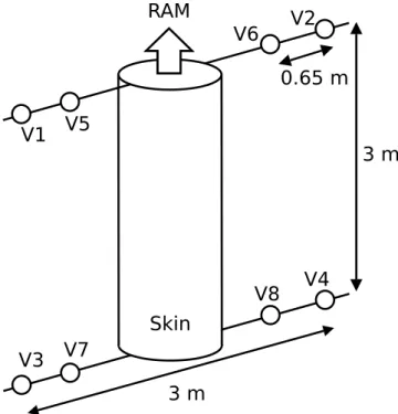
Fig. 1. MASS electric field probe arrangement. There were four booms with two probes each; two booms on the forward deck plate and two mounted on the aft deck plate. The 3′′ spherical probes
were coated with graphite paint. Voltage differences between pairs of probes, as well as the probe voltage relative to the rocket skin were telemetered.
Zahn et al., 2000), into NLC conditions to make a more comprehensive study of the phenomenon (Rapp et al., 2009; Robertson et al., 2009). In addition to allowing correlation studies between the ion densities and electric field within the cloud layer, the MASS and ECOMA rockets add to the vari-ety of conditions into which these instruments have flown. This diversity of environmental conditions is essential for testing theoretical models throughout the parameter space. The two MASS payloads carried identical hardware (Robert-son et al., 2009). The first flight went through moderate NLC and PMSE events, as observed by the ALOMAR lidar and ALWIN radar at Andøya rocket range, respectively; the sec-ond went through a somewhat weaker event. This paper will address the electric field fluctuations and conductivity mea-sured during the first MASS flight.
We show here that the probes measured the expectedv×B induced electric fields and spikes from shadowing of the probes by the rocket body. In addition, the probes moved about 1 V negative relative to the rocket body in the NLC re-gion, possibly due to impacts of negatively charged aerosols. The probes did not detect significant (>10 mV/m) DC fields and no wake effects were seen. We show that this small DC field perturbation is similar to that seen by the DROPPS 1 flight Holzworth et al. (2001). The electric field spectrum
was also found to be similar to the DROPPS 1 spectra from Pfaff et al. (2001), who suggested the turbulence was related to the strong PMSE radar reflections caused by structure at the Bragg scattering length. We also present a measure-ment of the upper bound of the conductivity of positive ions within the cloud layer. The measurement relies on the bot-tom boundary of the cloud layer being very sharp, and so the analysis cannot be extended to other datasets. However, the method works best within the cloud layer, which is a region that presents some difficulty for more conventional methods when large aerosols are present. We will report results on the order of 1×10⁻⁸S/m which are consistent with measure-ments made by Croskey et al. (2001) in similar conditions.
2 Instrumentation
Figure 1 shows the configuration of the electric field probes on both MASS payloads. The presence of two probes on each boom allows for several different probe separation pairs. The booms and probes were mechanically identical to those flown on the DROPPS flights (Holzworth et al., 2001). The electronics, though not identical to DROPPS, were similar. They consisted of a high-impedance preamp in each spheri-cal probe, followed by an amplifier module. Telemetry chan-nels included voltage differences between pairs of probes as well as between the probes and the rocket skin. All chan-nels were sampled with 12-bit accuracy, but sampling rates varied from 2 ksps to 33 ksps and gain varied from 0.25 to 10. Spatial resolution depends on the rocket velocity – about 1060 m/s – and was roughly 1 m–6 cm, depending on the sampling rate. Noise due to the electronics was only impor-tant in the least significant bit (0.6–23 mV, depending on the channel’s amplification). This technique has been used many times in ionospheric rocket measurements (Fahleson et al., 1970; Pfaff et al., 1984; Maynard, 1998; Holzworth et al., 2001).
3 Data 3.1 Overview
The MASS 1 flight (NASA designation 41.069) launched on 3 August 2007 at 22:51 UTC. The solar zenith angle was about 93◦, so the rocket was sunlit at the cloud altitude. Fig-ure 2 shows the PMSE observed by the ALWIN radar. There is a double-peak structure, with peaks at 83 km and 88 km. There were low-altitude clouds present at launch, and so we do not have lidar data of the launch conditions. However, NLC were detected by ALOMAR during breaks in the clouds before and after the launch (Baumgarten et al., 2009).
Fig. 2. ALWIN radar data for 3 August 2007 flight. T-0 was 22:51 UTC. Data and plot from Ralph Latteck at the Leibniz-Institut f¨ur Atmosph¨aren Physik.
– which points from V1 to V2 – is given by(V1−V2)/d12, whereV1is the voltage on probe V1, V2is the voltage on probe V2, andd12 is the distance between probes V1 and V2. Figure 3 shows thatE12,E15,E56, and E34 all mea-sure the same DC field – seen in the rotating rocket frame – despite having different probe separation distances. Spikes that are seen in all channels (for example, at 89.5 km, 90 km, 92.3 km, and 93.2 km) are caused by vibrations and/or gas re-leases from the attitude control system (ACS) valves. Small periodic deviations in theE15signal are possibly due to wake effects. Due to this rocket going slightly faster than expected, the booms were deployed closer to the bottom of the cloud than expected and vibrations in the booms did not dampen out quickly enough to observe the probes’ performance well below the NLC layer on the upleg portion. However, vi-brations are absent within the cloud layer, and the probes behaved similarly until increasing air resistance broke the booms off around 65 km on the downleg. Thus, the probes accurately measured DC electric fields both above the cloud, and – on the downleg – below the cloud as well.
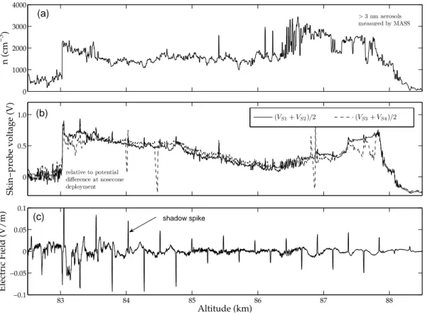
An overview of the aerosols and fields during the cloud passage is shown in Fig. 4. Figure 4a shows the charge density of the largest aerosols (>3 nm radii) measured by the MASS instrument, as a function of altitude (Robertson et al., 2009). Figure 4b shows the rocket skin voltage with respect to two sets of probes. The solid line is with respect to the average of the forward probes V1 and V2 – that is,
(VS1+VS2)/2 – and the dashed line is with respect to the average of the aft probes V3 and V4. Large spikes in the
VS3+VS4data at 84, 84.5, and 87 km seen in Fig. 4b are due to ACS valve firings. The onset of the cloud layer at 83 km
✂✁ ✂✄ ✄✆☎ ✝✆✞
Fig. 3. Electric fields measured by several pairs of probes over a 5 km region above the NLC layer. These are compared to the ex-pected inducedv×Belectric field, calculated using the measuredv
andB. The 2 Hz oscillation is due to rotation of the rocket. This
shows that different pairs of probes, with different probe separa-tions, in the front and aft of the rocket all measure the same expected DC electric field above the NLC event.
is very abrupt in the upper two panels, but the instruments resolve this rapid change with many data points during the transition. Notice that there are no large oscillations in the aft-probe data (VS3+VS4) as seen in DROPPS (Holzworth et al., 2001; Sternovsky et al., 2004). This may be due to the wake being smaller in this flight, or perhaps it was more symmetrically distributed about the rocket. Some differences between the forward and aft probes can be seen near 83 and 88 km, and are probably due to rocket wake effects. How-ever, these differences are significantly smaller than those modeled in Sternovsky et al. (2004).
Figure 4c showsE12, the forward electric field in the cloud layer. Thev×B electric field associated with the rocket ve-locity across the Earth’s magnetic field has been subtracted. The periodic sharp spikes are due to the probes rotating into the shadow of the rocket. The larger fluctuations at low al-titudes actually begin at lower alal-titudes than what is plot-ted, and include what looks like a smaller patch of particles below the main NLC event (Robertson et al., 2009). Data below 82 km is rather noisy, however – particularly in the forward channels – due to boom deployment being slightly higher in altitude than expected. Large fluctuations at the lower altitudes (83–85 km) of the cloud layer give way to smaller, higher frequency fluctuations in the middle altitudes (85–87 km). The top of the cloud layer shows weaker fluctu-ations.
✁✂✄✄ ☎✄✄✄ ✆✄✄ ✝✄✄✄
✞
✟
✡✠☞☛ ✁✄✠☞
✌✎✍✡✏✒✑✔✓✕✍✖✏✘✗✚✙✜✛✣✢ ✌✤✍✖✏✒✥✔✓✕✍✖✏✚✦✘✙✜✛✣✢
✧✆ ✧✄✝ ✧✄☛ ✧✄★ ✧✄✩ ✧✄✧
✪
✡✠✫✁
✪
✡✠☞✄☛ ✡✠☞✄☛ ✡✠✫✁
✬✮✭✰✯✲✱✴✳✶✵✸✷✺✹✲✻✺✹✲✼✽✻ ✱✰✵✸✳✶✻✺✾✲✷✺✵✸✿❁❀❃❂✰❄❆❅❈❇✶❇
(a)
(b)
(c) shadow spike
✷✺✵✸✼❉✳✲❊✺❋✽●❃✵❍❊✺✹❁■✚✹✲❊✺✵✸✯❃❊✺❋✽✳✲✼ ✿✶❋❉❏❑✵▲✷✺✵✸✯✲▼✸✵❍✳✶❊❈✯✲✹✶✻✺✵✸▼▲✹✶✯✲✵ ✿✶✵▲■✲✼❉✹❃❂✶✱❁✵▲✯❃❊
Fig. 4.An overview of the cloud layer. (a)Number densities of the heaviest aerosols measured by the MASS instrument, as a function of altitude (Robertson et al., 2009). (b)Change in the rocket-skin potential, with respect to the probe potential below the PMSE event, as a function of altitude. The solid line is with respect to the average of probes V1 and V2, and the dashed line is with respect to the average of probes V3 and V4. Notice how the profile follows the profile of the large negative aerosols. Large spikes in theVS3+VS4data at 84, 84.5, and 87 km are due to ACS valve firings. (c)TheE12 field, measured by probes V1 and V2 – that is, the field perpendicular to the rocket
velocity. Thev×Belectric field associated with the rocket velocity across the Earth’s magnetic field has been subtracted. The sharp, periodic
spikes are shadowing spikes, caused by the probe moving into the shadow of the rocket.
✂✁ ☎✄ ✝✆ ☎✞
Fig. 5.A high time-resolution view of the onset of the NLC layer in Fig. 4b. The transition takes less than 10 ms, over much of which the potential varies linearly with time/altitude. There is a delay between the forward and aft channels of about 2.5 ms, which is roughly the time it takes for the aft probes to “catch up” to where the forward probes were (at the rocket velocity of about 1 km/s).
Comparing 4a and 4b, one can see that the shapes of the two curves are similar. There is a sharp ledge at 83 km, fol-lowed by a slow decrease, though it remains elevated relative to the value below the cloud. It starts increasing again above 86 km, and then drops back down by 88 km. The ampli-tude of the shadowing spikes also follows this general profile. This suggests that the skin-to-probe voltage and shadowing spike amplitudes are driven by the density of large charged aerosols.
3.2 Rapid potential changes
forward probes were (at the rocket velocity of about 1 km/s). These two observations suggest that the onset of the NLC layer is very sharp: less than the 3 m vertical probe separa-tion. If it were not sharp, or if the feature was due to a shift in the rocket-skin potential, there would not be a delay in the two signals. If the change in the skin-to-probe voltage is due primarily to changes in the probes, then it means the probes are becoming charged negative within the NLC layer. The similarity between the shape of the plot showing the probe voltage versus altitude and the density of large negatively charged aerosols (Figs. 4a and 4b) supports this interpreta-tion. This is not unexpected, since a much greater fraction of the probes’ surface area was exposed to the aerosols, as compared to the rocket body, which was aligned along the ram direction.
3.3 Probe shadowing
Figure 4c showsE12 versus altitude, with thev×Belectric field subtracted, as discussed above. The shadowing spikes occur when the probes enter the rocket’s shadow. Within the rocket’s shadow the photocurrent stops, which causes the shadowed probe to become more negative. The profile of the spike amplitudes has a similar shape to both the heavy charged aerosol densities (Fig. 4a) and the skin-to-probe volt-age (Fig. 4b). That is, the spikes suddenly increase in am-plitude around 83 km, then reduce significantly in amam-plitude near 86 km, grow again above 86 km, and are dramatically reduced above 88 km.
Probe voltages are determined by current balance. Over periods longer than the local relaxation time, the probes should be in current balance. The net current to the probes is zero, so that
X
I =Iγ+Ia+Ie+Ii =0, (1)
whereIγis the photocurrent,Iais the current due to incident aerosols,Ie is the electron thermal current, andIi is the ion current (Maynard, 1998). The current drawn by the electron-ics is negligible.
The electron current is non-linear with voltage, but through much of the cloud layer, the ion current can be ap-proximated as linear as in the IV curve seen by a low voltage Gerdien condenser in an NLC (Croskey et al., 2001). This is especially true if we consider only the differential con-ductivity,σ=1I /1V, as a perturbation of the sunlit state. In the following, we will assume Ii is approximately lin-ear with probe voltage. Thus, 1Ii is approximately de-scribed by Ohm’s law: J=σ E. SubstitutingJ=I /(4π r2)
andE=−V /rfor conducting spheres – whereris radius of the spheres – we have
1Ii = −4π rσ Vprobe= −1(Iγ +Ia+Ie). (2) Below the NLC layer, the photocurrent is dominant, and we expect the probe voltage to be positive with respect to the
lo-cal space potential. Above the NLC layer, the electron ther-mal current is dominant. In both cases, the dominant voltage-dependent current to the probes is carried by electrons. As such, the probe potential should be close to the local space potential, since the electrons have a high conductivity. This is consistent with data above the cloud layer (Fig. 4c, above 88 km).
Outside of the cloud, Ia is negligible. Within the cloud layer, however, the charged aerosol density – and Ia – is large enough that it cannot be ignored. When the probe is in the rocket shadow, the photocurrent vanishes and the net voltage-independent current is negative. The ambient elec-trons are cold –kT /qeis about 12 mV – so the electron ther-mal current is negligible when the probe potential is less than the local space potential. Thus, during the shadowing spikes the return current is carried primarily by positive ions. Since the conductivity of ions is so much lower than for electrons, the shadowing spike amplitudes are much larger within the cloud. This also allows us to use the shadowing spike ampli-tude to approximate the potential difference due to the nega-tive aerosol current.
An alternative analysis is to treat Ii, Ie, Ia, and Iγ as known (or calculable via a model), and to solve for the elec-tron density that yields the correct shadowing spike ampli-tudes. In such a model, however, small electron densities are required for large shadowing spike amplitudes (and vice versa). PMSE peaks were measured at 83 km and 88 km, where the shadowing spikes were largest. In a double-layer PMSE event, one expects an electron density profile which has a minimum between the two peaks, where the radar re-flection is weaker, instead of 2 minima co-located with the peaks. We nonetheless applied such a model, which calcu-lated an electron density of 12 cm−3at 83 km. It is unlikely that such a low electron density could support the PMSE measured there.
With that in mind, we continue trying to estimate the posi-tive ion conductivity. It is important to know when the probes are in current balance. Figure 6 is a high resolution compari-son of a tip-to-tip probe pair,V12, and a same-boom probe pair, V15, which shows that the probes reach current bal-ance. First, probe V5 enters the shadow, which lowers its potential and increases the V15 potential difference. Then, probe V1 enters the shadow, which lowers its potential and decreases bothV15 andV12. Notice thatV15 nearly returns to the same value it had before V5 entered the shadow. Af-terwards, probes V1 and then V5 leave the shadow, reversing the voltage shifts.
✂✁ ✂✄
Fig. 6.High time resolution comparison ofV12andV15at a
shad-owing spike around 87 km. Probe V2 is in sunlight the entire time. V5 goes into the rocket shadow first – raising theV15potential
dif-ference – followed by V1. The probes are nearly settled in voltage, which shows that the current balance is attained within the rocket shadow. Below about 84.5 km, the conductivity is too low and the probes do not reach equilibrium, although the shadowing spike am-plitudes are larger.
✁
Fig. 7. Positive ion conductivity calculated from the shadowing spike amplitudes and aerosol densities. Points below about 84.5 km over-estimate the conductivity, since the shadowing spikes do not quite reach equilibrium within the rocket shadow. If there were other significant return currents present, they would inflate the cal-culated conductivity values. As such, this reflects the maximum value one could expect the ion conductivity to have.
to the probe via
I =C 1V /1t, (3)
and compare that to the number of particles measured by MASS at that altitude (Fig. 4a) to get an effective “effi-ciency” of charge collection,
ε=Ia/na(83 km). (4)
We then extrapolate to estimate Ia at other altitudes using Fig. 4a:Ia≈ε na. This estimation, with shadowing spike am-plitudes from Fig. 4c, yields an estimated positive ion con-ductivity,
σ =ε na/4π r Vprobe, (5)
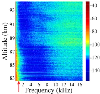
Fig. 8. Spectrogram ofE12 around the PMSE layer. The layer
can be seen around 83–88 km. The high-frequency fuzz is probably auroral hiss, which shows that the instrument accurately measured high frequency signals.
where the shadowing spike amplitudes are used forVprobe. SubstitutingC=4π ǫ0
1
r−
1
r+λD
−1
and Eq. (4) into Eq. (3) (whereλDis the Debye length), this becomes
σ = 1V 1t
na
na(83 km)
ǫ0
Vprobe
1− r
r+λD
−1
. (6)
Figure 7 shows the results of this calculation. The overall values are within a factor of 2 of those measured by Croskey et al. (2001) on DROPPS 1. Note that below about 84 km, the values level off, as is expected, given that the probes did not reach equilibrium there. Also, if there were other signifi-cant return currents present, they would inflate the calculated conductivity values. As such, Fig. 7 reflects the maximum value one could expect the ion conductivity to have.
3.4 AC fluctuations
Other channels look very similar. One might expect to see a difference in spectra between spin-plane channels and rocket-axis channels, since PMSE exhibit strong aspect sen-sitivity (Czechowsky et al., 1988). However, no easily identi-fiable differences were seen. This is not entirely unexpected, since the rocket was angled approximately 30◦off of the ver-tical. Thus, both spin-plane and rocket-axis channels con-tained significant vertical and horizontal components.
There are also broad bands of VLF hiss, which could be auroral hiss. Banding in time/altitude is due to the rocket rotation. Within the cloud layer the hiss appears to have a lower frequency cutoff of about 8 kHz. The cloud layer ap-pears to attenuate the hiss, since above it the signal is some-what stronger overall, and the lower cutoff is around 4 kHz. Though this hiss is unrelated to the NLC layer, it supports the conclusion that the probes measured geophysical VLF signals. Pfaff et al. (2001) observed similar signals in the DROPPS campaign.
Figure 9 shows a power spectral density of theE15electric field measured within the electron “bite-out” region from 85– 87 km. There is a “knee” in the spectrum around 250 Hz, which corresponds to a spatial scale of about 4 m. The probe separation is about 0.65 m, so boom length effects should be marginal at those spatial scales. The spectrum ofE24 has similar features. We expect structures to extend to these short scales, since radar reflects most strongly off features at the Bragg scale. Our spectrum is similar to spectra measured by Pfaff et al. (2001) on DROPPS.
4 Conclusions
We have presented high time-resolution E-field data in a NLC event. Similar to the DROPPS 1 rocket flight into a weak NLC, the MASS rocket flights found only weak DC electric field perturbations in the cloud. This finding contra-dicts theories which require large electric fields for the for-mation or maintenance of NLC conditions. The density pro-file of the heaviest aerosols measured by the MASS instru-ment had a similar shape to the skin-to-probe voltage. Such a strong similarity suggests that the skin-to-probe voltage was, at least within the cloud layer, perturbed by incident heavy charged aerosols. The probes measured a very sharp bound-ary at the lower edge of the NLC layer, in which the signal from the aft probes was delayed with respect to the forward probes caused by their 3 m separation. Thus, the structures seen in the skin-to-probe voltage are due to changes in the probe potential rather than the rocket skin potential. Similar potential shifts, in which the skin-to-probe voltage increased within the NLC event, were also seen in the DROPPS E-field data, and it is likely that those were likewise due to changes in the probe potential.
Spikes in the probe potential due to probe shadowing were observed in both MASS flights as well as both DROPPS flights. In DROPPS, the mechanisms controlling the
am-10 100 1,000 4,000
−130 −120 −110 −100 −90 −80 −70
Frequency (Hz)
10
lo
g1
0
(P
S
D
),
(V
/m
)
2 /H
z
1 10
100
Scale along rocket trajectory (m)
Fig. 9. Power spectral density (PSD) ofE15 within the electron bite-out region. To remove probe shadowing artifacts from the data, spectra were calculated for the regions between the shadowing spikes. TheE15channel was used because the shadowing spikes
occur half as often as in theE12data. There is a “knee” in the spec-trum around 250 kHz, which corresponds to a spatial scale of 4 m.
plitude of the spikes were unknown. With the first MASS flight, however, the sharpness of the NLC layer’s onset and the presence of the MASS instrument provided us with some unique calibration opportunities. Our calibration yielded re-sults in rough agreement with those found in Croskey et al. (2001), despite using a completely different method. This was a non-trivial task, since the probes are designed to be used for difference measurements, whereas the calculation of conductivity largely relied on single-ended data.
Acknowledgement. This research was supported by NASA grant NNG05WC55G at the University of Washington, the Wallops Flight Facility of NASA, and the Andøya Rocket Range. We would also like to thank Ralph Latteck for Fig. 2.
Topical Editor C. Jacobi thanks M. Friedrich and M. Rapp for their help in evaluating this paper.
References
Ann. Geophys., 27, 953–965, 2009, http://www.ann-geophys.net/27/953/2009/.
Blix, T. A., Bekkeng, J. K., Latteck, R., L¨ubken, F.-J., Rapp, M., Sch¨och, A., Singer, W., Smiley, B., and Strelnikov, B.: Rocket probing of PMSE and NLC – results from the recent MI-DAS/MaCWAVE campaign, Adv. Space Res., 31, 2061–2067, doi:10.1016/S0273-1177(03)00229-1, 2003.
Cho, J. Y. N. and Kelley, M. C.: Polar mesosphere summer radar echoes: observations and current theories, Rev. Geophys., 31, 243–265, 1993.
Cho, J. Y. N. and R¨ottger, J.: An updated review of polar meso-sphere summer echoes: Observation, theory and their relation-ship to noctilucent clouds and subvisible aerosols, J. Geophys. Res., 102, 2001–2020, 1997.
Croskey, C. L., Mitchell, J. D., Friedrich, M., Torkar, K. M., and Goldberg, R. A.: Charged particle measurements in the polar summer mesosphere obtained by the DROPPS sounding rockets, Adv. Space Res., 28, 1047–1052, 2001.
Czechowsky, P., Reid, I. M., and R¨uster, R.: VHF radar measure-ments of the aspect sensitivity of the summer polar mesopause echoes over Andenes (69◦N, 16◦E), Norway, Geophys. Res.
Lett., 15, 1259–1262, 1988.
D’Angelo, N.: IA/DA waves and polar mesospheric summer echoes, Phys. Lett. A, 336, 204–209, doi:10.1016/j.physleta. 2005.01.037, 2005.
Ecklund, W. L. and Balsley, B. B.: Long-Term Observations of the Arctic Mesosphere With the MST Radar at Poker Flat, Alaska, J. Geophys. Res., 86, 7775–7780, 1981.
Fahleson, U. V., Kelley, M. C., and Mozer, F. S.: Investigation of the operation of a d.c. electric field detector, Planet. Space Sci., 18, 1551–1561, 1970.
Goldberg, R. A., Kopp, E., Witt, G., and Swartz, W. E.: An overview of NLC-91: a rocket/radar study of the polar summer mesosphere, Geophys. Res. Lett., 20, 2283–2286, 1993. Holzworth, R. H. and Goldberg, R. A.: Electric field measurements
in noctilucent clouds, J. Geophys. Res., 109, D16203, doi:10. 1029/2003JD004468, 2004.
Holzworth, R. H., Pfaff, R. F., Goldberg, R. A., Bounds, S. R., Schmidlin, F. J., Voss, H. D., Tuzzolino, A. J., Croskey, C. L., Mitchell, J. D., von Cossart, G., Singer, W., Hoppe, U.-P., Murtagh, D., Witt, G., Gumbel, J., and Friedrich, M.: Large Electric Potential Perturbations in PMSE During DROPPS, Geo-phys. Res. Lett., 28, 1435–1438, 2001.
Latteck, R., Singer, W., and Bardey, H.: The ALWIN MST radar: technical design and performance, in: Proceedings of the 14th ESA Symposium on European Rocket and Balloon Programmes and Related Research, pp. 179–184 (ESA SP–437), Potsdam, Germany, 1999.
Lie-Svendsen, Ø., Blix, T. A., Hoppe, U.-P., and Thrane, E. V.: Modeling the plasma response to small-scale aerosol particle per-turbations in the mesopause region, J. Geophys. Res., 108, 8442, doi:10.1029/2002JD002753, 2003a.
Lie-Svendsen, Ø., Blix, T. A., Hoppe, U.-P., and Thrane, E. V.: Modeling the small-scale plasma response to the presence of heavy aerosol particles, Adv. Space Res., 31, 2045–2054, 2003b. L¨ubken, F.-J., Rapp, M., and Hoffmann, P.: Neutral air tur-bulence and temperatures in the vicinity of polar mesosphere summer echoes, J. Geophys. Res., 107, 4273, doi:10.1029/ 2001JD000915, 2002.
L¨ubken, F.-J., Baumgarten, G., Fiedler, J., Gerding, M., H¨offner, J., and Berger, U.: Seasonal and latitudinal variation of noctilucent cloud altitudes, Geophys. Res. Lett., 35, L06801, doi:10.1029/ 2007GL032281, 2008.
Maynard, N. C.: Electric field measurements in moderate to high density space plasmas with passive double probes, in: Measure-ment Techniques in Space Plasmas: Fields, edited by: Pfaff, R. F., Borovsky, J. E., and Young, D. T., pp. 13–27, American Geophysical Union, Washington DC, 1998.
Pfaff, R., Holzworth, R., Goldberg, R., Freudenreich, H., Voss, H., Croskey, C., Mitchell, J., Gumbel, J., Bounds, S., Singer, W., and Latteck, R.: Rocket probe observations of electric field irregular-ities in the polar summer mesosphere, Geophys. Res. Lett., 28, 1431–1434, 2001.
Pfaff, R. F., Kelley, M. C., Fejer, B. G., Kudeki, E., Carlson, C. W., Pedersen, A., and Hausler, B.: Electric field and plasma den-sity measurements in the auroral electrojet, J. Geophys. Res., 89, 236–244, 1984.
Rapp, M. and L¨ubken, F.-J.: Polar mesosphere summer echoes (PMSE): Review of observations and current understanding, At-mos. Chem. Phys., 4, 2601–2633, 2004,
http://www.atmos-chem-phys.net/4/2601/2004/.
Rapp, M. and Thomas, G. E.: Modeling the microphysics of meso-spheric ice particles: Assessment of current capabilities and ba-sic sensitivities, J. Atmos. Sol.-Terr. Phys., 68, 715–744, doi: 10.1016/j.jastp.2005.10.015, 2006.
Rapp, M., Strelnikova, I., Strelnikov, B., Latteck, R., Baumgarten, G., Li, Q., Megner, L., Gumbel, J., Friedrich, M., Hoppe, U.-P., and Robertson, S.: First in situ measurement of the vertical distribution of ice volume in a mesospheric ice cloud during the ECOMA/MASS rocket-campaign, Ann. Geophys., 27, 755–766, 2009, http://www.ann-geophys.net/27/755/2009/.
Robertson, S.: Relationship of electric field and charged particle density fluctuations to air turbulence in the mesosphere, J. Geo-phys. Res., 112, D20203, doi:10.1029/2007JD008412, 2007. Robertson, S., Hor´anyi, M., Knappmiller, S., Sternovsky, Z.,
Holz-worth, R., Shimogawa, M., Friedrich, M., Torkar, K., Gumbel, J., Megner, L., Baumgarten, G., Latteck, R., Rapp, M., and Hoppe, U.-P.: Mass analysis of charged aerosol particles in NLC and PMSE during the ECOMA/MASS campaign, Ann. Geophys., in press, 2009.
Sternovsky, Z., Holzworth, R. H., Hor´anyi, M., and Robertson, S.: Potential distribution around sounding rockets in mesospheric layers with charged aerosol particles, Geophys. Res. Lett., 31, L22101, doi:10.1029/2004GL020949, 2004.
Strelnikov, B., Rapp, M., Blix, T. A., Engler, N., H¨offner, J., Laut-enbach, J., L¨ubken, F.-J., Smiley, B., and Friedrich, M.: In situ observations of small scale neutral and plasma dynamics in the mesosphere/lower thermosphere at 79◦N, Adv. Space Res., 38,
2388–2393, doi:10.1016/j.asr.2005.03.097, 2006.
von Zahn, U., von Cossart, G., Fiedler, J., Fricke, K. H., Nelke, G., Baumgarten, G., Rees, D., Hauchecorne, A., and Adolfsen, K.: The ALOMAR Rayleigh/Mie/Raman lidar: objectives, configu-ration, and performance, Ann. Geophys., 18, 815–833, 2000, http://www.ann-geophys.net/18/815/2000/.