Tube Model Predictive Control with an Auxiliary Sliding Mode Controller

Tube Model Predictive Control with an Auxiliary

Sliding Mode Controller

Miodrag Spasi´

c

Morten Hovd

Darko Miti´

c

Dragan Anti´

c

1_{Department of Control Systems, Faculty of Electronic Engineering, University of Niˇs, Serbia.}

E-mail: {Miodrag.Spasic, Darko.Mitic, Dragan.Antic}@elfak.ni.ac.rs

2_{Department of Engineering Cybernetics, Norwegian University of Science and Technology, Trondheim, Norway.}

E-mail: {Morten.Hovd, Miodrag.Spasic}@itk.ntnu.no

Abstract

This paper studies Tube Model Predictive Control (MPC) with a Sliding Mode Controller (SMC) as an auxiliary controller. It is shown how to calculate the tube widths under SMC control, and thus how much the constraints of the nominal MPC have to be tightened in order to achieve robust stability and constraint fulfillment. The analysis avoids the assumption of infinitely fast switching in the SMC controller.

Keywords: Model Predictive Control, robustness, Sliding Mode Control, Mixed Integer Linear Program

1. Introduction

Model Predictive Control (MPC) has been a great in-dustrial success, particularly in the process industries (Qin and Badgwell, 2003). Still, robustness of MPC controllers continues to be an active research issue. There are many approaches to robust MPC, includ-ing dynamic programminclud-ing, optimization over feedback policies, min-max MPC, etc. Providing an overview over these various approaches to robust MPC is be-yond the scope of this paper, the interested reader is instead referred to the bibliographic notes in Chap-ter 3 of Rawlings and Mayne (2009). As is noted in (Rawlings and Mayne, 2009), optimal or close-to-optimal approaches to robust MPC generally have pro-hibitive online calculation requirements. More prac-tical approaches are therefore a compromise between performance and online calculation requirements.

A popular approach among such MPC formulations that trade off performance against online calculation requirements is the so-called Tube MPC (Rawlings and Mayne, 2009). In the ’basic’ Tube MPC, the MPC controller essentially controls the nominal plant, while there is an auxiliary controller that keeps ’all possible’

computational requirements of the Sliding Mode Con-trol (SMC) are trivial, and combined with the good robustness properties of SMC this should make SMC an attractive candidate for the auxiliary controller in Tube MPC.

SMC is known for its robustness to parameter vari-ations and external disturbances. It belongs to a special class of nonlinear discontinuous control algo-rithms, known as variable structure control (Utkin, 1978; Young et al., 1999; Yu and Kaynak, 2009). In its basic form, the SMC input is simply a relay out-put, depending on the location of the present state relative to a switching surface, which forces a system state to move along this surface, known also as a slid-ing surface. The modern realization of SMC, by usslid-ing microcontrollers or digital signal processors, causes a quasi-sliding motion (Milosavljevi´c, 1985) usually in O(T) vicinity of sliding surface, with T denoting a sampling time, which could induce a chattering, mani-fested by high-frequency control signal exciting unmod-elled system dynamics and reducing plant lifecycle. An overview of existing digital SMC algorithms is given in (Milosavljevi´c,2004).

In recent years, researchers have developed several control methodologies based on the combination of SMC and MPC. The combination of SMC and general-ized predictive control (GPC), as a subclass of MPC, is discussed in (Corradini and Orlando,1997;Miti´c et al., 2013) for systems with discrete-time transfer function models. In (Garcia-Gabin et al., 2009) the cost func-tion is partially optimized with respect to only the pre-dictive part of controller, while sliding mode control is not involved in the optimization problem. More-over, the reaching and existence conditions of sliding mode are not derived and the stability issues are not discussed. Unfortunately, all these approaches cannot deal with MIMO systems.

In digital SMC based on state-space models, and hence applicable to MIMO systems, one approach to control law design is to force the system to reach the sliding surface at the very next sampling instant (Su et al., 2000). This digital SMC method provides a

O(T2_{) sliding mode accuracy when the system} distur-bances are known at each time instant or a unit-step delayed disturbance estimate is used in the presence of unmodeled disturbances. However, when the dis-turbance depends on the control input, the system be-comes unstable or causes chattering. That is why two different approaches in integrating digital SMC and MPC are proposed in (Neelakantan, 2005). The first one applies direct optimization of a cost function crite-rion with respect to the equivalent control. The second control method splits the controller into the equivalent control part, ensuring the system to stay on sliding

sur-face once reached, and the reaching control part that guides the system towards the sliding surface. The cost function is optimized with respect to the latter control term.

In (Incremona et al.,2015;Benattia et al.,2015) hi-erarchical control schemes, consisting of a high level MPC and a low level SMC (Rubagotti et al., 2011), are considered. The role of the SMC component is to reject the matched disturbances acting the plant, and to reduce uncertainty for the MPC design in that way. The accurate calculation of the tube widths is com-plicated even when using linear state feedback. A set of states needs to be calculated, inside which the auxil-iary controller is able to keep the states of the real sys-tem. Once this set is calculated, the corresponding set inside which the input from the auxiliary control will remain has to be calculated. To avoid restricting the nominal MPC unnecessarily, the calculated set should be as small as possible,i.e, we wish to calculate the so-called minimal robustly positive invariant set (mRPI) for the system under the auxiliary control. Unfortu-nately, the mRPI will typically be excessively complex and demanding to calculate, but good outer approxi-mations can usually be found when linear state feed-back is used as an auxiliary controller (Rakovi´c et al., 2005).

To the authors’ knowledge, there is no previous work on calculating robustly positively invariant sets for sys-tems under SMC control with a finite sampling fre-quency for the SMC. However, we will also take an al-ternative approach: following an idea inRawlings and Mayne(2009), the robustly positively invariant set will not be calculated directly. Instead, we will show how to calculate, for each constraint, how far in the direc-tion of the constraint the true system can be driven by the model uncertainty. This will give a direct measure of how much each constraint will need to be tightened. Tube MPC was originally proposed with the MPC handling the nominal system only, and the auxiliary controller handling the deviations from nominal behav-ior. Alternative formulations have been proposed later, where feedback is introduced also into the MPC part of Tube MPC. In this paper, including the example, we have chosen to use a nominal Tube MPC as in the orig-inal Tube MPC formulation, in order to highlight the robustness improvement from the auxiliary controller. However, the SMC-based auxiliary controller proposed in the paper would be equally applicable to a Tube MPC formulation where feedback is used also in the MPC part of the Tube MPC.

con-straints tightening is presented in Section 4. The pro-posed Tube MPC with an auxiliary SMC has been applied to the real DC servo system (Inteco, 2011), and the digital simulation and experimental results are given in Section5. Section6contains some concluding remarks.

2. Problem description

Consider the discrete time system described by the model

xk+1=Axk+Buk+Ewk, (1)

with the system statex∈Rnx_{, the inputu∈R}nu_{, and}

the disturbance w ∈ Rnw_{. There are also constraints}

on the allowable state

x∈X_{={x|F x≤f}, (2)}

constraints on the allowable input

u∈U_{={u|Γu≤γ}, (3)}

and constraints on the possible range of disturbances

w∈W_{={w|Hw≤h}. (4)}

It follows from the description above that the setsX_,U_, and W _{are polyhedral; we will also assume that they} are bounded (and thus that the sets are polytopic), of full dimension, and contain the origin in their interior. In the following, the system state is split into two components, a nominal component z and a deviation from nominalǫ

x=z+ǫ. (5)

Similarly, the input is split into the input from the nominal MPC v, and the input ν from the auxiliary controller

u=v+ν. (6)

The dynamics, described by eq. (1), may therefore be split into the nominal dynamics and the deviation from nominal

zk+1= Azk+Bvk (7)

ǫk+1= Aǫk+Bνk+Ewk (8)

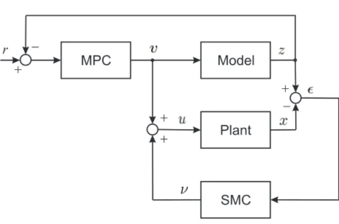
Clearly, eqs. (7) and (8) add to eq. (1). The control scheme is illustrated in Figure 1.

At each timestep, the nominal MPC solves the prob-lem

min

z,v

J(z_,v_{) (9)}

subject to

zk+i ∈ {zk+i|F zk+i ≤f −δiz} i∈ {0,1, . . . , N},

vk+i∈ {vk+i|Γvk+i≤γ−δvi} i∈ {0,1, . . . , N}.

Model

Plant

SMC MPC

+

+

+

-+

r

Figure 1: Control scheme

Here, J(z_,v_{) is the MPC cost function}1_{, N is the}

length of the prediction horizon for the MPC, z _is

the vector of present and future nominal states in the prediction horizon, zT ₌

zT

k zTk+1 . . . zkT+N

, and

v _{is the vector of present and future inputs from}

the nominal MPC in the prediction horizon, vT ₌

vT

k vTk+1 . . . vkT+N

. The vector δz

i quantifies how

much the nominal state constraints have to be re-stricted at time k+iin order to ensure that the true state adheres to the original constraints, while the vec-torδv

i quantifies how much the constraints on the

nom-inal MPC input have to be restricted at timek+iin order to ensure that the total input adheres to the orig-inal constraints. The simplest Tube MPC formulations treatδz

i and δiv as constants over the prediction

hori-zon, whereas other formulations allow these to vary to account for the fact that the disturbance will typ-ically be able to drive the true state further from the nominal state (also under the action of the auxiliary control) over a time period of several timesteps than over a single timestep.

Remark_{. A special terminal set for the state is a}

common ingredient in MPC formulations guaranteeing closed loop stability. Such a terminal set is ignored in eq. (9) for reasons of notational simplicity, but it adding such a terminal set would be straight forward.

From eq. (9), it is clear that δz

i and δiv have to be

found in order to be able to formulate the nominal MPC. This will be addressed in Section4.

3. Digital Sliding Mode Control

To design the auxiliary digital SMC, we consider the deviated system dynamics described by eq. (8). Two

1_{The cost function will not be specified at present, but we do}

control algorithms are implemented herein. The first one is a traditional relay based sliding mode control defined by

νk=−(KB)−1(KAǫk−gk+ ∆usign(gk)) (10)

where

gk =Kǫk (11)

denotes switching function and

gk = 0 (12)

is the equation for the sliding surface or the intersection of sliding surfaces ifnu>1 . Notice thatKǫkis usually

selected as an auxiliary control in Tube MPC and a matrix K has dimension nu ×nx. Here sign(gk) is

understood to be a vector with elements ±1, and ∆u

is a diagonal matrix with constants representing the relay outputs. The sliding surface, i.e. K, should be selected so that the system (Furuta,1990)

ǫk+1 = (A−B(KB)−1K(A−I))ǫk (13)

Kǫk = 0 (14)

is stable. Eqs. (13) and (14), describing system dy-namics in sliding mode, are obtained by implementing the well-known equivalent control

νeqc_k =−(KB)−1_(KAǫ

k−gk) (15)

in eq. (8). Substituting eq. (10) in eqs. (8) and (11) yields

gk+1=gk−∆usign(gk) +KEwk (16)

defining the switching function dynamics at time in-stant k, whereas in the prediction horizon it is deter-mined by

gk+i+1 = gk+i−∆usign(gk+i) +KEwk+i,(17)

i ∈ {0,1, . . . , N}

In order to provide stable switching function dynam-ics, ∆ushould be calculated according to the following

theorem.

Theorem 3.1. _{If∆uis chosen to satisfy the following} inequality

∆u1>Ω>max|KEwk|, (18)

whereΩis a positive real vector and1is a vector of 1’s, then, for every initial state gk, there exists a positive

integer number k0 = k0(gk) < N, such that the

sys-tem phase trajectory, described by eqs. (17) and (18), enters the domain defined by

G={gk+i:|gk+i|<∆u1 + Ω}, (19)

after k0 time steps and remains in this domain for all

i > k0.

Proof. See AppendixA.

The second auxiliary digital SMC, used in this paper, is so-called robust discrete-time chattering free sliding mode control (Golo and Milosavljevi´c, 2000)

νk= − (KB)−1 KAǫk−gk (20)

+ min(I|gk|,∆u)sign(gk)

Implementing eq. (20) in eq. (8), the switching func-tion dynamics becomes

gk+1=gk−min(I|gk|,∆u)sign(gk) +KEwk (21)

and, inside the prediction horizon, we have

gk+i+1 = gk+i−min(I|gk+i|,∆u)sign(gk+i)

+ KEwk+i, i∈ {0,1, . . . , N} (22)

The next theorem gives sufficient conditions for stable sliding motion in prediction horizon.

Theorem 3.2. _{The system phase trajectory, described} by eqs. (22) and (18), reaches the domain G defined by eq. (19) in k0 =k0(gk) < N time steps for every

initialgk, and remains in it for alli > k0.

Proof. See AppendixB.

4. Calculating the required

constraint tightening with

SMC-based auxiliary controllers

We will first describe how to calculate the required con-straint tightening with control defined by eq. (10). However, relay feedback is known to often result in very fast switching, which for some applications will not be desirable. A common remedy is then to replace the ’infinite gain’ at the switching surface with a steep linear function, leading to a chattering free SMC de-scribed by eq. (20). The second subsection will address the constraint tightening for this type of auxiliary con-troller.

It is noted above that an auxiliary controller with low calculation requirements may operate at a higher sampling rate (shorter timestep) than the MPC. How-ever, we will use the same sampling frequency both for MPC and SMC.

With the simple SMC-inspired auxiliary controllers considered here, the determination of δv

i is trivial,

which will become apparent below. However, the cal-culation ofδz

4.1. Constraint tightening for traditional

SMC

Denote the relay term in eq. (10) as

ϑk = ∆usign(Kǫk), (23)

To proceed, we define for each element ϑj of ϑ a

binary variable sj, such that ϑj > 0 ⇒ sj = 1, and

sj = 0 otherwise. Also needed are upper and lower

bounds on each component of the vectorKǫ. From eqs. (2) and (5), it is clearly safe to assume F ǫ ≤f, and the lower boundsmj and upper boundsµj on element

j ofKǫcan be found from the LPs

mj = min

F ǫ≤fKjǫ (24)

and

µj = max

F ǫ≤fKjǫ (25)

where Kj is row j ofK. Let 1 denote a vector of 1’s.

Equation (23) is then implied byMignone(2001)

ϑk = ∆uS−∆u(1−s) = ∆u(2s−1), (26)

where the value of the binary variables s follow from the constraints

mj(1−sj)< Kjǫ (27)

−µjsj< −Kjǫ (28)

Note that numerical optimization solvers cannot dis-tinguish between strict and non-strict inequalities. The formulation above will leave the value ofsj undecided

if Kjǫ = 0. It will then be left for the optimization

routine to choose the optimal value.

The furthest from the origin the disturbance se-quence {wk} may drive the deviation state ǫk in the

direction of the state constraintFlxk≤fl over a

hori-zon ofN timesteps can then be found by solving

δfj,N = maxwk,sk,ǫkFlǫN (29)

subject to

ǫ0= 0

Hwk≤h; k= 0, . . . , N−1

ǫk+1=Aǫk+B∆u(2sk−1) +Ewk;

k= 0, . . . , N−1

A=A−B(KB)−1_K(A−I)

B =−B(KB)−1

diag{mj}(1−sk)< Kǫk; k= 0, . . . , N −1

−diag{µj}sk<−Kǫk; k= 0, . . . , N−1

sk∈ {0,1}nu

For each state constraint j, this optimization should be solved for a number of horizon lengthsN. For each timestepi, the elements ofδz

i are given byδfj,i. If the

system under the relay feedback is stable, δfj,N will

approach an upper bound asN grows large.

4.2. Constraint tightening for chattering

free SMC

Instead of eq. (23) we now use

ϑj=min(|Kjǫ|,∆uj)sign(Kjǫ) (30)

where ∆ujdenotes thej’th element on the main

diago-nal of the diagodiago-nal matrix ∆u, andKj as before refers

to rowj ofK. We rewrite eq. (30) as

ϑj = sat(Kjx) =







∆uj ifKjǫ≥∆uj

Kjǫ if −∆uj≤Kjǫ≤∆uj

−∆uj ifKjǫ≤ −∆uj

(31) To capture this behavior, we need two binary variables,

sj andtj for each auxiliary inputϑj, such that

Kjǫ <−∆uj →sj = 0 (32)

Kjǫ >−∆uj →sj = 1 (33)

Kjǫ <∆uj →tj= 0 (34)

Kjǫ >∆uj →tj= 1 (35)

Define

qj=Kjǫ−mj (36)

where mj is calculated as in eq. (24). We note that

qj is non-negative in the domain of interest. The

ac-tual input from the auxiliary controller may then be calculated from the expression

ϑj =−(1−sj)∆uj+ (sj−tj)(qj+mj) +tj∆uj (37)

where we note that sj ≥ tj. The difficulty in the

above equation lies in the bilinear termssjqj andtjqj,

both being the product of a binary variable and a non-negative real. To proceed, we introduce the auxiliary variables σj = sjqj and τj = tjqj. From (Bemporad

and Morari, 1999), we have that the set

R={(qj, sj, σj) :σj=sjqj,0≤qj≤aj, sj∈ {0,1}}

(38) can equivalently be expressed as

M= {(qj, sj, σj) : 0≤σj ≤ajsj, (39)

qj+ajsj−aj≤σj≤qj, sj∈ {0,1}}

and similarly for (qj, tj, τj). Recognizing that in this

caseaj =µj−mj, and introducing

m1j =mj+ ∆uj (40)

µ1j =µj+ ∆uj (41)

m2j =mj−∆uj (42)

Defining the diagonal matrices Λ = diag(aj), M1 = diag(m1j), ¯M1 = diag(µ1j), M2 = diag(m2j), and

¯

M2= diag(µ2j), and forming the column vectorsm=

vec(mj), sk = vec(skj), tk = vec(tkj), σk = vec(σkj),

and τk = vec(τkj), we obtain the optimization

formu-lation

δfl,N =maxwk,ϑk,σk,τk,sk,tk,ǫkFlǫN (44)

subject to (45)

ǫ0= 0 (46)

Hwk≤h; k= 0, . . . , N−1 (47)

ǫk+1=Aǫk+Bϑk+Ewk; k= 0, . . . , N−1 (48)

ϑk =−∆u(1−sk) +M(sk−tk) +σk−τk (49)

+∆utk; k= 0, . . . , N−1

M1(1−sk)< Kǫk+ ∆u1; k= 0, . . . , N−1 (50)

−M¯1sk <−Kǫk−∆u1; k= 0, . . . , N−1 (51)

M2(1−tk)< Kǫk−∆u1; k= 0, . . . , N−1 (52)

−M¯2tk <−Kǫk+ ∆u1; k= 0, . . . , N−1 (53)

σk >0; k= 0, . . . , N−1 (54)

τk >0; k= 0, . . . , N−1 (55)

σ1k<Λsk; k= 0, . . . , N−1 (56)

τk <Λtk; k= 0, . . . , N −1 (57)

σk< Kǫk−m; k= 0, . . . , N−1 (58)

τk< Kxk−m; k= 0, . . . , N −1 (59)

Kǫk+ Λsk−Λ1−m < σk; k= 0, . . . , N−1 (60)

Kǫk+ Λtk−Λ1−m < τk; k= 0, . . . , N−1 (61)

sk ∈ {0,1}nu, tk ∈ {0,1}nu (62)

Clearly, withνk as in eqs. (10) and (20) taking into

accountF ǫ≤f as specified above, we have

δv

i =max(νk)∀i. (63)

5. Digital simulation and

experimental results

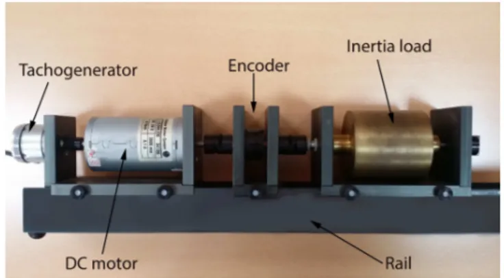
The validation of the proposed control methods is per-formed by using the modular servo system (Inteco, 2011) shown in Figure2. The objective is to control the angular position of the DC motor shaft. The system consists of the following components: a tachogenerator, a DC motor, an encoder and an inertia load. This mod-ular experimental setup supports real-time design and implementation of advanced control algorithms, and is interfaced with the MATLAB/Simulink using specific RT-DAC4/USB board for transferring the measured signals from the tachogenerator and encoder, and the control signals to the power interface unit. The angu-lar position θ of the DC motor shaft is measured by the incremental encoder, and the angular velocityω is

Figure 2: DC servo system setup

proportional to the voltage produced by the tachogen-erator. The DC motor is controlled by a PWM signal with the scaled input voltage

U(t) =V(t)/Vmax (64)

where|U(t)| ≤1 andVmax= 12[V].

In order to identify the model of the system, the iden-tification tool within Modular Servo Toolbox, which operates directly in the MATLAB/Simulink environ-ment, is used. The identification procedure is also given in (Inteco, 2011). The following transfer func-tion is obtained

G(s) = θ(s)

u(s) =

Ks

s(Tss+ 1)

(65) whereKs= 184.73 andTs= 1.3s.

By denoting x1 = θ and x2 = ω, the state space model of servo system is

˙

x1 = x2 (66)

˙

x2 = ax2+bu+w

wherea=−1/Tsandb=Ks/Ts, andwrepresents the

Coulomb friction defined by

w=Fcsign(x2) (67)

treated as the unmodeled disturbance.

The sampling period is set to T = 0.01s, and the discrete-time state space model is given by

xk+1 = Axk+Buk+Ewk (68)

yk = Cxk

with

A =

1 0.01 0 0.9923

(69)

B =

0.0071 1.4155

E =

0 1

C =

The weight matrices are chosen as

Q=

50 0 0 1

(70)

R= 1000 (71)

and the prediction horizon ofN= 20 is considered. The dynamics described by eq. (68) is split into the nominal one, eq. (7), and the deviation from the nominal, eq. (8).

Three sets of the digital simulations and real-time experiments are conducted in order to validate the pro-posed Tube MPC control methods. The reference sig-nal is defined by

r=







0 if Time steps<50 40 if 50≤Time steps≤500

0 if Time steps>500

(72)

In all three sets, the nominal MPC, v, is calcu-lated by the nominal model only, and SMC,ν, is used as the auxiliary controller to eliminate the disturbance.

A. Nominal MPC

In order to show the system response, when only the nominal MPC is applied, the first set of the digital simulation and real-time experiment is conducted. The following control

−1≤u≤1 (73)

and the state

−50≤x1≤50 (74)

−34≤x2≤34

0 200 400 600 800 1000

−10 0 10 20 30 40 50

Time steps

Angular position [rad]

r x₁ z₁

Figure 3: The angular position z1 of the nominal model, andx1 of the real plant for the nom-inal MPC

0 200 400 600 800 1000

−40 −30 −20 −10 0 10 20 30 40

Time steps

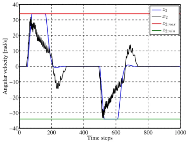
Angular velocity [rad/s]

z₂ x₂ z₂max z₂min

Figure 4: The angular velocity z2 of the nominal model, andx2 of the real plant for the nom-inal MPC

0 200 400 600 800 1000

−1 −0.8 −0.6 −0.4 −0.2 0 0.2 0.4 0.6 0.8 1

Time steps

Nominal MPC [−1,1]

v

vmax

vmin

Figure 5: Nominal MPC signal

constraints are defined.

Initially, the nominal MPC, shown in Figure 5, is applied to the nominal model. The digital simulation results, together with the corresponding experimental results, are depicted in Figures 3and 4.

It is shown that both nominal and real states respect the constraints defined by eq. (74), but there is discrepancy between the responses of the nominal model and real plant. This demonstrates the lack of robustness of the nominal MPC when it is applied to the real-time DC servo system in the presence of disturbance.

B. Tube MPC with traditional SMC

constrained separately.

The constraints for the nominal MPC and SMC are defined by

−0.7≤vk≤0.7 (75)

−0.3≤νk≤0.3 (76)

which satisfy eq. (73), i.e. −1≤v+ν ≤1. The new state constraints are calculated by using the tighten-ing procedure described in Section 4. The tightened state constraints used for the nominal system are now defined by

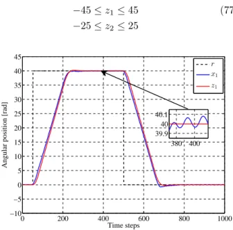
−45≤z1≤45 (77)

−25≤z2≤25

0 200 400 600 800 1000

−10 −5 0 5 10 15 20 25 30 35 40 45

Time steps

Angular position [rad]

r x₁ z₁

380 400 39.9

40 40.1

Figure 6: The angular positionz1of the nominal model for the nominal MPC, andx1of the real plant for the proposed control

0 200 400 600 800 1000

−40 −30 −20 −10 0 10 20 30 40

Time steps

Angular velocity [rad/s]

x 2 z

2 x

2max z₂max z

2min x₂min

Figure 7: The angular velocityz2of the nominal model for the nominal MPC , and x2 of the real plant for the proposed control

and the real system has to satisfy constraints defined by eq. (74). First, the digital simulation is performed, where nominal MPC signal is applied to the nominal model. Obtained results are shown in Figures 6 and 7. It can be seen that the nominal states respect constraints defined by eq. (77). The nominal MPC signal also respects the constraints defined by eq. (75), which is illustrated in Figure 8. Then, the Tube MPC with the traditional auxiliary SMC is applied to the real-time DC servo system in order to eliminate the disturbance. The parameters of the SMC component are ∆u= 0.3 andK= [−0.0118−0.0071].

The real-time system responses are also presented in Figures 6 and 7. In Figure 9 is presented the SMC component of the Tube MPC. Comparing the previous two experimental results, it is shown that the distur-bance is rejected, but there is a little chattering in the

0 200 400 600 800 1000

−0.8 −0.6 −0.4 −0.2 0 0.2 0.4 0.6 0.8

Time steps

Nominal MCP [−0.7,0.7]

v vmax

vmin

Figure 8: Nominal MPC component of the proposed control

0 200 400 600 800 1000

−0.3 −0.2 −0.1 0 0.1 0.2 0.3

Time steps

SMC [−0.3,0.3]

ν νmax

νmin

output signal. The next experiment demonstrates how to eliminate the chattering phenomenon.

C. Tube MPC with chattering free SMC

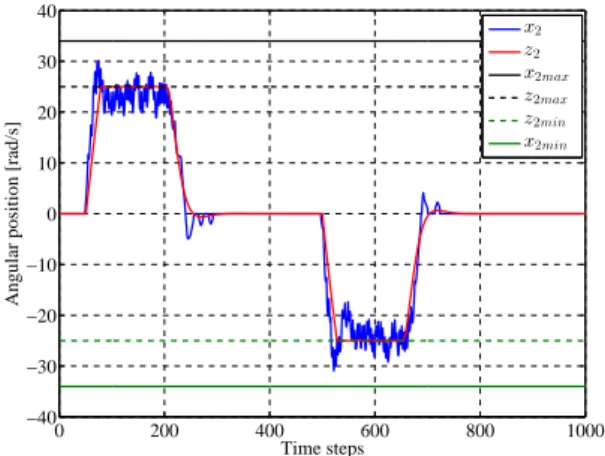
The same control and state constraints, defined by eqs. (75), (76) and (77), respectively, are used herein. The nominal MPC is applied to the nominal model first. The obtained nominal and real-time system re-sponses are illustrated in Figures 10 and 11. After that, the Tube based MPC with the chattering free SMC is applied to the real DC servo system. The SMC component is defined by eq. (20) and the parameters are ∆u = 0.3 and K = [−0.0118−0.0071]. Figure

10 shows that the chattering is eliminated. The os-cillations in SMC component between 0 and 200, as well as 500 and 700 time steps in Figure 13

origi-0 200 400 600 800 1000

−10 −5 0 5 10 15 20 25 30 35 40 45

Time steps

Angular position [rad]

380 400 39.9

40 40.1

r x₁ z₁

Figure 10: The angular position z1 of the nominal model for the nominal MPC, and x1 of the real plant for the proposed control

0 200 400 600 800 1000

−40 −30 −20 −10 0 10 20 30 40

Time steps

Angular position [rad/s]

x₂ z₂ x

2max z₂max z

2min x₂min

Figure 11: The angular velocity z2 of the nominal model for the nominal MPC, and x2 of the real plant for the proposed control

0 200 400 600 800 1000

−0.8 −0.6 −0.4 −0.2 0 0.2 0.4 0.6 0.8

Time steps

Nominal MPC [−0.7,+0.7]

v v_max vmin

Figure 12: Nominal MPC component of the proposed control

0 200 400 600 800 1000

−0.3 −0.2 −0.1 0 0.1 0.2 0.3

Time steps

SMC [−0.3/0.3]

ν νmax

νmin

Figure 13: Chattering free SMC component of the pro-posed control

nate from noise existing in angular velocity signal taken from tachogenerator (Figure 11). Therefore, they are not caused by chattering phenomenon. As in the previ-ous experiments, all states and control signals respect the defined constraints.

6. Conclusion

perfor-mances of the real system. Therefore, the procedures for calculating the required constraints tightening are derived for the both cases. The good characteristics of the proposed control algorithms are demonstrated by conducting several digital simulations and real-time experiments on the DC servo system.

Acknowledgments

This work is supported by Norwegian Ministry of Foreign Affairs, grant 2011/1383, under Programme for Higher Education, Research and Development (HERD), project NORBAS, that is leaded by Norwe-gian University of Science and Technology.

Appendix A

Proof of Theorem

3.1

The vector sequence (gk, gk+1, . . . , gk+i, . . .) , denoted

by (gk+i), converges point-wise to the limit g ∈ Rnu

if each element ofgk+i converges to the corresponding

element in g. In other words, (gk+i) is convergent if

limgk+i = g, i.e. if for every real vector ǫ >0 there

exists the natural numberNu(ǫ), such that

|gk+i−g|< ǫ, ∀i > Nu(ǫ) (A.1)

(gk+i) is the positive (negative) vector sequence if

gk+i ≥0(gk+i ≤0) fori = 0,1,2, . . .. For

multiple-input systems, it is probable that the elements of vector

gk have different signs, as they represent the switching

functions of SMC inputs. After splitting the vector gk

onto two sub vectors g_k+ andg−

k with separated

posi-tive and negaposi-tive elements ofgk, respectively, eq. (17)

can be rewritten as

g+_k+i+1=g_k+_+i−∆+

usign(g

+

k+i) + (KE)

+_w+

k+i (A.2)

g−

k+i+1=g

−

k+i−∆

−

usign(gk−+i) + (KE)

−_w−

k+i (A.3)

where ∆+

u , ∆−u ,(KE)+ ,(KE)− ,w

+

k+i andw

−

k+i are

diagonal matrices and sub vectors obtained from ∆u ,

KE and wk+i by extraction. Similarly, the theorem’s

condition given in eq. (18) can be expressed by

∆+_u1>Ω+> max|(KE)+w_k+| (A.4)

∆−

u1>Ω−> max|(KE)−w

−

k| (A.5)

and the domainGdefined by eq. (19) as

G=G+∪G− _(A.6)

with

G+={g+_k+i :|g_k+_+i|<∆+_u1 + Ω+} (A.7)

G−_={g−

k+i:|g

−

k+i|<∆

−

u1 + Ω−} (A.8)

It is obvious that (g+_k+i) and (g−

k+i), defined by eq.

(A.2), are positive and negative sequences, respectively. Let us prove now that (g+_k+i) enters the domainG+ in finite time fork0≤i≤N and remains in that area. The proof is similar in the case of (g_k−_+i) with respect toG−_{. If eq. (A.4) is true, then}

g+_k+i+1−g+k+i = −∆

+

usign(g+k+i) + (KE)

+_w+

k+i

< −∆+u1 + Ω+<0 (A.9)

and g+_k+i+1 < g_k+_+i so there exists a positive

di-agonal matrix Qk+i = diag{qk1+i q2k+i . . . q n+

u

k+i},

(0 < q_kj_+i < 1, j = 1,2, . . . , n+

u, n+u +n−u = nu) such

that

g_k+_+i+1=Qk+igk++i, Qk+i< I (A.10)

whereg_k+_+i andg−

k+i+p (p∈N) can be written as

g+_k+i =

k+i−1

Y

j=k

Qj

!

g+_k (A.11)

g_k+_+i+p =

k+i+p−1

Y

j=k

Qj

!

g_k+ (A.12)

giving the following inequality (ǫ >0₎

|g_k+_+i+p−g+_k+i|

=

k+i−1

Y

j=k

Qj

! k+i+p−1

Y

l=k+i

Ql

!

−I !

g+_k

< ǫ (A.13) According to Cauchy‘s theorem, the convergence of vector sequence (gk+i), satisfying eq. (A.13), is proved.

Its convergence domain is

G+={g_k+_+i:|g+_k+i|>∆+u1 + Ω+} (A.14)

directly satisfying eq. (A.10).

Let us now show that system trajectory enters the domain G+ _{in finite time. The sequence (g}+

k+i)

converges inside domain G+, so it is limited and lim

i→∞g

+

k+i = g

+

∞ . Assume that g+k > ∆

+

u1 + Ω+ .

According to eq. (A.2)

g+_k+i =g_k+−

k+i−1

X

j=0

(∆+u1−(KE)+wk++j). (A.15)

Suppose that g+_k+i never enters the domain G+_{. For}

i→ ∞, we obtain

∞ X

j=0

Equation (A.16) implies that the vector series

∞ X

j=0

(∆+_u1−(KE)+w+_k+j)

is convergent, and its general element ∆+

u1 −

(KE)+_w+

k+j converges to zero asj→ ∞, i.e.

∆+u1 = lim

j→∞ (KE)

+_w+

k+j

(A.17) that contradicts eq. (A.4), and the initial assumption that g_k+_+i never enters the domain G+ _{is false.} More-over, g+_k+i enters the domain G+ _{at time instant k}

0 which is bounded by the maximal element of vector

k0=int

(∆+u1−Ω+)I

−1

|g+_k| −∆+u1−Ω+

+ 1 (A.18) It is obvious that the length of the prediction horizon

Nshould be greater thank0and selected in accordance with eq. (A.18).

We will now show that for everyk0 < i < N, g_k+_+i remains in the domainG+_{. Lets}

k+k0 ∈G

+

+ ={g+k+i :

0< g+_k+i<∆+

u1 + Ω+}. Then, according to eq. (A.2),

we have

−∆+u1−Ω+ <

(A.4) −∆ +

u1 + (KE)+w+k+k0 (A.19) <

(A.4) g +

k+k0−∆

+

u1 + (KE)+wk++k0

= g_k+_+k0+1 <

(A.4)2Ω

+ _<∆+

u1 + Ω+

and thus g_k+_+i does not leave the domain G+_{. This is} also true when g_k+_+k

0 ∈G

+

− = {g

+

k+i :−∆

+

u1−Ω+ <

g_k+_+i<0} since

−∆+u1−Ω+ <

(A.4) −2Ω

+ _(A.20)

<

(A.4) −Ω

+_{+ (KE)}+_w+

k+k0 <

(A.4) −∆ +

u1−Ω++ ∆+u1

+ (KE)+w+_k+k0 <

(A.4) g +

k+k0+1=g

+

k+k0+ ∆

+

u1

+ (KE)+w+_k+k0 <

(A.4) ∆ +

u1 + Ω+

The case g+_k+k0+1 < 0 and g_k+_+k0+1 ∈/ G+ _{for g}+

k,

g_k++k0 >∆

+

u1 + Ω+ is not possible since

g_k+_+k0+1 = g_k+_+k0−∆+_u1 (A.21) + (KE)+w+_k+k0

> Ω++ (KE)+w+_k+k0>0.

Similarly, the case g_k+_+k0+1 >0 and g+_k+k0+1 ∈/ G+ forg+_k, g+_k+k

0 <−∆

+

u1−Ω+ cannot happen as

g_k++k0+1 = g

+

k+k0+ ∆

+

u1 (A.22)

+ (KE)+_w+

k+k0

< −Ω++ (KE)+w_k+_+k

0 <0.

Therefore, we have proven thatg_k+_+k

0+1∈G

+ _{and, by} induction, the latter can be generalized to

g_k+_+k0+m∈G+, (A.23) for every m > 0. The sign of gk may change at each

time step, causing the chattering in that way, but gk

will stay inG+_{. Having demonstrated that eq. (A.23)} is satisfied if eq. (A.4) is valid, the proof ends.

Appendix B

Proof of Theorem

3.2

Assume that gk ∈/ G. Then, eq. (22) becomes eq.

(17) and the proof is similar to the one discussed in Appendix A. This means that gk+k0 ∈ G where k0

is determined by eq. (A.18). Let gj_k be the jth

el-ement of gk and assume that corresponding element

(KEwk+k0)

j_{<0 . Then}

gj_k+k0+1 = g_kj_+k0−δju− |(KEwk+k0)

j_{| (B.1)}

< Ωj− |(KEwk+k0)

j_|

< δj

u− |(KEwk+k0)

j_|

< δju

where δj

u and Ωj are the jth elements in the diagonal

of ∆u and in vector Ω, respectively . Then, from eqs.

(B.1) and (22) we have

gj_k+k0+1= (KEwk+k0)

j _∈Gj _(B.2)

If (KEwk+k0)

j _{> 0, g}j

k+i will continue to decrease

and, afterk1 time instants

k1=int (δju+ Ωj

−1

(δuj−Ωj)

+ 1 (B.3)

g_kj_+k0+k1∈ {g_kj_+i:−δj

u−Ωj < g

j

k+i <0}and

g_kj+k0+k1+1 = g

j

k+k0+k1+δ

j

u (B.4)

+ |(KEwk+k0+k1)

j_|

> −Ωj_+|(KEw

k+k0+k1)

j_|

> −δj

u+|(KEwk+k0+k1)

j_|

Meanwhile, ifKEwi<0 for some i > k+k0 then eqs. (B.1) and (B.2) stand. It is implied by eqs. (B.4) and (22) that, fromi=k0+k1

gj_k+k

0+k1+1= (KEwk+k0+k1)

j_∈Gj _(B.5)

From eqs. (B.2) and (B.5) we have that oncegk enters

G, it will stay in it, i.e.

gk+i+1=KEwk+i∈G (B.6)

and, therefore, there is no chattering in sliding mode.

References

Bemporad, A. and Morari, M. Control of systems in-tegrating logic, dynamics, and constraints. Auto-matica, 1999. 35(3):407 – 427. doi:10.1016/S0005-1098(98)00178-2.

Bemporad, A., Morari, M., Dua, V., and Pistikopou-los, E. N. The explicit linear quadratic regulator for constrained systems. Automatica, 2002. 38:3–20. doi:10.1016/S0005-1098(01)00174-1.

Benattia, S. E., Tebbani, S., and Dumur, D. Hier-archical control strategy based on robust mpc and integral sliding mode - application to a continuous photobioreactor. InProceedings of 5th IFAC Confer-ence on Nonlinear Model Predictive Control. pages 212–217, 2015. doi:10.1016/j.ifacol.2015.11.285. Corradini, M. L. and Orlando, G. A vsc

algo-rithm based on generalized predictive control. Au-tomatica, 1997. 33(5):927–932. doi:10.1016/S0005-1098(96)00229-4.

Furuta, K. Sliding mode control of a discrete sys-tem. Systems & Control Letters, 1990. 14(2):145– 152. doi:10.1016/0167-6911(90)90030-X.

Garcia-Gabin, W., Zambrano, D., and Cama-cho, E. F. Sliding mode predictive con-trol of a solar air conditioning plant.

Con-trol Engineering Practice, 2009. 17(6):652–663.

doi:10.1016/j.conengprac.2008.10.015.

Golo, G. and Milosavljevi´c, C. Robust discrete-time chattering free sliding mode control.Systems & Con-trol Letters, 2000. 41(1):19–28. doi:10.1016/S0167-6911(00)00033-5.

Incremona, G. P., Ferrara, A., and Magni, L. Hi-erarchical model predictive/sliding mode control of nonlinear constrained uncertain systems. In

Proceedings of 5th IFAC Conference on Nonlin-ear Model Predictive Control. pages 102–109, 2015. doi:10.1016/j.ifacol.2015.11.268.

Inteco. Modular Servo System - Manual. Inteco, 2011. Mignone, D. The REALLY BIG Collec-tion of Logic Propositions and Linear In-equalities. Technical report, 2001. URL http://control.ee.ethz.ch/index.cgi?action= details;id=377;page=publications.

Milosavljevi´c, C. General conditions for the existence of a quasisliding mode on the switching hyperplane in discrete variable structure systems. Automation and Remote Control, 1985. 46(3):307–314.

Milosavljevi´c, C. Discrete-time vss. In A. Sa-banovi´c, L. Fridman, and S. Spurgeon, editors, Vari-able Structure Systems: from Principles to Imple-mentation, chapter 5, pages 99–128. The Institu-tion of Engineering and Technology, London, 2004. doi:10.1049/PBCE066E.

Miti´c, D., Spasi´c, M., Hovd, M., and Anti´c, D. An ap-proach to design of sliding mode based generalized predictive control. InProceedings of IEEE 8th Inter-national Symposium on Applied Computational In-telligence and Informatics (SACI) 2013. pages 347– 351, 2013. doi:10.1109/SACI.2013.6608996.

Neelakantan, V. A. Modeling, design, testing and con-trol of a two-stage actuation mechanism using piezo-electric actuators for automotive applications. Ph.D. thesis, Ohio State University, Department of Me-chanical Engineering, 2005.

Qin, S. J. and Badgwell, T. A. A survey of in-dustrial model predictive control technology.

Con-trol Engineering Practice, 2003. pages 733–764.

doi:10.1016/S0967-0661(02)00186-7.

Rakovi´c, S. V., Kerrigan, E. C., Kouramas, K. I., and Mayne, D. Q. Invariant approximations of the mini-mal robustly positively invariant sets. IEEE

Trans-actions on Automatic Control, 2005. pages 406 –

410. doi:10.1109/TAC.2005.843854.

Rawlings, J. B. and Mayne, D. Q. Model Predictive Control: Theory and Design. Nob Hill Publishing, Madison, Wisconsin, USA, 2009.

Rubagotti, M., Castanos, F., Ferrara, A., and Fridman, L. Integral sliding mode control for nonlinear sys-tems with matched and unmatched perturbations.

IEEE Transactions on Automatic Control, 2011.

56(11):2699–2704. doi:10.1109/TAC.2011.2159420. Su, W.-C., Drakunov, S. V., and Ozguner, U. An o(t2)

Utkin, V. I. Sliding Modes and Their Applications in

Variable Structure Systems. MIR, Moscow, USSR,

1978.

Young, K. D., Utkin, V. I., and ¨Ozg¨uner, U. A con-trol engineer’s guide to sliding mode concon-trol. IEEE Transactions on Control Systems Technology, 1999.

Transactions on Control Systems Technology, 1999. 7(3):328–342. doi:10.1109/87.761053.