Abstract—This paper presents a neural network global PID-sliding mode control method for the tracking control of robot manipulators with bounded uncertainties.A certain sliding mode controller with PID sliding function is developed. In this controller, the switching gain is tuned by a single-input radial-basis-function neural network on the reachable condition of sliding mode. Thus, the effect of chattering can be alleviated. Moreover, global sliding mode is realized by designing an exponential dynamic sliding function. Mathematical proof of the stability and convergence of the control system is given. Simulation results demonstrate that the chattering and the steady state errors are eliminated and satisfactory trajectory tracking is achieved.
Index Terms—Neural network, Robot, Robustness, Sliding mode control.
I. INTRODUCTION
A well known approach to the control of uncertain systems by nonlinear feedback laws is the sliding mode control [1]-[3]. Sliding mode controller design provides a systematic approach to the problem of maintaining stability in the face of modeling imprecision and uncertainty. However, chattering problem is a major drawback of sliding mode control. The boundary layer is used to avoid chattering phenomena [4]. The cost of this technology is a reduction in the accuracy of the tracking performance [5, 6].
In general, sliding mode control has two phases in the control process. One is the reaching mode, and the other is the sliding mode. The former is the phase of initial states toward the sliding surface. When the system trajectory stays on the sliding surface, the control system can reject uncertainties and disturbances. However, robust tracking is guaranteed only after the system states reach the sliding surface, and therefore robustness is not guaranteed during the reaching phase. In order to overcome this problem, some researches have been proposed, such as global sliding mode control [7-9]. Here, global sliding mode is realized by designing an exponential dynamic sliding function. In [10]-[12], the sliding mode control with PID
This work was supported in part by National Science Council, Taiwan, for financially supporting this work under Contract NSC95-2221-E-231-013.
T. C. Kuo is with the Department of Electrical Engineering, Ching Yun University, Chungli, Taiwan (phone: +886-34581196; fax: +886-34594937;e-mail: [email protected]).
Y. J. Huang is with the Department of Electrical Engineering, Yuan-Ze University, Chungli, Taiwan (e-mail: [email protected]).
sliding surface for robot manipulators were presented. Simulation results demonstrated that PID sliding surface provided faster response than that of traditional PD-manifold controller.
In this paper, a robust neural network global sliding mode PID-controller is proposed to control a robot manipulator with parameter variations and external disturbances. The chattering phenomenon is eliminated by substituting a single-input radial-basis-function (RBF) neural network. Moreover, a theoretical proof of the stability and the convergence of the proposed scheme are provided.
II. ROBOT MANIPULATOR MODEL
A. Dynamics of the Robot Manipulator
Consider an n-link robot manipulator, which takes into account the friction forces and disturbances, with the equation of motion given by [13],
τ
= + +
+C q q q G q Td q
q
M( )&& ( ,&)& ( ) , (1) where q∈Rn is the joint angular position vector of the robot
manipulator; n R
∈
τ is the applied joint torques; n n R q
M( )∈ ×
is the inertia matrix; n n R q q
C( ,&)∈ × is the effect of Coriolis and
centrifugal forces; G(q)∈Rn is the gravitational torques; and n
d R
T ∈ is the vector of generalized input due to disturbances.
B. Properties of the Robot Manipulator
Property 1. The inertia matrix M(q) is symmetric and
positive definite and satisfies
n
n M q mI
I
m1 ≤ ( )≤ 2 , ∀q∈Rn, (2)
where m1 and m2 are positive constant, and In Rn n ×
∈ is the identity matrix.
Property 2. The Coriolis and centrifugal matrix C(q,q&) satisfies
q q q
C( ,&) ≤ζc , ∀q,q&∈Rn, (3)
where ζc is a positive constant, and )(⋅ is the Euclidean
norm.
Global Stabilization of Robot Control with
Neural Network and Sliding Mode
Property 3. The gravity term is bounded as
b g q
G( ) ≤ , ∀q∈Rn, (4)
where gb is a known positive function of q.
Property 4. Using a proper definition of the matrix C(q,q&), the M&(q)−2C(q,q&) is skew-symmetric and satisfies
[
M(q)−2C(q,q)]
x=0xT & & , n R x∈
∀ . (5)
III. NEURAL NETWORK GLOBAL SLIDING MODE CONTROLLER
A. Definition of Sliding Function
Let the tracking error vector be
d q q
e= − , n
R
e∈ , (6)
where qd is the desired trajectory. The sliding function is defined as
) ( )
(
0 2
1e edt t
e
t t β
σ =&+Λ +Λ
∫
− , (7)where Λ1 and Λ2 are constant positive definite diagonal matrices. Now we define β(t) as β(t)=σ(0)exp(−αt), where
0 >
α and σ(0) is the initial value of sliding function. The choice of β(t) should satisfy: (1) β(0)=e&(0)+Λ1e(0), (2)
0 ) (t →
β as t→∞, and (3) β&(t) exits and is bounded. Notably, the function β(t) drives system states in any state space directly to the sliding mode without a reaching phase. In other words, the system states are initially located in the sliding mode. If system states are maintained on the surface for t>0, then e approaches zero and q→qd
.
The follow sliding condition will be used to develop the control law,
[
( )]
02 1
<
σ
σ M q
dt
d T . (8)
Equation (8) means that the distance to the sliding surface decreases to zero eventually along with all system trajectories. Thus, the system states are driven to the sliding surface on which sliding mode takes place.
B. Definition of Control Input
Let the subscript “o” stand for the nominal value, and symbol “ Δ ” stand for the uncertain value, i.e., M =Mo+ΔM ,
C C
C= o+Δ , G=Go+ΔG.
Assumption 1. The uncertainties of the n-link robot
manipulator (1) can be lumped asΔf ,
) (
) (
0 2 1 2
1e e q C q e edt
M f
t
d
d −Δ −Λ −Λ
∫
− Λ + Λ Δ =
Δ & && &
d T
G−
Δ −
+β& . (9)
The control input of conventional sliding mode control consists of a continuous nominal control part, and a discontinuous switching control part. The switching control part causes the chattering problem. Here we propose a single-input RBF neural network to find a suitable gain matrix to replace the switching control input.
Define the sliding mode control law as follows, based on equivalent control,
) (
) (
0 2 1 2
1 +Λ − + + −Λ −Λ
∫
Λ−
= Mo e& e &q&d β& Co q&d e tedt τ
K A
Go− −
+ σ . (10)
where
[
a a an]
diag
A= 1 2 L ,
a
i is positive constant, (11)[
k k kn]
K= 1 2 L , k ( i)
T k
i Wi i
k = Φ σ . (12)
The gain matrix K is obtained by single-input RBF neural network. The symbol
i
k
W is the m×1 vector of output layer
weights, m is the number of nodes in hidden layer, and
[
m]
Tk k
k i
ki σ φi φi L φi
2 1 )
( =
Φ is the m×1 vector of outputs
of hidden layer nodes. They can be chosen as Gaussian-type function,
) 2 / exp(
)
( 2 j2
i j i i i
i j
ki σ γ σ μ υ
φ = − − , (13)
where j i μ and j
i
υ are the center and variance of the jth basis function of the ith RBF neural network. The gain γi is a positive constant.
Define id
k
W is the ideal value of i
k
W , so that )
( i
k T k
i Wid i
k = Φ σ is the optimal compensation for Δfi, where
i f
Δ is the ith row of Δf . According to the property of universal approximation of RBF neural network, there exists
0 >
i
δ and the following condition satisfied,
i i k T k
i Wid i
f − Φ σ ≤δ
Δ ( ) , (14)
where δi is positive and can be chosen small.
C. Stability Proof
Theorem 1. Consider an n-link robot manipulator, as
described in (1), which contains unknown but bounded uncertainties. If (1) is controlled applying the control input (10) to (13), then the control system (1) is globally stable.
Proof. Choose the Lyapunov function candidate as )
( ) ( ) ( 2 1 )
(t t M q t
V = σT σ
. (15)
σ σ
σ
σ ( )
2 1 ) ( )
(t M q M q
V& = T &+ T &
. (16)
Using Property 4 and Assumption 1 and substituting controllaw (10) to (12) and Gaussian-type function (13), then Eq. (16) becomes
) (t
V&
∑
∑
[
]
= = Φ − Δ + − = n i i k T k i i n i ii f Wid i
a
1 1
2 σ (σ )
σ
∑
∑
= = Φ − Δ + − ≤ n i i k T k i i n i ii f Wid i
a
1 1
2 σ (σ )
σ
. (17)
Form the property of universal approximation of RBF neural network, assume i i i i k T k
i Wid i
f − Φ σ ≤δ ≤ρ σ
Δ ( ) , (18)
where 10<ρi< . Then, the second term on the right side of (17) satisfies
2 ) ( i i i
k T k i
i f Wid i σ ρσ
σ Δ − Φ ≤
. (19)
Therefore, one can get
∑
∑
= = + − ≤ n i i i n i i i a t V 1 2 1 2 )( σ ρσ
& . (20)
Since
a
i is a positive constant and ai >ρi is chosen, it is clear that0 ) (t ≤
V& . (21) Equation (21) guarantees the decay of the energy of σ as long
as σ ≠0. Thus, the overall system is stable.
█
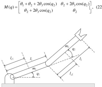
IV. EXAMPLE AND SIMULATION RESULTS
Consider a two-link robot manipulator [14] as shown in Fig. 1. The parameter matrices are as follows:
⎥ ⎦ ⎤ ⎢ ⎣ ⎡ + + + + = 2 2 3 2 2 3 2 2 3 2 1 ) cos( 2 ) cos( 2 ) cos( 2 ) ( θ θ θ θ θ θ θ θ q q q q
M , (22)
Fig. 1. Two-link robot manipulator
⎥ ⎦ ⎤ ⎢ ⎣ ⎡− − + = 0 ) sin( ) )( sin( ) sin( ) , ( 1 2 3 2 1 2 3 2 2 3 q q q q q q q q q C & & & & & θ θ θ , (23) ⎥ ⎦ ⎤ ⎢ ⎣ ⎡ + + + + = ) cos( ) cos( ) cos( ) ( ) ( 2 1 6 2 1 6 1 5 4 q q g q q g q g q G θ θ θ θ , (24)
where g is the gravitational acceleration and 1 2 1 2 2 1 1
1=mlc +ml +I
θ , (25)
2 2
2 2 2=mlc +I
θ , (26)
2 1 2 3 =mllc
θ , (27)
1 1 4=mlc
θ , (28)
1 2 5 =ml
θ , (29)
2 2 6=mlc
θ . (30)
Assume that the parameters of the unloaded robot are given by Table 1. The desired trajectories are
⎥ ⎦ ⎤ ⎢ ⎣ ⎡ − − − − − − − − = ⎥ ⎦ ⎤ ⎢ ⎣ ⎡ = ) 8 exp( 8 . 12 ) 8 exp( 6 . 1 6 . 1 ) 8 exp( 8 . 12 ) 8 exp( 6 . 1 6 . 1 2 1 t t t t t t q q q d d
d . (31)
Regarding an unknown load carried by the robot as part of the second link, the parameters m2 , lc2 and I2 change to
2
2 m
mO+Δ , lc2O+Δlc2 , and I2O+ΔI2 , respectively. Suppose that the variation of parameters lies in the intervals:
3
0≤Δm2≤ , 250≤Δlc2≤0. , and 0≤ΔI2≤0.5 . The external disturbance is assumed to be
⎥ ⎦ ⎤ ⎢ ⎣ ⎡ + + = ) 02 . 0 sin( 7 . 1 5 . 3 ) 02 . 0 cos( 2 2 . 3 t t
Td . (32)
In order to achieve that the desired response of each joint of the manipulator being a second-order critically damped response, we choose damping ratio to be 1 and natural frequency to be 13 rad/sec. Therefore, the sliding function
constants are ⎥
⎦ ⎤ ⎢ ⎣ ⎡ = Λ 26 0 0 26
1 and ⎥
⎦ ⎤ ⎢ ⎣ ⎡ = Λ 169 0 0 169
2
.
Thecontrol input is chosen as in (10) to (13). The matrix A is ⎥ ⎦ ⎤ ⎢ ⎣ ⎡ = 50 0 0 50
A . The gains of Gaussian-type function are
18 1=
γ and γ2=12.
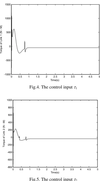
The simulation results are shown in Figs. 2 to 5. Figs. 2 and 3 show that both q1 and q2 converge to the desired trajectories. From Figs. 4 and 5, it is obvious that chattering of the control input is eliminated by applying the proposed method.
Table 1. Parameters of the robot manipulator
m1 m2o l1 l2o lc1 lc2o I1 I2o
0 0.5 1 1.5 2 2.5 3 3.5 4 4.5 5 0
0.2 0.4 0.6 0.8 1 1.2 1.4 1.6 1.8 2
Time(s)
J
oi
nt
an
gl
e
1
(R
a
d)
q1 qd1
Fig. 2. The response of q1 and desired path q1d
0 0.5 1 1.5 2 2.5 3 3.5 4 4.5 5
0 0.2 0.4 0.6 0.8 1 1.2 1.4 1.6 1.8 2
Time(s)
J
oi
nt
angl
e 2
(
R
ad
)
q2 qd2
Fig. 3. The response of q2 and desired path q2d
V. CONCLUSION
In this paper, a robust neural network global sliding mode PID-controller is proposed to control a robot manipulator with parameter variations and external disturbances. In classical sliding mode control, the control input gain is chosen to be lager than the bound of the uncertainties, which means the controller has to have a prior knowledge of the uncertainties. The proposed method can compensate the uncertainties. The common problem of input chattering is also eliminated and hence the control input is smooth. The other advantage of the proposed method is that it possesses sliding mode characteristics all the time without a reaching phase.
REFERENCES
[1] V. I. Utkin, Sliding Mode in Control and Optimization. New York: Springer-Verlag, 1992.
[2] J. Y. Hung, W. Gao, and J. C. Hung, “Variable structure control: a survey,” IEEE Trans. Ind. Electr., vol. 40, 1993, pp. 2-22.
0 0.5 1 1.5 2 2.5 3 3.5 4 4.5 5
-1000 -500 0 500 1000 1500
Time(s)
T
or
que
of
Li
nk
1 (
N
M
)
Fig.4. The control input τ1
0 0.5 1 1.5 2 2.5 3 3.5 4 4.5 5
-800 -600 -400 -200 0 200 400 600 800 1000
Time(s)
T
o
rque of
Li
nk
2 (
N
M
)
Fig.5. The control input τ2
[3] K. D. Young, V. I. Utkin, and Ü. Özgüner, “A control engineer's guide to sliding mode control,” IEEE Trans. Control Sys. Tech., vol. 7, 1999, pp. 328-342.
[4] J. J. E. Slotine and W. Li, Applied Nonlinear Control. New Jersy: Prentice-Hall, 1991.
[5] P. Guan, X. J. Liu, and J. Z. Liu, “Adaptive fuzzy sliding mode control for flexible satellite,” Engineering Appl. Arti Intelli., vol. 18, 2005, pp. 451-459.
[6] Y. Fang, T. W. S. Chow, X. D. Li, “Using of a recurrent neural network in discrete sliding-mode control,” Proc. Inst. Electr. Eng. Control Theory Appl., vol. 146, 1999, pp. 84-90.
[7] H. S. Choi, Y. H. Park, Y. Cho, and M. Lee, “Global sliding-mode control: improved design for a brushless DC motor,” IEEE Control Sys. Mag., vol. 21, 2001, pp. 27-35.
[8] R. J. Mantz, H. de Battista, and F. D. Bianchi, “VSS global performance improvement based on AW concept,” Automatica, vol. 41, 2005, pp. 1099-1103.
[9] Z. Wang, J. Zhang, Z. Chen, and Y. He, “Neural network_based on adaptive discrete-time global sliding mode control scheme,” Intelligent Control and Automation. Lecture Notes in Control and Information Science, New York: Springer-Verlag, Vol. 344, 2006.
[10] Y. Stepanenko, Y. Gao, and C. Y. Su, “Variable structure control of robots with PID sliding surfaces,” Int. J. Robust Nonlinear and Control, vol. 8, 1998, pp. 79-90.
[12] E. M. Jafarov, M. N. A. Parlakc, and Y. Istefanopulos, “A new variable structure PID-controller design for robot manipulators,” IEEE Trans. Control Sys. Tech., vol. 13, 2005, pp. 122-130.
[13] M. W. Spong, “On the robust control of robot manipulators,” IEEE Trans. Automa. Control, vol. 37, 1992, pp. 1782-1786.