LINEAR INVERSION OF A NEGATIVE GRAVITY ANOMALY IN SE RIO GRANDE CONE:
A GRABEN ON OCEANIC CRUST?
Emilson Pereira Leite
1and Naomi Ussami
2Recebido em 19 maio, 2006 / Aceito em 29 setembro, 2006 Received on May 19, 2006 / Accepted on September 29, 2006
ABSTRACT.We detect, for the first time, a negative free-air gravity anomaly of 23 mGal amplitude over a region in the South Atlantic Ocean centered at48◦W and 35◦S. To this end, we used the integration of conventional shipborne gravity data and gravity data derived from GEOSAT/ERM satellite altimetry. The north bound of this anomaly coincides with the Chu´ı Lineament and the south bound indicates another lineament, which is the extension of the Meteor Fracture Zone. The anomaly trend is NE-SW, its width is 400 km and its length is 600 km. Two-dimensional linear inversion with relative and absolute equality constraints was used to calculate the density distribution along three profiles perpendicular to the main axis of the anomaly. The result suggests that the sediment thickness in the deepest part of the basin is at least 3.0 km where the ocean bathymetry is 4,800 m. This tectonic feature, an asymmetric half-graben formed between two lineaments, probably lies over an oceanic crust. The estimated volume of sediments in this basin is approximately 50% of the post-Miocene sediments volume deposited in the Rio Grande Cone where gas-hydrates were found.
Keywords: Potential Methods, Gravity Inversion, Rio Grande Cone, Oceanic Crust.
RESUMO.Uma anomalia ar-livre com amplitude negativa de 23 mGal em uma regi˜ao no oceano Atlˆantico Sul, centrada em48◦W e35◦S, foi observada pela primeira vez devido `a integrac¸˜ao de dados de gravimetria marinha convencionais e dados de gravidade derivados de altimetria por sat´elite, adquiridos pela miss˜ao GEOSAT/ERM. O limite norte desta anomalia coincide com o Lineamento Chu´ı e o limite sul indica outro lineamento, que ´e uma extens˜ao da Zona de Fratura Meteoro. A anomalia tem direc¸˜ao NE-SW, sua largura ´e de 400 km e seu comprimento ´e de 600 km. Foi utilizada uma metodologia de invers˜ao linear bidimensional, com v´ınculos relativos e absolutos, para calcular a distribuic¸˜ao de densidades ao longo de trˆes perfis paralelos ao eixo principal da anomalia. O resultado sugere que a espessura de sedimentos na parte mais profunda da bacia ´e de no m´ınimo 3,0 km onde a batimetria oceˆanica ´e de 4.800 m. Esta feic¸˜ao tectˆonica, um semi-gr´aben assim´etrico formado entre dois lineamentos, provavelmente situa-se sobre uma crosta oceˆanica. O volume de sedimentos estimado para esta bacia ´e de cerca de 50% do volume de sedimentos p´os-Mioceno depositados no Rio Grande Cone, onde hidratos de g´as foram encontrados.
Palavras-chave: M´etodos potenciais, Invers˜ao gravim´etrica, Cone do Rio Grande, Crosta oceˆanica.
1Department of Geology and Natural Resources, Institute of Geosciences, State University of Campinas, 13083-970 Campinas, SP, Brazil. Postal box: 6152, Tel: (19) 3521-4697; Fax: (19) 3289-1562 – E-mail: [email protected]
INTRODUCTION
A free-air anomaly map in Southern Atlantic was obtained through integration of conventional shipborne gravity data and gravity data derived from GEOSAT/ERM satellite altimetry (Fig. 1), using the Least Squares Collocation technique (Leite et al., 1999). This technique assumes that a set of observations associated to any component of the Earths gravity field can be related to the ano-malous gravitational potential through appropriate linear functi-onals. If the covariances between such components are known, then it is possible to estimate any other component of the Earths gravity field. This allows two or more components to be integra-ted, so that the output can be any one of them for a given study area. The errors associated with the observations and with the es-timated quantities are taken into account rigorously in the Least Squares Collocation. Gravity free-air anomalies and height ano-malies are the components of the Earths gravity field that were used in the estimation of the free-air anomalies used in this study.
Figure 1– (a) Conventional shipborne gravity data; (b) satellite altimetry (GEOSAT/ERM).
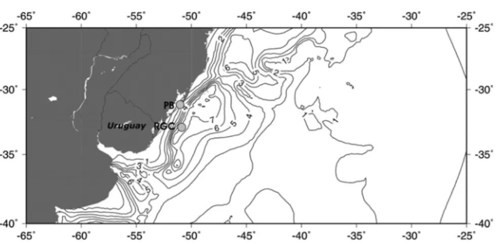
The free-air anomaly map defined a negative gravity anomaly (Fig. 2) centered at48◦W and35◦S, on the southeast border of
Rio Grande Cone (Fontana, 1992). Figure 2 also shows the main physiographic features in the region. To the authors knowledge, this anomaly has never been mapped before because it was used gravity datasets either from the conventional shipborne survey or derived from satellite altimetry (e.g. Andersen & Knudsen, 1995). This paper shows the advantage of using an integrated approach in mapping marine gravity anomalies. Figure 2 also shows the main physiographic features in the region, which are the S˜ao Paulo Plateau, the Rio Grande Rise, the Pelotas Basin, the Rio-Grandense Shield and the Rio Grande Cone.
Contrary to interactive forward modeling, an inversion method does not require a complete knowledge about the ano-malous source. Rather, an inversion method requires few prior geologic constraints which must be mathematically incorporated by the method in an automatic way. This procedure is frequently adopted to obtain a unique and stable solution in gravity interpre-tation (Silva et al., 2002).
In this study, we have been working only with constrained li-near inversion using the same idea described in Barbosa et al. (1997). The difference here is that we estimated the density con-trast distribution that fits the observed anomaly within the mea-surement errors and represents smooth spatial density variations (Barbosa et al., 2002). So, a discrete density distribution is esti-mated by standard linear inversion stabilized by imposing smooth spatial density variations. The premise of a smooth spatial density distribution is justified by smooth spatial distributions of gravity values along selected gravity anomaly profiles, i.e. high wave-number anomalies that could represent real anomalous sources within the crust are not detectable in these profiles.
In this paper, we estimate the discrete density distribution along three gravity profiles over the SE Rio Grande Cone by using an inverse technique which incorporates relative constraints and absolute equality constraints (Barbosa et al., 1997). In the inver-sions presented here, relative constraints are used to guarantee smooth spatial density variations, while equality constraints are used to set density values associated with specific cells which define the interpretation model.
Figure 2– Main physiographic features over the study region (circles): SPP – S˜ao Paulo Plateau; RGR – Rio Grande Rise; PB – Pelotas Basin; RGS – Rio-Grandense Shield; RGC – Rio Grande Cone.
RESIDUAL GRAVITY ANOMALY MODELING
The Earths Gravity Field is produced by a superposition of over-lapping gravitational effects of many sources within the crust. Local gravity anomalies associated with near surface masses are referred as to residual anomalies and gravity anomalies due to larger and deeper geological features are referred as to regional anomalies.
In order to obtain the residual anomaly of the region shown in Figure 1, firstly we calculated the gravitational effect due to bending of the crust-mantle interface in response to sedimentary loads in order to check whether this component was important on the observed anomaly.
We also removed from the observed anomaly a polynomial flat surface, which is a regional field that represents sources deeper than about 10 km.
The following sections describe how the residual gravity ano-maly was obtained.
Flexural Effect of Sedimentary Loads
Lithosphere and crust-mantle boundary is flexed due to sedi-mentary loads and this deformation produces long wavelength components on the gravity field. Thus, it is necessary to calcu-late the gravitational effect of this flexure and to remove it from the observed anomalies.
A sediment isopach map (Emery & Uchupi, 1984) based on reflection and refraction seismic, well stratigraphy, and DSDP (Deep Sea Drilling Project) data were digitized (Fig. 3).
Next to the Pelotas Basin it is possible to see a thick sedi-mentary layer centered at48◦W and32◦S with up to 7 km of
sediments. In the southern continental margin of Uruguay there is also a 7 km wedge of sediment and a thick sedimentary layer in the Rio Grande Cone is also observed.
An algorithm developed by Shiraiwa (1994) was used to estimate the gravitational effect due to the flexure of the litho-sphere caused by the sedimentary loading. In this algorithm, the lithosphere is approximated by a thin elastic plate, with a load on its top (Timoshenko & Goodier, 1970). The gravitational effect of the deformed crust-mantle boundary is calculated by Parkers method (Parker, 1972). The parameters used to calculate gravi-tational effect of this deformation are: effective elastic thickness
= 10km; sediment density= 2.4g/cm3; crust oceanic rocks
density = 2.9g/cm3; and mantle density= 3.3g/cm3.
Fi-gure 4 shows that the gravitational effect due to flexure is less than 10–1mGal, therefore lower than the error in the free-air
ano-maly estimate.
Regional-Residual Separation
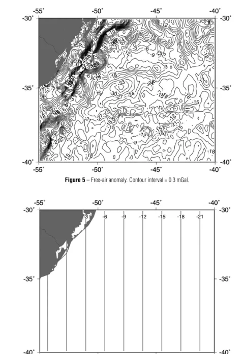
A deep source anomaly associated with variations in crust-mantle boundary and lower crust is observed and it should be removed in order to invert the anomalies associated with shallow sources. For this purpose, a first degree polynomial surface was fitted to the original gravity data (Fig. 5) in order to estimate the regio-nal gravity field. Figures 6 and 7 show the regioregio-nal and residual anomalies, respectively. Gravity profiles were extracted from the residual anomaly shown in Figure 7.
LINEAR INVERSION METHODOLOGY
The solution of gravity data inversion is neither unique nor stable. Therefore it is an ill-posed problem (Hadamard, 1902). A way to reduce the instability and to guarantee the uniqueness of the solution is to introduce a priori information about un-known parameters.
con-Figure 3– (a) Sediment isopach map from Emery & Uchupy (1984). Contour interval = 1 km.
Figure 4– Gravitational effect of crust-mantle boundary flexure due to sediment load on the Free-Air anomaly. Contour interval = 0.1 mGal.
tains several methods to calculate physical properties, which ge-nerally is density, while body geometry is fixed. These methods are used to map lateral and subsurface density distribution (e.g. Braile et al., 1974; Bear et al., 1995). Nonlinear methods are used to calculate body geometry while physical properties are fixed and these methods are useful to calculate anomalous bodys position and orientation and layers depths (e.g., Richard-son & MacInnes, 1989; Barbosa et al., 1997).
We have chosen the linear inversion because, more than the geometry of the anomalous body, we wanted to learn about the stratigraphy of the basin and how it was formed. This information should be reflected in the density distribution.
The inverse problem can be expressed as a linear system like
g =Gρ , (1)
whereGis a linear operator (usually called sensitivity matrix) that describes the relationship between unknown model parameters
(ρ)and data(g). MatrixGwill be defined using a forward method like that described in Talwani et al. (1959). To estimate
ρ we assume that a set ofM juxtaposed cells represents the medium beneath theNpoints where the datagwas collected. Let us defineρas theM-dimensional density contrast vec-tor to be estimated, andgas theN-dimensional gravity ano-maly vector produced by theMcells. We can impose the fitting of gravity data by minimizing the functional
ϕg(g0, g) = ||g0−g||2, (2)
where|| · ||is the Euclidean norm. Estimatingρfromgis a linear problem in this case. We will describe a method to estimate
ρincorporating additional constraints.
Minimizing the functional below incorporates the relative equality constraints, namely the smooth density variation cons-traints
ϕx(ρ) = fr||Rρ|| 2
Figure 5– Free-air anomaly. Contour interval = 0.3 mGal.
Figure 6– Regional free-air anomaly (first-order polynomial surface). Contour interval = 0.3 mGal.
where fr is a normalizing factor,Ris a matrix L×M, where Lis the number ofa priorirelationships between pairs of para-meters. if we know that the density of theithblock is twice the density of thejthblock, then theithandjthelements of the spe-cific row ofRthat corresponds to the constraint will take values 1 and 2, respectively, whereas the rest of the elements in this row will be zero, giving rise to the expressionρi −2ρj ∼= 0
(Barbosa et al., 1997). Notice that it is possible to use different relationships in the same R matrix. For example, it can establish
a linear relationship among the parameters forcing the increase of densities with depth.
Minimizing the functional below incorporates the absolute equality constraints
ϕa(ρ) = fa||Aρ−h||2, (4)
den-Figure 7– Residual free-air anomaly. Contour interval = 0.3 mGal.
sities. The term fais a normalizing factor. For instance, if theith
parameter is known and its value is 0.5, we just have to set 1.0 in theith column and first row of the matrixA, whereas the rest of the elements are set to zero. Accordingly, the first element of
hwill be 0.5.
The terms faand frare given by
fa = ||G||
||A|| and fr =
||G||
||R|| (5)
where|| · ||is the Euclidean norm.
Incorporating the constraints (3) and (4) to the problem can be done by minimizing the unconstrained functional in the least-squares sense
ϕ(ρ)=µrϕr(ρ)+µaϕa(ρ)+ϕg(g0, g). (6)
Its solution to the vectorρis
ρµafa(AtA)+GtG+µr fr(RtR)− 1
µafaAth+Gtg0.
(7)
The constantsµaandµrare weights associated to each kind
of constraints.
RESULTS OF DATA INVERSION
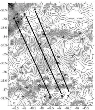
The proposed inversion methodology was applied to three gra-vity profiles shown in Figure 8: A-A, B-B and C-C. These profiles were extracted from the free-air anomaly residual map (Fig. 7).
For each profile, the interpretative subsurface model consisted of 225 cells (15×15cells with dimensions equal to 21 km and
0.35 km along x- and z- directions, respectively).
Figure 8– Residual free-air anomaly and profiles used in the inversion proce-dure. Contour interval = 3 mGal.
Absolute constraints were set as follows: the densities of the two top layers, at depths between 4.8 km and 5.5 km, were fi-xed with values of 2.4 g/cm3based on seismic results given by
considered to represent the mean density of the crustal basement in the study area. Therefore, 0.6 g/cm3was the density contrast
value set into thehvector of Equation 7. The two bottom layers, at depths between 9.2 km and 10 km, had cells fixed with va-lues of 2.9 g/cm3, which gives a density contrast of 0.1 g/cm3.
Cells constrained with absolute values are shown in Figure 9 as gray cells. Absolute constraints also helps in order to limit the range of possible values associated with the free-cells, thus bia-sing the solution towards a set of geologically sound density va-lues. The weight associated with the absolute constraints was set equal toµa=1.0.
Figure 9– Interpretative model used in the inversion procedures. The subsur-face was subdivided into 225 cells (15×15). Absolute constraints were applied to gray cells in the two top layers by setting a density value of 2.4 g/cm3and in the two bottom layers by setting a density value of 2.9 g/cm3.
Relative constraints were used in order to impose an overall smoothness on the density distribution estimate, as described in the methodology section. The weight associated with the relative constraints was set equal toµr =0.1. The combination of these
two constraints provides a density distribution that is smooth and increases with depth, as was expected given the shapes of the anomalies together with the geological knowledge of the area.
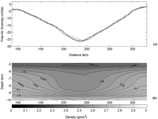
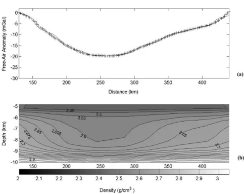
Figures 10, 11 and 12 show the inversion results of the free-air anomalies profiles, A-A’, B-B’ and C-C’, respectively. These results are consistent with a basin formation of evolution due to rifting and rapid initial subsidence. A uniform density distribution as shown in Figure 13, layer A, is expected if the first phase of sedimentation layer B refers to sedimentation well after rifting and oceanic lithosphere subsidence.
DISCUSSION
Sediment volume stored in this basin corresponds to approxi-mately 50% of after-Miocene sediment volume stored in the Rio Grande Cone where gas-hydrates were found (Fontana, 1992).
LEPLAC seismic data are not available but Russo (1999) cal-culated an isopach map for the study area and its surroundings. This map shows a sedimentary thickness of 2.5 to 3 km, which is approximately equal to the inversion results, although there is no evidence in this map for the existence of a basin associated with the sedimentary layer.
Figure 14 shows the free-air anomaly overlapped by the tec-tonic map. We can see that the north limit of the negative free-air anomaly coincides with the Chu´ı Lineament, which extends to the Mid-Ocean Atlantic Ridge. The south limit of the anomaly appe-ars to be another lineament and it is shown on the same figure, between the parallels−37◦and−36.5◦. This lineament may
represent an extension of the Meteor Fracture Zone.
The graben-like structure of this basin may be associated with a rifting event that occurred in response to adjacent continental margin uplifting (Leite, 2000) in the Eocene. This process was responsible firstly to open the graben and secondly to store the sediment, due to erosion post-uplifting.
The results of inversion, synthesized in Figure 13, also sug-gests a rapid subsidence in the rifting phase resulting in a uniform sediment storing as we can see in layer A. Post-rifting sediment storing, represented by layer B, occurred in the after-Miocene as a slower process, which results in thinner sediment layers with density lower than that found in layer A.
CONCLUSIONS
We performed a regional-residual separation on an integrated gravity map, through a first-order polynomial fitting, after which we extracted three free-air anomaly profiles across the main axis of a negative 23 mGal amplitude anomaly from the resi-dual map. This anomaly is centered at48◦W and35◦S on the South Atlantic Ocean. We then estimated density distributions using a constrained linear gravity inversion methodology.
Inversion results suggest that the thickness in the deepest part of the basin is at least 3.0 km where the ocean bathymetry is 4,800 m. At this bathymetric depth we would expect to find oceanic crust.
Figure 10– Profile A-A: Two-dimensional density distribution estimate. (a) Observed (crosses) and fitted (solid line) residual free-air anomalies. (b) Estimated density distribution. Contour interval is 0.025 g/cm3.
Figure 12– Profile C-C: Two-dimensional density distribution estimate. (a) Observed (crosses) and fitted (solid line) residual free-air anomalies. (b) Estimated density distribution. Contour interval is 0.025 g/cm3.
Figure 13– Schematic layered model inferred from inversion results. Depth and horizontal distances are not at the same scale.
ACKNOWLEDGMENTS
We thank FAPESP for the financial support (Process number: 98/00107-8). The first author is specially thankful to the Ins-titute of Astronomy, Geophysics and Atmospheric Sciences of the University of S˜ao Paulo, for all the computational, material and personal support during the time this work was carried out. We also thank Val´eria Cristina F. Barbosa for her valuable com-ments, corrections and suggestions.
REFERˆENCIAS
ANDERSEN OB & KNUDSEN P. 1995. Global altimetric gravity map from the ERS-1 geodetic mission (cycle 1). Earth Observation Quarterly, 47: 1–5.
BARBOSA VCF, MEDEIROS WE & SILVA JB. 1997. Gravity inversion of basement relief using approximate equality constraints on depths. Geophysics, 62: 1745–1757.
incorpora-Figure 14– Free-air anomaly map overlapped by tectonic structures over the study area. The E-W dotted line situated between the parallels−37◦and−36.5◦indicates a possible lineament.
tion of concrete geologic information. Geophysics, 67: 795–800.
BEAR GW, AL-SHUKRI HJ & RUDMAN AJ. 1995. Linear inversion of gravity data for 3-D density distributions. Geophysics, 60: 1354–1364.
BRAILE LW, KELLER GR & PEEPLES WJ. 1974. Inversions of gra-vity data for two-dimensional density distributions. J. Geophys. Res., 19: 2017–2021.
EMERY KO & UCHUPI E. 1984. The Geology of the Atlantic Ocean, Springer-Verlag, New York, 1050pp.
FONTANA RL. 1992. Investigac¸˜oes Geof´ısicas Preliminares Sobre o Cone do Rio Grande e Bacia de Pelotas – Brasil. Acta Geol. Leop., 13(30): 161–170.
HADAMARD J. 1902. Sur les probl`emes aux d´eriv´ees et leur signification physique: Bull Princeton Univ., 13: 1–20.
LEITE EP, MOLINA EC & USSAMI N. 1999. Integrac¸˜ao de dados de gra-vimetria marinha e de altimetria por sat´elite (GEOSAT/ERM) no Atlˆantico Sul (25/40◦S e65/25◦W). Rev. Bras. Geof´ısica, 17: 145–161.
LEITE EP. 2000. Estrutura da litosfera a partir da interpretac¸˜ao de da-dos geopotenciais na regi˜ao compreendida entre25/40◦S e25/60◦W. Dissertac¸˜ao de Mestrado. IAG/USP, S˜ao Paulo, 109 pp.
LEYDEN R, LUDWING WJ & EWING M. 1971. Structure of the conti-nental margin off Punta del Este, Uruguay, and Rio de Janeiro, Brazil. Am. Ass. Petrol. Geol., Bull. 55(12): 2161–2173.
PARKER RL. 1972. The rapid calculation of potential anomalies. Geo-phys. J. Roy Astr. Soc., 31: 447–455.
RICHARDSON RM & MACINNES SC. 1989. The inversion of gravity data into three-dimensional polyhedral models. J. Geophys. Res., 94: 7555–7562.
RUSSO LR. 1999. LEPLAC: Is´opacas de sedimentos e profundidade do embasamento na margem continental brasileira. 6◦Congresso In-ternacional da Sociedade Brasileira de Geof´ısica. Resumo expandido (CD-ROM).
SHIRAIWA S. 1994. Flexura da litosfera continental sob os Andes Cen-trais e a origem da Bacia do Pantanal, Tese de Doutoramento, Univ. de S˜ao Paulo, S˜ao Paulo, Brasil, 110 pp.
SILVA JBC, MEDEIROS WE & BARBOSA VCF. 2002. Practical applicati-ons of uniqueness theorems in gravimetry: Part I – Capplicati-onstructing sound interpretation methods. Geophysics, 67: 788–794.
TALWANI M, LAMAR WORZEL J & LANDISMAN M. 1959. Rapid Gra-vity Computations for two-dimensional bodies with application to the Mendocino Submarine Fracture Zone. J. Geophys. Res., 64(1): 49–59.
NOTES ABOUT THE AUTHORS
Emilson Pereira Leite. Collaborator Researcher at the DGRN/IG-Unicamp. He received his Master’s (2000) and Ph.D. (2005) degrees in Geophysics both from IAG/USP. His current research interests are in the area of spatial modeling and integration of geophysical and remotely sensed data and inversion methods in Geophysics.