Bol. Ciênc. Geod. vol.21 número1

http://dx.doi.org/10.1590/S1982-217020150001000012

DETERMINISTICALLY-MODIFIED INTEGRAL

ESTIMATORS OF GRAVITATIONAL TENSOR

Estimadores integrais determinísticos modificados do tensor gravitacional

MOHSEN ROMESHKANI1,*

MEHDI ESHAGH2

1_{Islamic Azad University, Qazvin branch, Qazvin, Iran}

2_{Department of Engineering Science, University West, Trollhättan, Sweden}

Email: mehdi.eshagh@hv.se

ABSTRACT

The Earth’s global gravity field modelling is an important subject in Physical

Geodesy. For this purpose different satellite gravimetry missions have been designed and launched. Satellite gravity gradiometry (SGG) is a technique to measure the second-order derivatives of the gravity field. The gravity field and steady state ocean circulation explorer (GOCE) is the first satellite mission which uses this technique

and is dedicated to recover Earth’s gravity models (EGMs) up to medium

wavelengths. The existing terrestrial gravimetric data and EGM scan be used for validation of the GOCE data prior to their use. In this research, the tensor of gravitation in the local north-oriented frame is generated using deterministically-modified integral estimators involving terrestrial data and EGMs. The paper presents that the SGG data is assessable with an accuracy of 1-2 mE in Fennoscandia using a modified integral estimatorby the Molodensky method. A degree of modification of 100 and an integration cap size of 2.5o _{for integrating 5} _{5 terrestrial data are} proper parameters for the estimator.

Keywords: Isotropic Kernels; Gravity Anomalies; Gravity Gradients; Modification;

Simulation of Gravitational Tensor; Truncation Coefficients.

RESUMO

O modelo de campo de gravidade global da Terra é um assunto importante na geodésia física. Para este propósito, diferentes missões de satélites gravimétricos têm

sido construídas e lançadas. A gravimetria da gravidade de satlite – SGG – é uma

técnica para medir os “derivativos de segunda ordem” do campo da gravidade. O campo de gravidade é a exploração da circulação do oceano em estado de equilíbrio pelo – GOCE- primeira missão com satélite que usa esta técnica e é dedicada para readquirir os modelos de gravidade da Terra – EGMs – em ondas de tamanho médio. Os dados gravimétricos terrestres existentes e os de varredura – EGM são usados para validar os dados do GOCE antes de serem usados. Nesta pesquisa, o tensor de gravitação na estrutura local orientada ao Norte argumenta que os dados SGG – gradiometria da gravidade de satélite – é acessível com uma precisão de 1 – 2 m. E em Fennoscandia usando um estimador integral modificado pelo método de Molodensky. O grau de modificação de 100 e uma integração no tamanho de 2.5°

para a integrada de 5’ x 5’ de dados terrestres são parâmetros apropriados para o estimador.

Palavras-chave: Núcleo isotrópico; da gravidade; gradiente gravitacional;

modificação; simulador de tensor gravitacional; coeficiente de truncamento.

1. INTRODUCTION

Satellite gravity gradiometry (SGG) is a space method for recovering the Earth’s gravity field from the second-order derivatives of the field. Delivering Earth’s gravity models (EGMs) with higher resolution than those recovered from former satellite gravimetry techniques is expected from these data. The gravity field and steady-state ocean circulation explorer (GOCE) mission (BALMINO et al. 1998, 2001, ESA 1999, ALBERTELLA et al. 2002, RUMMEL et al. 2002, DRINKWATER et al. 2003) was successfully launched on 17th _{March 2009 as the first satellite mission which used the}

SGG technique. So far GOCE has delivered EGMs todegree and order 250 corresponding to a resolution of 60 km by 60 km. The second-order derivatives of the gravity field is measured by a gradiometer mounted on the GOCE spacecraft and validation of them is very important prior to their use for any purpose. Having erroneous observations leads to the deviation of the recovered gravity field from the true one and wrong interpretation for the geophysical phenomena.

Numerous studies have been done in the Earth's gravity field modelling from SGG for years, but the idea of validating the SGG data was presented in a few different ways. In the following we divide the validation methods into two different categories:

a) Validation of GOCE products

(GRACE) (Tapley et al. 2005) and concluded that they do not outperform the GRACE orbit; therefore, combination of GRACE and GOCE data is useful. They found significant improvements between degrees 50 and 200 for geoid computation goal. Janak and Pitonak (2011) evaluated the GOCE products in central Europe and Slovakia. They mentioned that TIM2 and SPW2 to degree 210 are much better than the previous releases to the same degree and GOCO02S (GOIGINGER et al. 2011) has a significant improvement comparing to GOCO01S (PAIL et al. 2010). Sprlak et al. (2012) did the same study in Norway and mentioned that the direct solutions are highly affected by a priori information and time-wise solution is more reliable. Abdalla et al. (2012) evaluated the GOCE EGMs in Sudan and concluded that the SPW1, SPW2, TIM1, TIM2 and GOCO01S are consistent with the local data. Abdalla and Tenzer (2012) validated EGMs in New Zealand. Guimaraes et al. (2012) tested the EGMs in Brazil and found out that TIM3 is much better than the previous ones, as expected. Eshagh and Ebadi (2013) also investigated different EGMs and evaluated them over Fennoscandia. So far evaluation of the GOCE EGMs was done based on comparison of the EGM products with external sources of data, like gravity anomaly, disturbing gravity, geoid and/or astrogeodetic deflections. However, it should be considered that the errors of EGMs have been also presented. Wanger and McAdoo (2012) noticed that the errors of GOCE EGMs are not realistic and tried to calibrate them based on EGM08 (Pavlis et al., 2008, 2012). Eshagh (2013) studied the reliability and calibration of GOCE EGMs as well. Eshagh and Ebadi (2014) presented a method for error calibration of some GOCE EGMs based on condition adjustment models.

b) On board validation of GOCE data

Bouman et al. (2003) has set up a calibration model based on the instrument (gradiometer) characteristics to validate the SGG data. Bouman and Koop (2003) presented an along-track interpolation method to detect the outliers. Their idea is to compare the along-track interpolated gradients with measured gradients. If the interpolation error is small enough, the differences should be predicted reasonably by an error model. Also, Bouman et al. (2004) concluded that the method of validation using high-low satellite-to-satellite tracking data fail unless a high-resolution EGM is available. Kern and Haagmans (2004) and Kern et al. (2005) presented an algorithm for detecting the outliers in the SGG data in the time domain.

c) Validation of GOCE data by external sources of data

and concluded that the SGG data are predictable with an error of 2-3 mE in the case of an optimal size of the collection area and optimal resolution of the data. Zielinski and Petrovskaya (2003) proposed a balloon-borne gradiometer to fly at 20-40 km altitude simultaneously with satellite mission and proposed downward continuation of satellite data and comparing them with balloon-borne data. Pail (2003) proposed a combined adjustment method supporting high quality gravity field information within the well-surveyed test area for the continuation of the local gravity field upward and validating the SGG data. Bouman et al. (2004) stated that there were some limitations in generating the SGG data using terrestrial gravimetry data and the EGMs. When such a model is used, higher degrees and orders of EGMs should be taken into account and the recent ones seem to be able to remove the greater part of the systematic errors. In their regional approach, they concluded that the bias of the SGG data can be recovered very well using LSC. Toth et al. (2005) investigated the generation of the SGG data using the Torsion balance data by LSC. Jarecki et al. (2006) did a similar study but by LSC and integral formulae without any modification. Sprlak and Novak (2014a) used the deflections of vertical for generating the gravity gradients at satellite level, also Sprlak and Novak (2014b) found integral relations between the GOCE and GRACE types of data which can be used for validation purpose of their data. The stochastic modification was used by Eshagh (2010a) to modify the second-order radial derivative of the extended Stokes formula. He proposed two methods of a) modification prior to derivative and b) derivative prior to modification. The former method is similar to the work done by Mueller et al. (2004) and Wolf (2007) but not in deterministic way of modification. Eshagh (2010b) also modified the second-order radial derivative of the Abel-Poisson formula in a least-squares sense to generate the second-order radial gradient at satellite level using an EGM and geoid model. The least-squares modification of the vertical-horizontal and horizontal-horizontal derivatives of the extended Stokes formula was done by Eshagh and Romeshkani (2011) and Romeshkani (2011) based on the theoretical study done for the possibility of this idea by Eshagh (2009a).

d) The present work

2. SATELLITE GRAVITY GRADIOMETRY OBSERVABLES

The gravitational tensor contains second-order derivatives of the gravitational field. Geocentric frame, local north-oriented frame (LNOF), orbital frame, gradiometer frame are some well-known ones for studying this tensor.

Here and after, we use the LNOF in our mathematical presentations, which is defined as the frame whose z-axis is pointing upwards in the geocentric radial direction, the x-axis towards the north and the frame is right-handed, implying that they-axis is directed to the west. Having considered harmonicity of the gravitational potential, the gravitational tensor contains 5 independent elements. GOCE measured the second-order derivatives of gravitational potential, but since our goal is to use the gravity anomalies at sea level, we consider the derivatives of the disturbing potential (T). However, by removing the contribution of the normal gravity field from GOCE data, we can derive the second-order derivatives of T. In this study,we use T,and therefore,

T

_zzis named vertical-vertical (VV) gradient as it is the second-order

derivative of T in the direction of the z-axis. The non-diagonal elements

T

_xzand T_yz

are called vertical-horizontal (VH) gradients, as they are got from vertical and horizontal derivatives. The elements

T

_xx, T_yy and T_xyare called horizontal-horizontal

(HH) gradients as there is no derivative in the direction of the z-axis.

A gradient estimator is an integral formula connecting the gravity anomaly at sea level to gradients at satellite level. Due to the limited coverage of the terrestrial data, such integral formulaes hould be modified in such a way that the contribution of the far-zone data is minimised. Here, we use some deterministic approaches to modify the estimators and test theirs uccessfulness for the validation of VV, VH and HH gradients. Below we present these integral estimatorsand we call them VV, VH and HH estimators, respectively (see e.g. ESHAGH and ROMESHKANI 2011):

 

0

L 0

zz 0 n n

n=2 σ

R

R

T =

K

r,

ψ Δg dσ+

b Δg

4

π





2



%

₍₁₎

 

0 n L xz 1 1 n n=2 σ yz n

Δg

T

R

cos

α

R

θ

=

K

r,

ψ

Δg dσ+

b

sin

α

4

π

2

T

Δg

sin

θ λ











 

_

_

_







 

_

_

 

_

_

_

_

_

 

_

_











%

 

0 xx yy 2 σ xy 2 2

n n n

2 2 2

L 2

n 2

n=2 n n

2

T -T

_R

_cos2

α

=

K

r,

ψ

Δg dσ+

sin2

α

4

π

2T

Δg

Δg

1

Δg

-cot

θ

-θ

θ sin θ

λ

R

+

b

Δg

Δg

2

1

cos

θ

2

-sin

θ θ λ sin θ

λ





_

_{ }





_

_





_

_

















_

_

_























_{ }

_

















% %

%

(3)

where



is the geocentric angle between the integration and the computation points,

0



the integration domain,



g



the gravity anomaly at sea level and at the integration points,

d



the surface integration elements



is the azimuth between

the integration and computation points.

b

_n0,

b

1_n and

b

_n2 are the parameters which are

estimated according to the modification type.



g

_n is the Laplace harmonics of



g

at the computation point located at sea level.



and



are the longitude and the co-latitude of the computation point. Furthermore,









2 2 1 , cos 2 i

i n n

n

n

K r  P 











 , i = 0, 1 and 2 (4)

is the kernel of the integral terms and

i

is a coefficient to specify the type of the integral estimator, i.e. when

i



0

the estimator is related to Tzz, when

i



1

to Txz

and Tyz and when

i



2

to Txx, Tyy and Tyx. Also,

1 0 2 1 n n R n r      _{ }    , 1 2

(

2)

n n n

 

 

and

0 2 2 n n

r



 

. (5)

where R is the radius of the reference sphere,

r

the geocentric distance at the

computation point and

P

_ni



cos





is the associated Legendre function of degree n.

3. DETERMINISTIC MODIFICATION OF KERNELS

far-zone data. In fact, he presented the first deterministic modification method for the

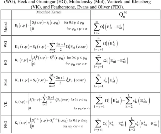
Stokes’s formula. After him, de Witte (1967); Wong and Gore (WG) (1969), Meissl (1971), Heck and Gruninger (HG) (1987), Vanicek and Kleusberg (VK) (1987), Vanicek and Sjöberg (1991), Featherstone et al. (FEO) (1998), Evans and Featherstone (2000) invented different deterministic methods for the same purpose. In Table 1, we summarise some of these methods which are developed for the SGG data and the estimators presented in Eqs. (1)- (3). In fact, this table presents the mathematical formulae of the modified kernels based on each deterministic approach and the truncation coefficient of the corresponding integral formulae.

Table 1 - Mathematical formulae of modified kernels and truncation coefficients of corresponding integral formulae according to methods of Meissl, Wong and Gore

(WG), Heck and Gruningar (HG), Molodensky (Mol), Vanicek and Kleusberg (VK), and Featherstone, Evans and Oliver (FEO).

Modified Kernel M

n

Q

M

ei

ssl

 

 

 

0 0

0 , , for 0 ,

0 for

i i

i

S r S r

K r    

          _{ }  WG

HG

 

 

 

0 0 0 , , for 0 ,

0 for

p p

i i

i

S r S r

K r    

    _{  }       M o

l

   





2

2 1

, , cos

2

M i

i i n ni

n

n

K r S r s P 

   



VK  

    0

2

0 2 1

, cos for 0

, 2

0 for L p i ki i k i k k

S r s P

K r    

     _  _{  }        



F EO

The mathematical formulae of

E

_nki , presented in Table 1, are:





2

i i i

l nl nl

l E E     



 

 





2 2 1

, , cos

2 p

i

i i l ni

n

n

K r S r P 

   





 

1 i i l nl l p E    







1

i i i l nl nl

l p E E      



 

1 i i n nl l p s E   



 

 

1 2 L

i i i i

l nl k nk

l p k

E s E



  

 





  ,   ,

 

0 0 0

, , for 0 ,

0 for

P L P L

i i

i

S r S r

K r    

    _{  }      









1 2 L

i i i i i i

l nl nl k nk nk

l p k

E E s E E



  

 

   

2

1 1

2

i i

nk i nk

k

k

E

e

u





and

2

1 1

2

i i

nk i nk

k

k

E

e

u









(6)

where

and

, i =0, 1 or 2, (7)

are the Paul coefficients of order 0, 1 and 2 and Paul (1973) proposed a recursive formula to generate zero-order one. Eshagh (2010b) presented the following recursive formulae for the first- and second-order Paul coefficients:

 









1 0

1 0

1

cos

nk nk k n n

e



n n



e



n P

P

_





P

(8)

 





 





1/2

2 1 2

0 1 1 0 1

2cos

1

2

1 1 cos

nk n n nk n k

e





P P



n n

 

e



n n







P P

.(9)

and finally we have:







 





1

0

1

1

1

1

2

2

i k

i

u

k k

i

k

k k

k

i









_





 









. (10)

 

2 2 1 2 L i i i L

n n nk k

k

E s Q



 _



(11)

2 2

2 1 2 1

2 1

L L

i i i i

n

nk k nk

k k

k k

E s Q E

k

 

 _{ }  





. (12)

4. NUMERICAL INVESTIGATIONS

In order to perform a numerical investigation into the estimation of the SGG data at the 250 km level, the EIGEN-51C geopotential model (Bruinsma et al. 2010) is used as a reference EGM for generating the gravity anomaly and gravity gradients for our simulation study. The aim is to use the gravity anomalies and the deterministically-modified integral estimators to produce the SGG data and compare their corresponding ones to those generated by the EGM. Through this study, the Tscherning-Rapp’s (1974) model is used for generating the signal spectra of the gravity anomaly. Eshagh (2009c) showed that the results of the modification of the Stokes formula in the case of using this model and EGM08 (Pavlis et al. 2008) are



 



0

cos

cos

sin

i

nk ni ki

e

P

P

d

 





 









0

cos

sin

i nk ni

e

P

d







 

more or less the same and there is no need to use EGM08 for generating the signal spectra. The truncation coefficients of the estimators are simply generated by their spectral forms. Eshagh (2010a) showed that because of the inclusion of the parameters

0

n



,



1_nand



2_n the series will be convergent due to the elevation of the satellite, but the series should be used to high degrees. He showed that a maximum degree of 5000 should be enough for this purpose. He also discussed that the recursive formulae presented by Shepperd (1982) are not suitable when the data are of satellite type. Shepperd (1982) mentioned that his formulae might be used for the altitudes below 20 km.

The cap size of integration and the degree of modification are two important factors which should be investigated for applying any integral formula and should be specified through different numerical studies. Therefore, we divide our numerical investigations into two parts, in the first part, the behaviours of the deterministically-modified kernels are presented, in the second one, the SGG data are generated using the gravity anomalies at sea level by using the modified integral estimators.

4.1 Behaviours of Isotropic Parts of the Modified Kernels

Now, the isotropic parts of the kernels of the integral estimators (1), (2) and (3) are presented. The significance of the far-zone gravity anomalies depends on these parts of the kernels. Plotting these isotropic functions shows that whether the modification has been done successfully or not. Also, it can somehow give an idea about the significance of the data being integrated and the cap size of integration. Eshagh (2014) mentioned that the contribution of the far-zone data was also dependent on the type of the data being integrated.

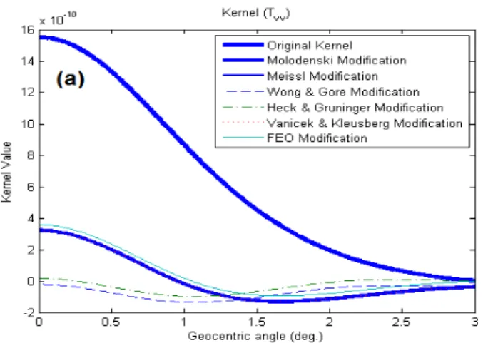
Figures 1a, 1b and 1c present the behaviours of the isotropic parts of the kernels

of the VV, VH and HH estimators. A cap size (



₀ ) of 3oand a degree of

series. Therefore,



₀plays a less significant role, but the opposite is true for the

degree modification.

The modified kernels by the VK and Mol modifications are almost coincidedandshow that the terrestrial data have the same contribution in their corresponding estimators. Featherstone (2003) presented that the fluctuation of the spheroidal Stokes kernel is because of the oscillations of the low-degree Legendre polynomials, and this fluctuation grows with the degree of spheroidal modification. Large oscillations of the kernels cause difficulties in their numerical implementations of the integral part of the estimators. Since the value of the non-modified kernels at the rim of integration cap that is close to zero, therefore, the modified kernel by the Meissl method almost coincidesthe original kernel.

The values of the non-modified kernels of the HH and VH estimators are not small at the rim of



₀therefore the modified kernels by the Meissl method deviate from the

non-modified ones. In fact, the Meissl modification needs to determine



₀by

minimising the mean squared errorof the estimator in a least-square sense.Because of the limited coverage of the terrestrial data this is not always useful. To achieve the

minimum mean squared error, we take its derivative respect to

S r

 

,



₀ and equate the

result to zero (SJÖBERG and HUNEGNAW 2000). For minimising the contribution of the far-zone terrestrial data in the modified estimators, the kernel values should be close to zero outside the integration domain. As can be seen, Figure 1 shows this issue for the modified kernels, by comparing them to the original ones, especially for the modified kernels of the VH and HH estimators. This can somehow show that the modification processes have been successful.The system of equations from which the modification parameters are obtained is ill-conditioned for the VH and HH estimators (ESHAGH,

2010a). This is due to inclusion of

u

_ki in the mathematical expressions of the elements

of the coefficient matrix of the systems.

u

_ki increases unboundedly and for large degree

of modifications, the system will be even more unstable. However, this instability is harmless and modification of the estimators will be successful if a simple regularisation method is used for solving the system Eshagh (2010a).

4.2 Generation of Satellite Gravity Gradiometry Data Using Modified Integral Estimators Over Fennoscandia

A grid of the terrestrial gravity anomalies is produced using the EIGEN-51C model to degree and order 360 with a resolution of

5

 



5

at sea level in Fennoscandia, limited between the latitudes 50° _{N and 75}° _{N and the longitudes 0° E}

and 35° _{E. The SGG data in the LNOF are generated using the same model and the}

modified integral estimators. It should be stated that, the use of EIGEN-51C to degree and order 360 is reasonable and any other EGM can be used in this respect. However, we cannot expect to recover the all frequencies to degree and order 360 due to the satellite elevation. The GOCE EGMs have been computed to degree and order 250. We have generated the gravity anomalies with a resolution of

5

 



5

to reduce the discretisation error in the integration process but we know that recovering higher frequencies than 250 is not meaningful. Table 2 shows the statistics of the mentioned gravity anomalies and the SGG data at 250 km level and Figure 3 shows their maps over Fennoscandia.

Table 2 - Statistics of gravity anomalies and SGG data in Fennoscandia

Max Mean Min Std

zz

T

(1 E) 0.430 -0.002 -0.455 0.187

xz

T

(1 E) 0.391 0.000 -0.260 0.036

yz

T (1 E) 0.210 -0.136 -0.479 0.026

xx

T

(1 E) 0.187 -0.011 -0.267 0.027

yy

T (1 E) _{0.282 -0.028 -0.319 0.028}

xy

T (1 E) 0.167 0.030 -0.122 0.017

g



(1 mGal) 73.82 3.77 -54.69 3.88

Figure 3 - a) Gravity anomaly [mGal], b)

T

_xz[E], c)T_yz [E], d)

T

_xx [E], e)T_yy, f) T_xy

The differences between the SGG data derived from the EIGEN-51C and those from the gravity anomalies are regarded as the external errors of the estimators. In the following, different



₀ and L, are considered and tested to find the best conditions

4.3 Test of Cap Size of Integration and Degree of Modification

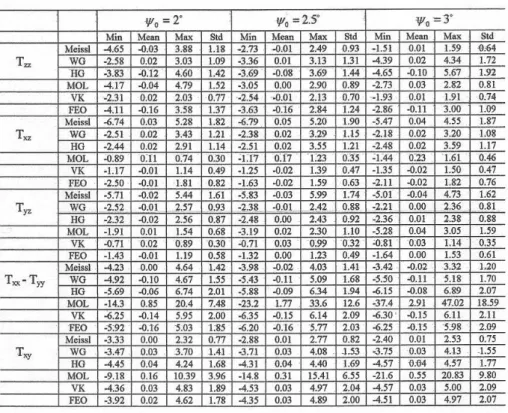
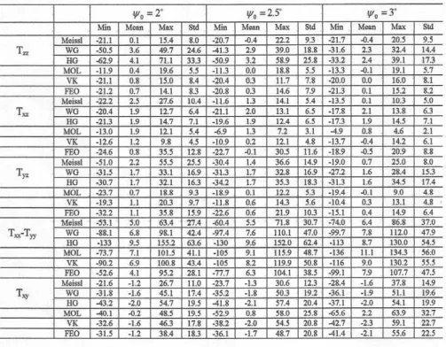
Table 3 (see appendix) presents the statistics of the differences between the generated SGG data using the integral estimators modified to degree L = 150 and

different



₀. Generally, it shows that the modified estimators can reproduce the SGG

data with an error of about 1-2 mE. This level of error reduces insignificantly by

increasing



₀ meaning that



_{0= 2}ois sufficient for integrating the gravity anomalies.

The large value of L = 150 causes that the estimators become insensitive to the choice

of



₀. The generation of

T

_xx



T

_yyis successful with an error of less than 2 mE by

some estimators and again the anomalies seem to have no impact on the quality of the

estimated

T

_xx



T

_yy and

T

_xy .

This means that the series terms of their estimators are stronger than the integral ones and have more contribution to the estimates. The estimators, modified by the Meissl, HG and WG methods have this property. The errors of the estimates, derived

by the modified estimators by MOL, increase withincreasing



₀. The reason is the

dependence of these components to the second terms of their corresponding estimators

so that by increasing



₀ insignificant changes are seen in the results.

Here, we test different L to see if the choice of a smaller L is successful according to the selected



₀. Having small L decreases the dependence of the estimators to the EGM and increases the contribution of the gravity anomalies in the integration domain. Table 4 (see appendix) presents the statistics of the differences between the generated SGG data when L = 75.

It presents that the produced SGG data are more sensitive to



₀ than the case

where L = 150, as expected. By selecting L = 75, the estimator will consider higher

weight for the gravity anomalies than the EGM. Also, when



₀ = 3o then

T

_zzis

generated with an error of less than 6 mE and

T

_xz with an acceptable accuracy level,

yz

T

with 5 mE error, but the rest of the SGG data with a lower accuracy level. One cannot find a method, which delivers the best results for all SGG data. As the table

shows, the Molodensky modified estimators deliver almost the best estimates for

T

_zz,

xz

T

and

T

_yz .

Also, the contribution of the integral term of the estimators of

T

_xx



T

_yy and

xy

Meissl methods have this property. In the case of using the MOL method the error increases with increasing



₀ due to the dependency of the estimators to the EGM.

0



= 3oseems to be suitable for this purpose. Consequently, we keep this fixed and reduce L to find the best agreement between



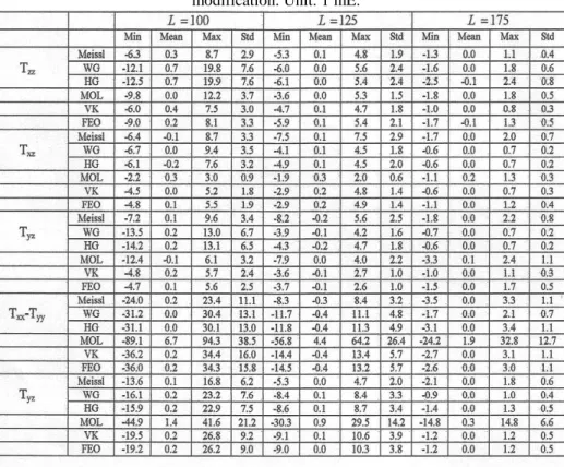
₀ = 3oand L. Table 5 shows the results of this investigation.

Table 5 (see appendix) shows the statistics of the errors of the produced SGG data

using the estimators modified with



₀ = 3o at different L . As the table presents, by

increasing L from 75 to 100, the errors of

T

_zz,

T

_xz and

T

_yz reaches to 3 mE and

T

_xyto

7 mE. By considering L= 125 even smaller errors are seen in the SGG data, which means that considering larger L is not necessary. However, for generating some of the SGG data L = 150 is required. For reproducing the HH components L = 125 and



₀ =

3oshould be enough to reach to 2-3 mE error. As the table shows, the increase of L to

175 leads to errors less than 1 mE. In short, for producing the SGG data,



₀ = 3oand

L = 150 are suitable, but



₀ = 3oand L = 125 can be suitable for some of the SGG

data. In this table, the methods of WG and HG and Meissl exhibit best results when the contribution of the second terms increase with increasing L to 175.

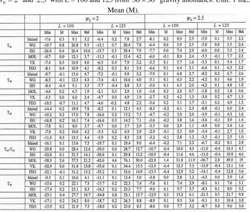
Now, we can test



₀ versus L> 75. The results are presented in Table 6 (see

appendix).



₀ is decreased to 2o and 2.5o and L = 100 and L = 125 are considered.

From the table, one can reach to accuracies of about 1-2 mE for

T

_xz and

T

_yz; and 2 mE

for

T

_zz. Therefore, their modified integral estimators with



₀ = 2.5o and L = 100 work properly. Also, when L = 125 the SGG data an error of 2-3 mE can be produced

with



₀ = 2o and



₀ = 2.5ofor the VV and VH gradients. This means that L = 125

is suitable and the estimator is sensitive enough to



₀ and subsequently to the gravity

anomalies.

5. CONCLUDING REMARKS

The cap size of integration (



₀) and the degree of modification (L), which are

two important parameters to be selected before using the estimators, should beL=125

and



₀= 2.5o, the VV gradient can begenerated with an error less than 2 mE over

for the VH gradients and L=125 and



₀=3ofor the HH gradients. Insignificant

variations are seen in the quality of the generated gradients due to changes in the resolution of the terrestrial gravity anomalies. Our numerical studies show that, in most cases, the Molodenski modification delivers better results than the rest of the deterministic modification methods.

REFERENCES

ABDALLA, A. and TENZER, R. The global geopotential and regional gravimetric geoid/quasigeoid models testing using the newly adjusted levelling dataset for New Zealand. Applied Geomatics. 2012.

ABDALLA A., FASHIR H. H., ALI A. and FAIHEAD D. Validation of recent GOCE/GRACE geopotential models over Khartoum state-Sudan, Journal of Geodesy and Sciences. 2(2): 88-97. 2012.

ALBERTELLA A., MIGLIACCIO F., and SANSÒ F. GOCE: The Earth Field by Space Gradiometry. Celestial Mechanics and Dynamic Astronomy, 83, 1-15. 2002.

BALMINO G., PEROSANZ F., RUMMEL R., SNEEUW N., SÜNKEL H. AND WOODWORTH P., European Views on Dedicated Gravity Field Missions: GRACE and GOCE. An Earth Sciences Division Consultation Document, ESA, ESD-MAG-REP-CON-001. 1998.

BALMINO G., PEROSANZ F., RUMMEL R., SNEEUW N. and SÜNKEL H. CHAMP, GRACE and GOCE: Mission Concepts and Simulations. Bollettino di Geofisica Teorica ed Applicata, 40, 3-4, 309-320. 2001.

BOUMAN, J., KOOP, R. Error assessment of GOCE SGG data using along track interpolation. Advanced Geoscience. 1, 27–32. 2003.

BOUMAN, J., KOOP, R., HAAGMANS, R., MULLER, J., SNEEUW, N. TSCHERNING, C.C., VISSER, P. Calibration and validation of GOCE gravity gradients, Paper presented at IUGG meeting, pp. 1–6. 2003.

BOUMAN, J., KOOP, R., TSCHERNING, C.C., VISSER, P. Calibration of GOCE SGG data using high-low STT, terrestrial gravity data and global gravity field models. Journal of. Geodesy. 78, 124–137. 2004.

BRUINSMA S.L., MARTY J.C., BALMINO G., BIANCALE R., FOERSTE C., ABRIKOSOV O. (1) and NEUMAYER H.(1). GOCE Gravity Field Recovery by Means of the Direct Numerical Method, presented at the ESA Living Planet Symposium 2010, Bergen, June 27 - July 2 2010, Bergen, Norway.

ESA Gravity Field and Steady-State Ocean Circulation Mission, ESA SP-1233(1), Report for mission selection of the four candidate earth explorer missions. ESA Publications Division, pp. 217, July, 1999.

ESHAGH M. On satellite gravity gradiometry, Doctoral dissertation in Geodesy, Royal Institute of Technology (KTH), Stockholm, Sweden. 2009a

ESHAGH M. Alternative expressions for gravity gradients in local-north oriented frame and tensor spherical harmonics, Acta Geophysica, 58, 215-243. 2009b. ESHAGH M. Least-squares modification of stokes' formula with EGM08, Journal of

Geodesy and Cartography, 35(4): 111–117. 2009c.

ESHAGH M. Least-squares modification of extended Stokes’ formula and its second -order radial derivative for validation of satellite gravity gradiometry data, Journal of Geodynamics, 49, 92-104. 2010a.

ESHAGH M. Towards validation of satellite gradiometric data using modified

version of 2nd order partial derivatives of extended Stokes’ formula, Artificial Satellites, 44, 4, 103-129. 2010b.

ESHAGH M. On the reliability and error calibration of some recent Earth's gravity models of GOCE with respect to EGM08, Acta of Geodesy and. Geophysic. Hung., 48(2): 199-208. 2013.

ESHAGH M. From tensor to vector of gravitation, Artificial Satellites, (accepted). 2014.

ESHAGH M. and ABDOLLAHZADEH M. Semi-vectorization: an efficient technique for synthesis and analysis of gravity gradiometry data. Earth Science Informatics,. 3, 149-158. 2010.

ESHAGH M. and ABDOLLAHZADEH M., Software for generating gravity gradients using a geopotential model based on irregular semi-vectorization algorithm. Computer and Geoscience., 32, 152-160. 2011.

ESHAGH M. and EBADI S. Geoid modelling based on EGM08 and the recent Earth gravity models of GOCE, Earth Sciece. Inf. 6:113-125. 2013.

ESHAGH and EBADI. A strategy to calibrate errors of earth gravity models, Journal of Applied Geophysics. 103, 215–220. 2014.

ESHAGH M. and ROMESHKANI M. Generation of vertical-horizontal and horizontal-horizontal gravity gradients using stochastically modified integral estimators. Advances in Space Research, 48, 1341−1358. 2011.

EVANS JD, FEATHERSTONE WE Improved convergence rates for the truncation error in geoid determination. Journal of Geodesy, 74: 239-248. 2000.

FEATHERSTONE W.E., EVANS J.D. and OLLIVER J.G. A Meissl modified Vanicek and Kleusberg kernel to reduce the truncation error in gravimetric geoid computations. Journal of Geodesy, 72, 3, 154–160. 1998.

FEATHERSTONE W.E. Software for computing five existing types of deterministically modified integration kernel for gravimetric geoid determination, Computers & Geosciences, 29, 183-193. 2003.

I., SCHUH W.-D., JÄGGI A., PRANGE L., HAUSLEITNER W., BAUR O., KUSCHE J. The combined satellite-only global gravity field model GOCO02S, presented at the 2011 General Assembly of the European Geosciences Union, Vienna, Austria, April 4-8, 2011. 2011.

GUIMARAES G.N., MATOS A. C. O. C. and BILTZKOW D. An evaluation of recent GOCE geopotential models in Brazil, Boletim de Ciências Geodésicas. 2(2): 144-155. 2012.

HAAGMANS R. PRIJATNA K. and OMANG O. An alternative concept for validation of GOCE gradiometry results based on regional gravity, In Proc. Gravity and Geoid 2002, GG2002, August 26-30, Thessaloniki, Greece. 2002.

HECK B. and GRUNINGER W. Modification of Stokes’s integral formula by

combining two classical approaches. Proceedings of the XIX General Assembly of the International Union of Geodesya nd Geophysics, 2. Vancouver, Canada, pp. 309–337. 1987.

HIRT C., GRUBER T. and FEATHERSTONE W.E. Evaluation of the first GOCE static gravity field models using terrestrial gravity, vertical deflections and EGM2008 quasigeoid heights, Journal of Geoidesy. 85: 723-740. 2011. JANAK J and PITONAK M. Comparison and testing of GOCE global gravity models

in central Europe, Journal of Geodesy and Science. 1(4): 333-347. 2011. JARECKI F., KAREN K.I., WOLF, H. DENKER and J. MULLER. Quality

Assessment of GOCE Gradients, Observation of the Earth System from Space 2006, pp 271-285. 2006.

KERN M. and HAAGMANS R. Determination of gravity gradients from terrestrial gravity data for calibration and validation of gradiometric GOCE data, In Proc. Gravity, Geoid and Space missions, GGSM 2004, IAG International symposium, Portugal, August 30- September 3, pp. 95-100. 2004

KERN M., PREIMESBERGER T., ALLESCH M., PAIL. R., BOUMAN J. and KOOP R. Outlier detection algorithms and their performance in GOCE gravity field processing, Journal of Geodesy, 78, 509-519. 2005.

MEISSL P. Preparations for the numerical evaluation of second-order Molodenskii-type formulas. Report 163, Department of Geodetic Science and Surveying, The Ohio State University, Columbus, OH, 72pp. 1971.

MOLODENSKY M.S., EREMEEV V.F. and YURKINA M.I. Methods for study of the external gravity field and figure of the Earth. Translated from Russian (1960), Israel program for scientific translation, Jerusalem. 1962.

MOLODENSKY, M.S., Grundbegriffe der Geodatischen Gravimetrie. VEB Verlag Technik, Berlin. 1958.

MÜLLER J., DENKER H., JARECKI F. and WOLF K.I. Computation of calibration gradients and methods for in-orbit validation of gradiometric GOCE data. In: Lacoste H. (Ed.), Proceedings of the Second International GOCE User

Workshop “GOCE, The Geoid and Oceanography”, 8-10 March 2004,

PAIL, R. Local gravity field continuation for the purpose of in-orbit calibration of GOCE SGG observations. Advanced Geoscience. 1, 11–18. 2003.

PAIL R., GOIGINGER H., SCHUH W.D., HOECK E., BROCKMANN J.M., FECHER T., GRUBER T., MAYER GUERR T., KUSCHE J., JAEGGI A. and RIESER D. Combined satellite gravity field model GOCO01S derived from GOCE and GRACE, Geophics Resolution Letter., 37, L20314. 2010.

PAIL R., BRUINSMA S., MIGLIACCIO F., FOERSTE C. GOIGINGER H., SCHUH W. D., HOECK E., REGUZZONI M., BROCKMANN J. M., ABRIKOSOV O., VEICHERT M., FECHER T., MAYRHOFER R., KRASBUTTER I., SANSO F. and TSCHERNING C.C. First GOCE gravity field models derived by three different approaches, Journal of Geodesy. 85: 819-843. 2011.

PAUL M.K. A method of evaluating the truncation error coefficients for geoidal height, Bulletin Geodesique, 110, 413-425. 1973.

PAVLIS N., HOLMES SA., KENYON S. C. and FACTOR JK. An Earth Gravitational model to degree 2160: EGM08. Presented at the 2008 General Assembly of the European Geosciences Union, Vienna, Austria, April 13-18, 2008.

ROMESHKANI M., Validation of GOCE Gravity Gradiometry Data Using Terrestrial Gravity Data. M.Sc. Thesis, K.N.Toosi University of Technology, Tehran, Iran. 2011.

RUMMEL R., BALMINO G., JOHANNESSEN J., VISSER P. and WOODWORTH P. Dedicated gravity field missions-principles and aims, Journal of Geodynamics, 33:3-20. 2002.

SHEPPERD S. W.) A recursive algorithm for evaluating Molodeski-type truncation error coefficients at altitude, Bulletin Geodesic. 56: 95-105. 1982.

Sjöberg L.E. Least-squares combination of satellite harmonics and integral formulas in physical geodesy, Gerlands Beitr. Geophysik, Leipzig 89(5):371-377. 1980. SJÖBERG L.E. Least-squares combination of terrestrial and satellite data in physical

geodesy, Annals of Geophysics., t. 37: 25-30. 1981.

SJÖBERG L.E. and HUNEGNAW A. Some modifications of Stokes' formula that account for truncation and potential coefficient errors. Journal of Geodesy, 74, 232-238. 2000.

SPRLAK M, NOVAK P Integral transformations of gradiometric data onto a GRACE type of observable. Journal of Geodesy 88:377–390. 2014a

SPRLAK AND NOVAK. Integral transformations of deflections of the vertical onto satellite-to-satellite tracking and gradiometric data. Journal of Geodesy 88: 643-657. 2014b.

SPRLAK M. GERLACH C. and PETTERSEN B. R. Validation of GOCE global gravity field models using terrestrial gravity data in Norway, Journal of Geodesy and Geosciences. 2(2):134-143. 2012.

TAPLEY B., RIES J. BETTADPUR S., CHAMBERS D., CHENG M., CONDI F., GUNTER B., KANG Z., NAGEL P., PASTOR R., PEKKER T., POOLE S. and WANG F. GGM02-An improved Earth gravity field model from GRACE. Journal of Geodesy., 79:467-478. 2005.

TOTH GY., ADAMJ., FOLDVARY L., TZIAVOSI.N., DENKER H. Calibration/validation of GOCE data by terrestrial torsion balance observations, A Window on the Future of Geodesy International Association of Geodesy Symposia Volume 128, 2005, pp 214-219. 2005

TSCHERNING C.C. and RAPP R. Closed covariance expressions for gravity anomalies, geoid undulations and deflections of vertical implied by anomaly degree variance models. Rep. 355. Dept. Geod. Sci. Ohio State University, Columbus, USA. 1974.

TSCHERNING C. C., VEICHERTS M. and ARABELOS D. Calibration of GOCE gravity gradient data using smooth ground gravity, In Proc. GOCINA workshop, Cahiers de center European de Geodynamique et de seismilogie, Vol. 25, pp. 63-67, Luxenburg. 2006.

VANICEK P. and KLEUSBERG A. The Canadian geoid Stokesian approach. Manuscripta Geodaetica 12, 2, 86–98. 1987.

VANICEK P. and SJÖBERG L.E. Reformulation of Stokes’s theory for higher than

second-degree reference field and modification of integration kernels. Journal of Geophysical Research—Solid Earth 96 (B4), 6529–6539. 1991.

WANGER C.A. and MCADOO D. C. Error calibration of geopotential harmonics of recent and past gravitational fields, Journal of Geodesy. 86: 99-108. 2012. WENZEL H.G. (1981) Zur Geoidbestimmung durch kombination von

schwereanomalien und einem kugelfuncationsmodell mit hilfe von integralformeln. Zeitschrift fur Geodasie, Geoinformation und Landmanagement, 106, 3, 102-111. 1981.

WONG, L. and GORE, R. Accuracy of geoid heights from modified Stokes kernels. Geophysical Journal of the Royal Astronomical Society18, 81–91, 1969. WOLF K. I.. Kombination globaler Potentialmodelle mit terrestrischen

Schweredaten für die Berechnung der zweiten Ableitungen des Gravitationspotentials in Satellitenbahnhöhe. Wissenschaftliche Arbeiten der Fachrichtung Geodäsie und Geoinformatik der Universität Hannover 264, University of Hannover, Hannover, Germany. 2007.

ZIELINSKI, J.B., PETROVSKAYA, M.S. The possibility of the calibration/ validation of the GOCE data with the balloon-borne gradiometer. Advanced Geosciences. 1, 149–153.. 2003.

APPENDIX

Table 3 - Statistics of errors of generated SGG data at different



₀ using modified

Table 6 - Statistics of errors of generated gradients using the modified estimator with

0 2

  o

and 2.5o