http://dx.doi.org/10.1590/S1982-21702015000400049
Article
FAST INTEGER AMBIGUITY RESOLUTION IN GPS KINEMATIC
POSITIONING USING LEFT NULL SPACE AND MULTI-TIME (INVERSE)
PAIRED CHOLESKY DECORRELATION
Solução rápida da ambiguidade GPS no posicionamento cinemático usando espaço
nulo à esquerda e descorrelação de Cholesky multi-temporal (inversa) pareada
Rong Duan Xiubin Zhao Chunlei Pang Ang Gong
College of Information and Navigation, Air Force Engineering University, Xi’an, China [email protected]
Abstract:
o
Keywords: GPS; Integer ambiguity; SVD; Multi-time (inverse) paired Cholesky decomposition
Resumo:
Com o objetivo de solucionar os problemas envolvendo enorme quantidade de cálculos na resolução de ambiguidade com multiplas épocas e inversão de matriz de alta ordem como ocorre no posicionamento relativo cinemático GPS, um algoritmo modificado para resolução rápida da ambiguidade é proposto. Em primeiro lugar, Decomposição de Valor Singluar (SVD) é aplicada para construir a matriz de espaço nulo de modo a eliminar os parâmetros das componentes da linha de base, o qual é capaz de separar os parâmetros de ambiguidade dos parâmetros de posição de forma eficiente. O Filtro de Kalman é aplicado somente para estimar os parâmetros de ambiguidade de tal forma que a solução float em tempo real é obtida. Então, é adotada a decomposição de Cholesky ordenada e multi-temporal (inversa) pareado (multi-time paired Cholesky decorrelation) para a descorrelação das ambiguidades. Após o pré-processamento dos elementos diagonais e da ordenação destes elementos de acordo com os resultados da decomposição de Cholesky, a eficiência da decomposição e decorrelação é melhorada. Posteriormente, o algoritmo de busca inteiro implementado no método LAMBDA, é usado para estimar a ambiguidade inteira. Para verificar a validade e eficácia do algoritmo proposto, experimentos no modo estático e cinemático foram realizados. Os resultados experimentais mostram que este algoritmo tem o bom desempenho de descorrelação e precisão da solução float, com aumento eficaz na velocidade de cálculo. A acurácia do posicionamento em linha de base estática apresentou menor que 1 cm e no caso cinemático foi inferior a 2 cm, o que indica que o método pode ser usado para o posicionamento cinemático rápido com alta precisão da fase.
Palavras-chave: GPS; Ambiguidade; decomposição de SVD; decomposição de múltipla (reverso) dupla Cholesky
1. Introduction
To solve this problem, a new algorithm is proposed to implement fast integer ambiguity resolution of kinematic application. Firstly, SVD decomposition and transformation are applied to construct a left null space matrix to remove baseline coordinate parameters and separate ambiguity parameters from position parameters. Kalman filter is used to estimate only the ambiguity parameters that can be used to acquire real-time float solution of integer ambiguity. Then, diagonal entries of covariance matrix are sorted, and multi-time (inverse) paired Cholesky decomposition is applied for the decorrelation of ambiguity. After diagonal elements preprocessing and diagonal elements sorting according to the results of Cholesky decomposition, the efficiency of decomposition and decorrelation is improved. Finally, integer ambiguity is estimated by the integer search algorithm of LAMBDA method. Static and kinematic experiments prove the correctness and feasibility of the new algorithm.
2. Fast Calculation of Ambiguity Float Solution Based on SVD
Decomposition
Suppose that base station and mobile station observe n satellites synchronously, and each epoch can construct n-1 double difference carrier phase measurement equations. For the ith epoch, GPS double difference carrier phase linear observation equations are generally expressed as follows
where n1
i
L R denotes the observation vector of double difference (DD) carrier phase at the ithepoch,
which is the difference between observed value and the calculated one. (n1) 3
i
A R is coefficient matrix at the ithepoch. Xi is the unknown parameter vector of 3D baseline.
1
n
N Z is the unknown DD ambiguity parameters vector with n-1 dimensions, which is independent of the epoch.
1 1 1
( L, L, L)
diag
L
B is the coefficient matrix with n-1 dimensions, where L1 is the L1 carrier
wavelength. εiis the measurement noise vector.
In fast positioning, it is preferable that fewer epochs or even single epoch can implement positioning. According to Equations 1, it has 3 rank deficiencies when calculating in single epoch, thus the LS method is unavailable. What is adopted in common is to increase the number of observation epochs, i.e., to increase equations. For m epochs, corresponding equations are
o
High-order matrix inversion is a problem (Liu et al., 2005; Liu et al., 2013) of huge computation in directly solving Equations 3. In order to obtain high precision ambiguity float solution, at least 200 to 400 epochs is needed, which results in very high-order matrix with about 600 to 1200 dimensions. Thus, it can not meet the requirement of real-time kinematic positioning. In fact, only the ambiguity float solution and its covariance are concerned. Therefore this paper applies SVD decomposition to coefficient matrix (Timothy, 2010). Baseline component correction vector is eliminated by constructing left null space matrix LAaccording to U matrix features. In this way, ambiguity
parameters can be successfully separated from position parameters, with reduced matrix dimension. Based on SVD decomposition, transformation steps are as follows
(1) Solve the left null space matrix of coefficient matrix Ai. SVD decomposition is carried out to Ai,
and T
i
0
A U V
0 0
, where U is (n 1) (n 1) unitary matrix, V is 3 3 unitary matrix,
1 2 ( , , , r) diag
L
,rrank(Ai) and i denotes all non-zero singular values of matrix Ai.
(2) Divide the matrix Uas 1 2
(n 1)r (n 1) (n1 r)
U U M U . What can be easily proved is the following formula:
2 i
T A
L U , namely 0
i
A i
L A
Proof: the formula above is rewritten as
11 2 1 1
2 T T i T
M 0 V
A U U U V
0 0 V
, then multiplied by 2
T
U on
both sides, therefore
2 ( 2 1) 1
T T T
i
U A U U V 0
2 1
H
U U 0 .
(3) Multiply Equations (3) by left null space matrixLAion both sides; and the transformed equation is
Where
k
k A k
Z L L ,
k
k A
H L B. Vk is the measurement white noise with mean zero and variance
cov( , )
k k k
R V V EV Vk kT 2L LA TA2I.
Since the state vector of integer ambiguity N is constant, time update process (prediction process) during Kalman filtering can be simplified as follows
Kalman filter Measurement update process (calibration process) is given as
Among Equations 8, Kk is filtering gain; I is unit matrix. According to the initial value of state
vectorNˆ0and the estimation error covarianceQNˆ0, the optimal estimation of ambiguity state vector and estimation error covariance at any time can be obtained. As indicated from the Filtering equations above, state parameters, such as position parameters and velocity parameters, are eliminated during the process of calculation. Therefore, the computation load is greatly reduced by avoiding of high-order matrix inversion, which contributes to ambiguity estimation in real-time kinematic applications.
3. Sorting and Multi-Time (Inverse) Paired Cholesky Decomposition
for Decorrelation
Real-time float solution of ambiguity can be obtained based on SVD decomposition and Kalman filtering. Nevertheless, during a short period of observing time in actual kinematic positioning environment, double difference observation may lead to inferior geometric structure between the ground station and satellites, which in turn leads to strong correlation between DD measurements. This strong correlation extends multi-dimensional ellipsoid search space and integer ambiguity search results are far from expectation. To solve this problem, the covariance matrix of float solution needs to be decomposed and diagonalized as much as possible. In this way, the correlation between ambiguities of DD phase measurements can be reduced, which makes the search ellipsoid space closer to sphere, minimizing length of search interval and improving the efficiency in the search of integer ambiguity fixed solution.
o
realize continuous decorrelating (Xu, 2001;Zhou, 2011; Zhou and He, 2014). Before Cholesky decomposition, sorting the diagonal elements in ambiguity covariance matrix (ascending or descending) can reduce condition number of matrix and effectively improve the performance of matrix decomposition (Liu et al., 1999; Chen and Wang, 2002; Huang and Chen, 2010). Compared to this traditional method, this paper applies a method of diagonal elements preprocessing after Cholesky decomposition. New algorithm orders diagonal elements of the matrix according to values after decomposition, in contrast to existing method according to values before decomposition. Consequently, our new method is closer to the goal of arranging the larger diagonal element to the smaller row before decomposition for UDUT, and LDLT decomposition is on the contrary.
The sorting depends on the relative size of the diagonal candidate values
v ip, p n
which are computed by pre-compute formula, instead of relative size of the diagonal elements of the original covariance matrix. Adjusting matrix could only be determined after pre-computing the candidate elements vp of diagonal elements di, which ensures that the adjusted covariance matrix after Cholesky decomposition acquire the best decorrelation performance.After sorting based on the result of Cholesky decomposition, bigger diagonal entries of UDUT result is adjusted to a smaller I positions in diagonal line, and LDLT vice versa. The value of each diagonal element after adjustment is much closer to one another, and the validity of matrix decomposition is improved, so is the decorrelation. Then, the efficiency and quality of ambiguity discrete search is improved. The steps of sorting and multiple (inverse) paired Cholesky decomposition are as follows
I) Modified integer UDUT decomposition
1) LetJ0QNˆ qij n n ,i1, 2,L ,n. Perform the following steps to J0 row by row:
a) Pre-compute candidate elements
In Equations 9, cpjdenotes the candidate entry in unit upper triangular matrix U and vpdenotes the
candidate in diagonal matrix D.
b) Select the element vi to meet i max
p i p nv v
, and its index numberMip. LetuijcMj(i j),
i
i M
d v ,uij,didenotes the elements in modified Cholesky decomposition U and Drespectively.
c) Adjust variance-covariance matrix according to the index number constructed from the last step: ( , ) 1 ( , )
T i i i Mi i i i Mi
J S J S . WhereSi( ,i Mi)is adjusting matrix, obtained by exchange of ithrow and M thi row in unit matrixIn n . In particular, Si( ,i Mi)In n wheniMi.
2) Modified UDUT decomposition is obtained by the previous step, where U [uij n n] ,
1 2 ( , , , n) diag d d d
L
D , then one can get that T
n
1 1 1 1 ˆ ( , ) ( 1, ) (1, )
n n Mn n n Mn M
L
S S S S .
3) Let entries in upper triangular be integers and calculate the transformation matrix
U 11by matrix inversion, then the covariance matrix after modified UDUT transformation isII) Modified integer LDLT decomposition
1) Let 0 uˆ ij
n n
q
J Q ,i1, 2,L ,n, Perform the following steps to J0 row by row.
a) Pre-compute candidate elements
In Equations 11, fpjis the candidate element in unit lower triangular matrix L and vpdenotes the
candidate element in diagonal matrix D.
b) Select element vi to meet i min
p i p nv v
, and its index numberMip. Letlij fMj(i j),
i
i M
d v , and lij ,di denotes the elements in modified Cholesky decomposition L and D
respectively.
c) Adjust variance-covariance matrix according to the index number from the last step:
1
( , ) ( , )T i i i Mi i i i Mi
J G J G , where Gi( ,i Mi)is adjusting matrix, obtained by exchange of ithrow
and M thi row in unit matrixIn n . In particular, Gi( ,i Mi)In n wheniMi.
2) Modified LDLT decomposition is obtained by the previous step, which is L[ ]lij n n ,
1 2 ( , , , n) diag d d d
L
D , then one can get that n
T
J LDL , Jn GQ Gˆ uˆˆT , where
1 1 1 1
ˆ ( , ) ( 1, ) (1, )
n n Mn n n Mn M
L
G G G G 。
3) Let entries in lower triangular be integers, calculate the transformation matrix
L11by matrix inversion, then the covariance matrix after modified LDLT transformation isIII) Check whether 1 1
o
indicates that the correlation between the undetermined ambiguity is quite strong, and the process is back to step I) and go on until
L11becomes unit matrix, where the decomposition stops (Details of the proof of the correctness of this decorrelation method are discussed in Appendix).Conduct the modified integer UDUT decomposition and LDLT decomposition repeatedly. Assuming that iteration is executed for m times, and
L11is transformed to be a unit matrix, the final transformation matrix is going to beCorrespondingly, the covariance matrix of ambiguity after the transformation is
Integer ambiguity float solution is
Finally, integer ambiguity is estimated by the integer search algorithm of LAMBDA method. z is searched using Equations 16 to minimize the object function as the estimatedzˆ
Then perform inverse transformation
The original space of ambiguity is therefore obtained.
4. Experimental Analysis
4.1 Static Positioning and Result Analysis
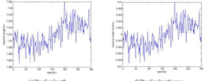
In order to validate the correctness and feasibility, static test was carried out. The data was acquired at ten thirty-one on May 16, 2013, on the top Air Force Engineering University Taoyuan campus laboratory building. Two NovAtel receivers were deployed with type OEM628 as one base station and another mobile station. All stations are installed GPS-702-GG GPS dual-frequency antenna. The recording sampling rate is 1 s. In this case, the baseline length is 7.812 m. GPS data were collected in half an hour tracking 7 satellites with 10° elevation mask: PRN6, PRN8, PRN11, PRN15, PRN17, PRN24, and PRN28. In order to reduce the errors' effect, PRN24 with maximal elevation was chosen as the reference satellite. Actual data was processed by proposed algorithm in simulation. After 120 epochs, integer ambiguity was estimated. Then, integer ambiguity was substituted back to the algorithm to compute the fixed solution, which is used to make a comparison with the real value.
Figure 1: Baseline Length and its error.
Figure 1 shows the length of baseline and its error. As can be seen from the figure baseline length error of proposed new algorithm is less than 1 cm, which indicates some good performance of accuracy.
4.2 Kinematic Positioning and result analysis
o
4.2.1 Verification scheme
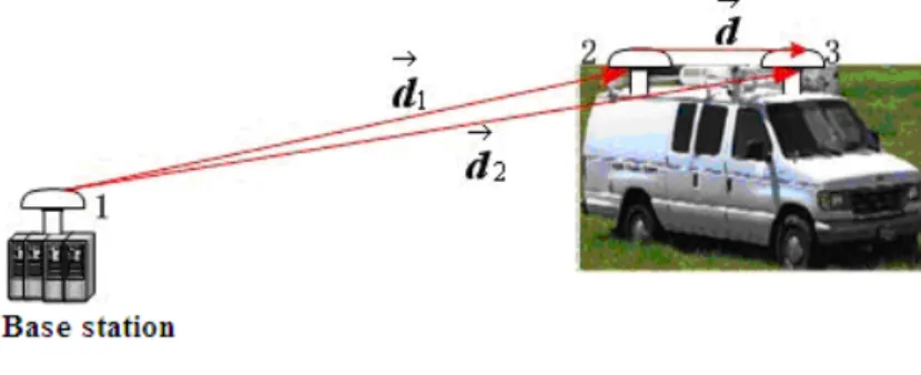
Test conditions being the same with that of static test, dual mobile station are applied, due to the fact that dynamic changes of baseline with a much longer distance and accuracy of the algorithm can not be validated directly, as shown in Figure 2. Base station is placed in open area under the Lab building and two mobile stations are placed on the top of the vehicle. One is at the head and another one is at the rear, 2.115 m apart. After a short static period, the vehicle began to go around in circles, 200 meters away from the building. Original measurements data and epoch data (L1 frequency) were collected separately and processed by the proposed fast new algorithm one epoch to another.
Figure 2: Sketch of algorithm validation embodiment.
As is shown in Figure 2, the baseline between antenna 2 and antenna1 is computed and named as
1
d vector, so was the baseline between antenna 3 and antenna 1, named as d2vector. The baseline
between antenna 2 and antenna 3 is fixed and named as d . It is easy to know that dd2d1. so
1 2
d d d . Then it is compared with fixed length of baseline d to verify the accuracy of relative position.
4.2.2 Experiments and Results Analysis
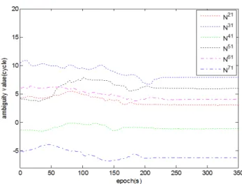
Figure 3: All the float solution of double difference ambiguities.
As can be seen from Figure 3, all the float ambiguities present a trend that approximately equal to the true value at the time of epoch 168, and the filter starts to become stabilize state. At the same time, different epochs of data are resolved by using the proposed approach and the conventional Kalman filter respectively. The results comparison of two methods in which parts of continuous epochs around epoch 168 (i.e., epoch 168 as the critical point) are selected is shown in Table 1.
Table 1: Results comparison of two methods
Table 1 shows that precision of ambiguity float solution calculated by the proposed method is better than conventional method. In addition, the average calculation time of both methods for Table 1 are respectively counted. Average calculation time of this new method is 1067 ms, while the conventional Kalman filtering method is 1703 ms. The reason is that the conventional Kalman filter needs to simultaneously estimate all the parameters such as position parameters, velocity parameters and ambiguity parameters, while in the new algorithm, SVD decomposition transform of the coordinate coefficient matrix is applied to construct the left null space matrix in order to eliminate the baseline coordinate vector parameters, thereby the Kalman filter equations can be established to estimate only the ambiguity parameters. This will not only improve the computing speed, but also improve the accuracy of float solution, which contributes to the fast resolution of ambiguity.
o
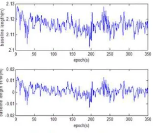
integer ambiguities are fast estimated when epoch number is 168 and 177 respectively, the Kalman filter is becoming stable gradually and the integer ambiguity can be computed rapidly. The relative position between mobile station 2 and station 3 is computed by the validation scheme described above. The length and error of baseline are shown in Figure 4(a) and the elevation and azimuth of baseline are shown in Figure 4(b).
As is shown in Figure 4, the computed position relationship between mobile station and base station is consistent with the reality. The errors of elevation and azimuth are stable in a small angle because of the circle motion of vehicle on the ground. During the test, with good signal quality, baseline error is limited within 2 cm, which indicates that ambiguity is correctly estimated. As the length of baseline, elevation and azimuth are all computed based on the relative position between mobile stations, so making the length of baseline as criterion is practical and scientific, which further verifies the correctness of the algorithm.
Figure 4: Relative position of the mobile station 2 and station 3.
Figure 5: The r and e of ambiguity covariance matrix before and after decorrelation.
As is indicated in Figure 5(a), decorrelation coefficient rbefore is near 0 before decorrelation, which indicates strong correlation between ambiguities. The spectral condition number ebefore is large in Figure 5(b), which indicates a flat search space, also reflecting the strong correlation. After decorrelation, the decorrelation coefficient rafter becomes larger and approaches 1. At the same time, its spectral condition number eafter is greatly reduced and covariance matrix is closer to diagonal one. Correlation between different ambiguities is reduced successfully, which indicates the feasibility and good performance of decorrelation of the proposed algorithm.
5. Conclusions
In this paper, the static and kinematic tests and analysis show that the proposed algorithm for ambiguity fast resolution is feasible, the static baseline error is less than 1cm and kinematic baseline error is less than 2cm. These results verify the correctness and effectiveness of the algorithm.
SVD decomposition is applied to construct the left null space of matrix to eliminate the baseline coordinate parameters which can separate the ambiguity parameters from the position parameters. Thus Kalman filter is used to estimate only the ambiguity parameters in the new algorithm, which greatly reduces the amount of computation. Computation speed are increased, which means its real-time capacity.
Sorting and multiple (inverse) Cholesky decompositions are performed for ambiguity decorrelation, adopting method of diagonal entries pre-processing and adjusting the order of diagonal entries according to values by Cholesky decompositions. The effectiveness of matrix decomposition is well ensured and much smaller conditional number is obtained, thereby performance of decorrelation is improved, which contributes to ambiguity search efficiency and correctness.
o
have a broad application prospects for airborne platform fast positioning and attitude determination and for precision approach and landing system. The proposed method also needs further improvement in some specific engineering implementation.
ACKNOWLEDGMENTS
This work is supported by China National Natural Science Foundation of China (No: 61273049). The authors also gratefully acknowledge the helpful comments and suggestions of the reviewers, which have improved the presentation.
REFERENCES
Blewitt and Geoffrey. “Carrier phase ambiguity resolution for the Global Positioning System applied to geodetic baselines up to 2000 km.” Journal of Geophysical Research Atmospheres, 94(B8), 10187-10203, 1989.
Chen, S. X., Wang, Y. S. “New algorithm for GPS ambiguity decorrelation.” Acta Aeronautica Et Astronautica Sinica”, 23(6), 542-546, 2002.
Euler, H. J., Landau, H. “Fast GPS ambiguity resolution on-the-fly for real-time application. Proceedings of sixth International geodetic symposium on satellite positioning”, Columbus, Ohio. March, 17-20, 1992.
Frei, E., Beulter, G. “Rapid static positioning based on the fast ambiguity resolution approach FARA: Theory and First Results.” Manuscripta Geodaetica 15(6), 325-356, 1990.
Hatch, R. “Instantaneous ambiguity resolution.” IAG International Symposium No. 107, Banff, Alberta, Cananda, 99-308, 1990.
Hofmann-wellenhoff, B., Lichtenegger, H., Collins, J. “Global Positioning System: Theory and Practice, fifth ed.” Springer-Verlag, Berlin, 2001.
Huang, Z. Y., CHEN, S. J. “Modified GPS ambiguity white filtering algorithm.” Journal of Southwest Jiaotong University, 45(1), 150-155, 2010.
Jazaeri, S., Amiri-simkooei, A. R., and Sharifi, M. A. “Fast integer leastsquares estimation for GNSS high-dimensional ambiguity resolution using lattice theory.” Journal of Geodesy, 86(2), 123-136, 2012.
Jazaeri, S., Amiri-simkooei, A. R., and Sharifi, M. A. “On lattice reduction algorithms for solving weighted integer least squares problems: comparative study.” GPS Solutions, 18(1), 105-114, 2014. Kim, D., Langley, R. “An optimized least-squares technique for improving ambiguity resolution and computational efficiency.” ION GPS, Salt Lake City, September, 1579-1588, 1999.
Leick, A. “GPS satellite surveying, 3rd edn.” Wiley, New York, 2004.
Liu, L. T., Su, H. T., and Zhu, Y. Z. “A new approach to GPS ambiguity decorrelation.” Journal of Geodesy, 73(6), 478-490, 1999.
Geomatics and Information Science of Wuhan University, 30(10), 885-887, 2005.
Liu. N., Xiong, Y. L., and Feng, W. “An Algorithm for Rapid Integer Ambiguity Resolution in Single Frequency GPS Kinematical Positioning.” Acta Geodaetica et Cartographica Sinica, 42(2), 211-217, 2013.
Remondi, Benjamin W. “Pseudo-kinematic GPS results using the ambiguity function method.” Journal of Navigation, 42(1), 109-165, 1991.
Teunissen, P. J. G. “A new method for fast carrier phase ambiguity estimation.” Proceedings of IEEE Position Location and Navigation Symposium PLANS’94, Las Vegas, 562-573, 1994.
Teunissen, P. J. G. “The least-squares ambiguity decorrelation adjustment: a method for fast GPS integer ambiguity estimation.” Journal of geodesy, (70), 65-82, 1995.
Teunissen, P. J. G, Verhagen S. “GNSS ambiguity resolution: when and how to fix or not to fix?.” A symposium on theoretical and computational geodesy, Springer, Berlin, 143-148, 2008.
Timothy, S. “Numerical Analysis.” Posts & Telecom Press, 2010.
Tomoji, T., Akio, Y. “Kalman-filter-based integer ambiguity resolution strategy for long-baseline RTK with ionosphere and troposphere estimation.” ION GNSS 2010. Portland, 161-171, 2010. Xu, P. L. “Random simulation and GPS decorrelation.” Journal of Geodesy, 75(7),408-423, 2001. Zhou, Y. M. “A new practical approach to GNSS high-dimensional ambiguity decorrelation.” GPS Solutions, 15(4), 325-331, 2011.
Zhou, Y. M, He, Z. “Variance reduction of GNSS ambiguity in (inverse) paired Cholesky decorrelation transformation.” GPS Solutions, 18, 509-517, 2014.
Recebido em Abril de 2015. Aceito em Setembro de 2015.
APPENDIX
o T ˆ 0 T T decomposition
1 1 0 1 1 1 1 1
2 2 1 1 0 1 1 2 2 2
decomposition
2 2
1 1 1 1 0 1 1
1 1
de
(1, ) (1, )
(2, ) (1, ) (1, ) (2, )
( , ) ( 1, ) (1, ) (1, )
( 1, ) ( , )
N
T
T T
T
n n n n
T T
n n n n n
M M
M M M M
n M n M M M
n M n M
M L L UDU J Q UDU UDU
S J S U , D
S S J S S
U , D
S S S J S
S S
composition
n n
U , D
LetSˆ1Sn( ,n Mn)Sn1(n1,Mn1)L S1(1,M1), then one gets ˆ1 ˆ ˆ1
T T
n N
J S Q S UDU
Therefore, 1
ˆ
ˆ 1 ˆ1 ˆ1 1
T T
u N
Q U S Q S U
T
ˆ
0
T
decomposition
1 1 0 1 1 1 1
1
2 2 1 1 0 1 1 2 2
2
decomposition
2 2
1 1 1 1 0 1 1
1 1
(1, ) (1, )
(2, ) (1, ) (1, ) (2, )
( , ) ( 1, ) (1, ) (1, )
( 1, ) ( , )
u
T
T T
T
n n n n
T T
n n n n n
M M
M M M M
n M n M M M
n M n M
M L L LDL J Q LDL LD
G J G L , D
G G J G G
L , D
G G G J G
G G
Tdecomposition
n n
L
L , D
LetGˆ1Gn( ,n Mn)Gn1(n1,Mn1)LG1(1,M1), then one gets ˆ1 ˆˆ1
T T
n u
J G Q G LDL
Hence,
1 1 1
ˆ
ˆ 1 ˆ1 ˆˆ1 1 1 ˆ1 1 ˆ1 ˆ1 1 ˆ1 1
T T T
T T T
u u N