David Maximilian Hassler 761 A Project carried out on the Marketing Field Lab – Children Consumer Behavior, under the supervision of Luisa Agante

(1)

ARE CELEBRITIES MEDIATORS FOR NEGATIVE SPILLOVER? AN EMPIRICAL STUDY.

David Maximilian Hassler #761

A Project carried out on the Marketing Field Lab – Children Consumer Behavior, under the supervision of Luisa Agante

January 6th, 2012

(2)

II

6. Appendix

Table of Contents

6.1 Table of Figures (of Appendix) ... III

6.2 Surveys ... V

6.2.1 Pretests ... V

6.2.1.1 Pretest 1 ... V

6.2.1.2 Pretest 2 ... IX

6.3.1.3 Pretest 3 ... XV

6.2.2 Final Survey ... XIX

6.2.2.1 Groups 1 & 2 ... XIX

6.2.2.2 Groups 3 & 4 ... XL

6.3 SPSS Output ... LI

6.3.1 All Cases, N=435 ... LII

6.3.1.a ANOVA (All Cases, N=435) ... LII

6.3.1.b T-Tests (All Cases, N=435) ... LVIII

6.3.2 Filter: Appropriateness, N=384 ... LX

6.3.2.a ANOVA (Filter: Appropriateness, N=384) ... LX

6.3.2.b T-Tests (Filter: Appropriateness, N=384) ... LXVI

6.3.3 Filter: Germany, N=181 ... LXVIII

6.3.3.a ANOVA (Filter: Germany, N=181) ... LXVIII

6.3.3.b T-Tests (Filter: Germany, N=181) ... LXXIV

(3)

III 6.1 Table of Figures (of Appendix)

(4)

IV Figure 41: Final Survey, Groups 3 & 4, Instruction on Evaluation ... XLVI Figure 42: Final Survey, Groups 3 & 4, Evaluation of Attitude Toward Halma ... XLVII Figure 43: Final Survey, Groups 3 & 4, Evaluation of Attitude Toward Caffè Serenità ... XLVIII Figure 44: Final Survey, Groups 3 & 4, Demographics ... XLIX Figure 45: Final Survey, Groups 3 & 4, Thank You ... L Figure 46: Overview of the Different Groups ... LI Figure 47: Descriptives (All Cases, N=435); Source: SPSS Output ... LII Figure 48: %-Changes of Attitude toward Halma (All Cases, N=435); Source: Own Illustration ... LIII Figure 49: Test of Homogeneity (All Cases, N=435); Source: SPSS Output ... LIV Figure 50: ANOVA (All Cases, N=435); Source: SPSS Output ... LIV Figure 51: Welch Tests, (All Cases, N=435); Source: SPSS Output ... LV Figure 52: Contrasts, (All Cases, N=435); Source: SPSS Output ... LVI Figure 53: T-Tests, Group 1 & 2, (All Cases, N=435); Source: SPSS Output ... LVIII Figure 54: T-Test, Group 3 & 4, (All Cases, N=435); Source: SPSS Output ... LVIII Figure 55: Descriptives (Filter: Appropriateness, N=384); Source: SPSS Output ... LX Figure 56: %-Changes of Attitude toward Halma (Filter: Appropriateness, N=384); Source: Own Illustration

(5)

V 6.2 Surveys1

6.2.1 Pretests

6.2.1.1 Pretest 1

Figure 1: Example of Pretest 1, Credibility of George Clooney

(6)

VI

Figure 2: Continuing: Example of Pretest 1, Credibility of George Clooney

(7)

VII Ronaldo, Katy Perry, George Clooney and Roger Federer. The scales represent the 7 items to measure credibility of the celebrity endorser.

Measures:

Credibility (Attractiveness, Expertise, Trustworthiness) of the celebrities was measured with 7 items on 7-point semantic differential scales (3 items on Attractiveness: very likeable/very unlikeable, very pleasant/very unpleasant and very agreeable/very disagreeable; 2 items on Expertise: knowledgeable/not knowledgeable and qualified/not qualified; 2 items on Trustworthiness: trustworthy/not trustworthy and believable/not believable) used in prior studies of Tripp et al. (1994) and Till and Shimp (1998). Higher numbers on a scale represent a more positive evaluation of the credibility and a participant’s evaluation of credibility is composed of the average of the seven scales measuring this variable.

Results

!"#$%&#"'() *!+*!,)(-(.(/0+123 45+*!,)(-(.(/0+123 3*+*!,)(-(.(/0+123 !6+*!,)(-(.(/0+123

! "#$! %#"$ &#%' "#"$

( '#() "#() &#!% %#"$

' %#%' (#** &#** %#"$

% '#%' &#%' &#"$ "#+&

" %#** '#%' %#+& %#**

& '#** "#** "#+& "#**

$ %#%' "#** &#() ,-./

+ (#+& (#"$ "#$! %#()

) (#!% "#** "#"$ ,-./

!* '#$! "#** &#$! $#**

!! (#"$ '#!% "#%' &#!%

!( "#$! &#!% $#** $#**

!' %#%' &#** $#** &#!%

!% %#%' '#"$ $#** &#**

!" (#() %#"$ &#() "#"$

!& (#"$ '#"$ '#!% %#**

!$ '#$! '#+& "#"$ "#%'

!+ %#$! '#+& "#() %#+&

!) %#!% "#() &#** &#+&

(* %#"$ %#() "#+& &#**

7"8& 9:;< =:=9 >:?= >:=?

/012345615789:285478;:<=>=:?89=7@804A1?8B161?1? Figure 3: Evaluation of Credibility

(8)

VIII (GC_CREDIBILITY_AVG) and Roger Federer (RF_CREDIBILITY_AVG) (see Fig. 3). The average evaluation of each respondent represents the mean of the 7 items measuring credibility.

(9)

IX 6.2.1.2 Pretest 2

(10)

X

Figure 5: Example of Pretest 2, Caffè Serenità

(11)

XI

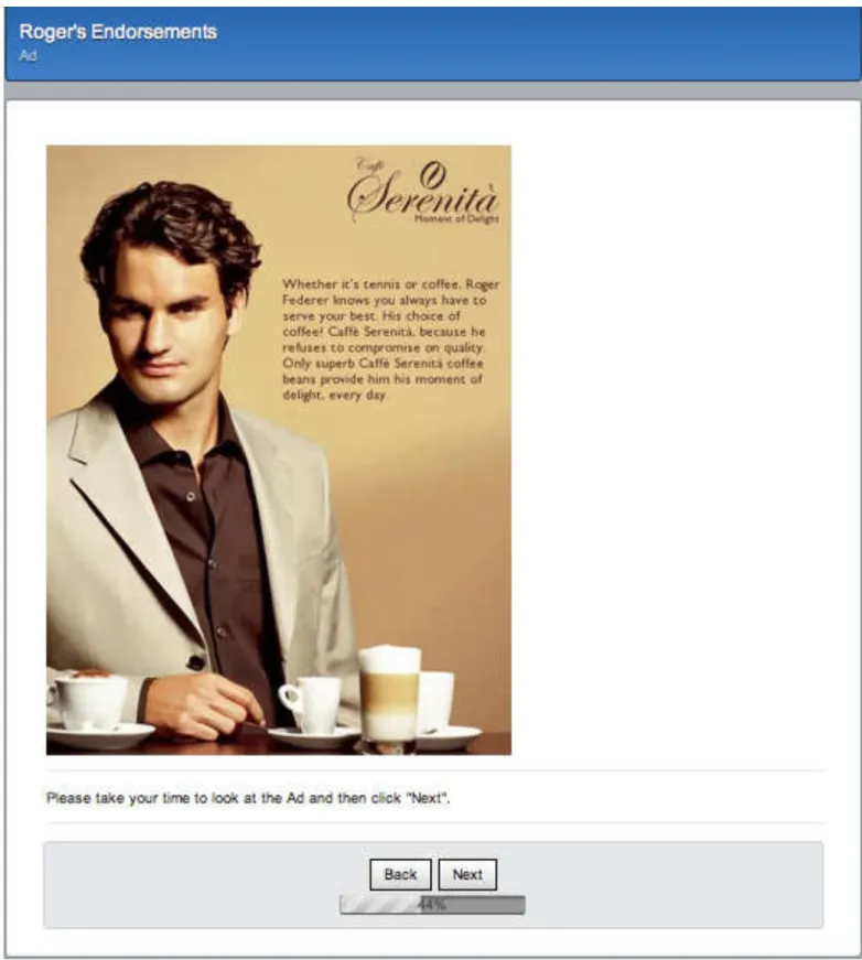
Figure 6: Example of Pretest 2, Ad

(12)

XII

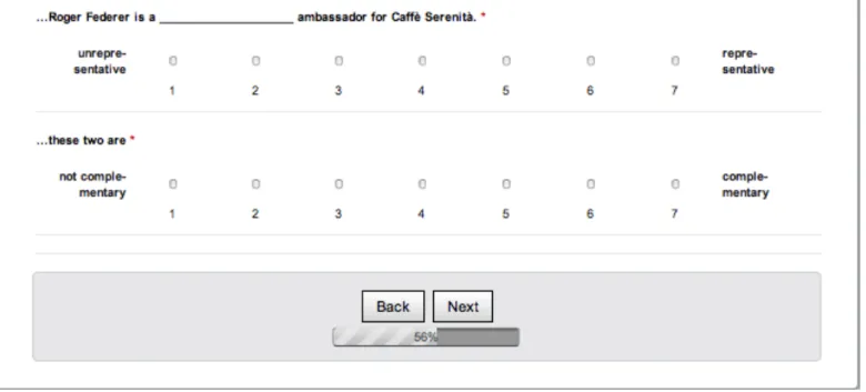
Figure 7: Example of Pretest 2, Evaluation of Fit

(13)

XIII

Figure 8: Continuing: Example of Pretest 2, Evaluation of Fit

Figures 4 to 8 illustrate parts of the survey of Pretest 2. Participants were introduced to Roger Federer (see Fig. 4) and to the coffee brand Caffè Serenità (see Fig. 5), they were shown an advertisement of Roger Federer endorsing Caffè Serenità (see Fig. 6) and were subsequently asked to evaluate the fit between the celebrity and the brand (see Figs. 7 and 8). Afterwards they were going through the same process when evaluating the fit between Roger Federer and the sports brand Halma.

Measures:

(14)

XIV Results

!"#$%&#"'() *+,!-.-(/.012 30,!-.-(/.012 !"## $"%& '"() %"## *"!$ '"+! *"## '"'+ )"() $"## %"$* '"## '"## )"+! )"'+ )"## )"## '"() +"## *"+! )"+! ("## +"## )"() &"## )"## )"%& !#"## *"+! '"() !!"## '"## )"## !%"## $"+! '"+! !*"## )"$* )"!$ !$"## $"## '"!$ !'"## %"!$ )"## !)"## '"+! )"$* !+"## )"## )"!$ !("## '"+! )"%& !&"## '"+! )"!$ %#"## '"!$ )"%& 4"5& 6789 97:8 Figure 9: Evaluations of Fit (N=20)

(15)

XV 6.3.1.3 Pretest 3

(16)

XVI

(17)

XVII

Figure 12: Example of Pretest 3, Evaluation of Fit

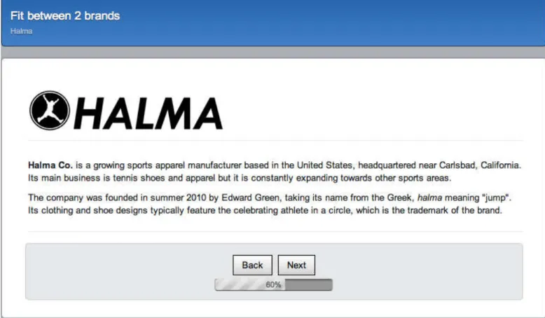
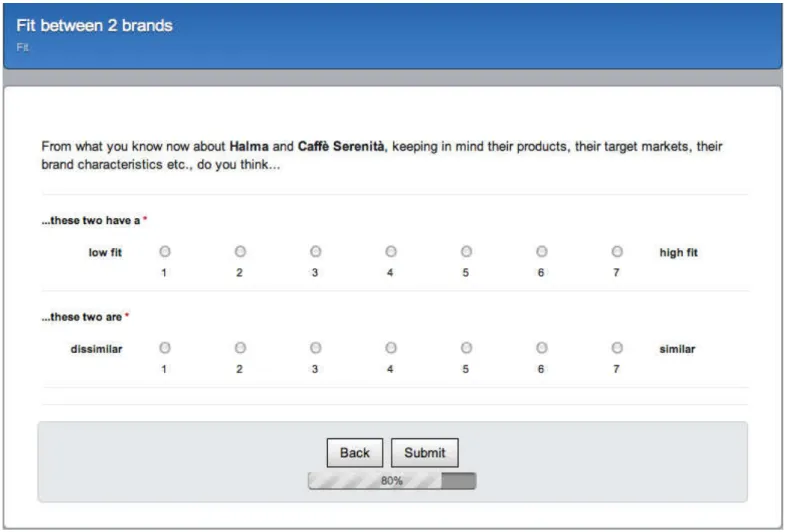
Figures 10 to 12 illustrate parts of the survey of Pretest 3. Participants were introduced to the coffee brand Caffè Serenità (see Fig. 10) and to the sports brand Halma (see Fig. 11), and subsequently were asked to evaluate the fit between the two brands (see Fig. 12).

Measures

Fit between Caffè Serenità and Halma was measured on 7-point semantic differential scales with 2 of 7 items (dissimilar/similar, low fit/high fit) that were used in a prior study of Simons and Becker-Olsen, 2006. Higher numbers on a scale represent a more positive evaluation of the fit and a participants’s evaluation of fit is composed of the average of the two scales measuring this variable.

(18)

XVIII Results !"#$%&#"'() *+,-.,/(0,.12 ! "#$ " " % "#$ & !#$ $ !#$ ' ! ( " ) % * "#$ !+ "#$ !! "#$ !" !#$ !% " !& ! !$ "#$ !' "#$ !( " !) % !* !#$ "+ "#$ 3"4& 567

Figure 13: Evaluation of Fit (N=20)

(19)

XIX 6.2.2 Final Survey

6.2.2.1 Groups 1 & 2

Figure 14: Final Survey, Groups 1 & 2, Introduction

(20)

XX

Figure 15: Final Survey, Groups 1 & 2, Instruction Celebrity and Brands

(21)

XXI

Figure 16: Final Survey, Groups 1 & 2, Roger Federer

(22)

XXII

Figure 17: Final Survey, Groups 1 & 2, Halma

(23)

XXIII

Figure 18: Final Survey, Groups 1 & 2, Ad I Halma

(24)

XXIV

(25)

XXV

(26)

XXVI

(27)

XXVII

(28)

XXVIII

(29)

XXIX

(30)

XXX

Figure 25: Final Survey, Group 1, Instruction Newspaper Article

(31)

XXXI

Figure 26: Final Survey, Group 1, Newspaper Article

(32)

XXXII

(33)

XXXIII

(34)

XXXIV

(35)

XXXV

(36)

XXXVI

(37)

XXXVII

(38)

XXXVIII

(39)

XXXIX

Figure 34: Final Survey, Groups 1 & 2, Thank You

Figures 14 to 34 illustrate the complete survey for group 1 (experimental group). Group 2’s survey looks exactly the same but does not include the newspaper article (see Fig. 26) as well as the instruction on the newspaper article (see Fig. 25).

(40)

XL 6.2.2.2 Groups 3 & 4

Figure 35: Final Survey, Groups 3 & 4, Introduction

(41)

XLI

(42)

XLII

(43)

XLIII

(44)

XLIV

(45)

XLV

Figure 40: Final Survey, Group 3, Newspaper Article

(46)

XLVI

(47)

XLVII

(48)

XLVIII

(49)

XLIX

(50)

L

Figure 45: Final Survey, Groups 3 & 4, Thank You

Figures 35 to 45 illustrate the complete survey for group 3. Group 4’s survey looks exactly the same but does not include the newspaper article (see Fig. 40) as well as the instruction on the newspaper article (see Fig. 39).

(51)

LI 6.3 SPSS Output

Explanation:

Markings

1. Red markings refer to the comparison of means between group 1 and group 2 2. Green markings refer to the comparison of means between group 3 and group 4. 3. Orange border lines refer to the comparison of means between group 1 and group 3.

4. Blue border lines refer to the comparison of means between group 2 and group 4.

5.!"#$%&'#$(')*+&',-"./&,'"&0&"'-1'-2&'/&"3&$-#%&'32#$%&'10'#--.-+(&'-14#"(,'5#*6#7

Variables

HA_ATTITUDE: Attitude toward Halma

RF_ATTITUDE: Attitude toward Roger Federer CS_ATTITUDE: Attitude toward Caffè Serenità

Groups Experimental Design Negative Article on Halma No Negative Article on Halma

Celebrity Group 1 Group 2

No Celebrity Group 3 Group 4

Figure 46: Overview of the Different Groups

(52)

LII 6.3.1 All Cases, N=435

6.3.1.a ANOVA (All Cases, N=435)

Figures 47-54 illustrate the data analysis on all respondents (N=435). A respondent’s attitude consists of the mean score of the scales measuring this variable.

Oneway

Filter <none> Lower Bound Upper Bound

1 105 2,838 1,3394 ,1307 2,579 3,097 1,0 6,2

2 122 5,179 1,0201 ,0924 4,996 5,362 1,6 6,8

3 117 2,460 1,2282 ,1135 2,235 2,685 1,0 6,0

4 91 4,585 ,8637 ,0905 4,405 4,764 2,6 7,0

Total 435 3,758 1,6271 ,0780 3,605 3,911 1,0 7,0

1 105 4,7524 1,57371 ,15358 4,4478 5,0569 1,00 7,00

2 122 5,7992 1,13802 ,10303 5,5952 6,0032 2,00 7,00

3 0 . . . .

4 0 . . . .

Total 227 5,3150 1,45143 ,09633 5,1251 5,5048 1,00 7,00

1 105 4,8214 1,25774 ,12274 4,5780 5,0648 1,00 7,00

2 122 5,1160 1,22918 ,11128 4,8957 5,3363 1,25 7,00

3 117 4,9774 1,13516 ,10495 4,7695 5,1852 2,00 7,00

4 91 5,1341 ,88094 ,09235 4,9506 5,3175 2,80 6,60

Total 435 5,0114 1,14932 ,05511 4,9031 5,1197 1,00 7,00

Descriptives

N Mean

Std.

Deviation Std. Error

95% Confidence Interval for Mean

Minimum Maximum HA_ATTITUDE

RF_ATTITUDE

CS_ATTITUDE

Notes

Figure 47: Descriptives (All Cases, N=435); Source: SPSS Output

Figure 47 shows important descriptives:

1. The means of the attitude toward Halma (HA_ATTITUDE), Roger Federer (RF_ATTITUDE) and Caffè Serenità (CS_ATTITUDE) of group 1 and group 2 are highlighted by the red markings.

a. Different evaluations of HA_ATTITUDE between group 1 and 2 are analyzed to prove H1.

b. Different evaluations of RF_ATTITUDE between group 1 and 2 are analyzed to prove H2a.

c. Different evaluations of CS_ATTITUDE between group 1 and 2 are analyzed to prove H2b. ⇒ For each of the three variables, the means in group 1 are lower than in group 2. These differences

(53)

LIII 2. The means of the attitude toward Caffè Serenità (CS_ATTITUDE) of group 3 and group 4 are

highlighted by the green markings.

a. Different evaluations of CS_ATTITUDE between group 3 and 4 are analyzed to prove H3. ⇒ This difference is not significant (see Figures 52 and 54).

3. The means of the attitude toward Halma (HA_ATTITUDE) of group 2 and group 4 are highlighted by the blue border lines.

a. Different evaluations of HA_ATTITUDE between group 2 and 4 are analyzed to show the positive impact a celebrity has on the attitude toward a brand.

⇒ The evaluations of group 2 (with endorsing celebrity) are higher than of group 4 (no endorsing celebrity). This mean difference is significant (see Figure52).

4. The means of the attitude toward Halma (HA_ATTITUDE) of group 1 and group 3 are highlighted by the orange border lines.

a. Different evaluations of HA_ATTITUDE between group 1 and 3 are analyzed to show the positive impact a celebrity has on the attitude toward a brand that is affected by negative publicity.

⇒ The evaluations of group 1 (with endorsing celebrity) are higher than of group 3 (no endorsing celebrity). This mean difference is significant (see Figure 52).

Group Mean Group Mean

2 5,179 4 4,585

1 2,838 3 2,460

%-Change -45,1966 %-Change -46,346

Figure 48: %-Changes of Attitude toward Halma (All Cases, N=435); Source: Own Illustration

(54)

LIV

⇒ The comparison reveals a less negative change between the groups that are endorsed by a celebrity (-45.20% vs. -46.35%).

In the following section the significances of the mean differences are tested.

Levene Statistic df1 df2 Sig.

HA_ATTITUDE 8,740 3 431 ,000

RF_ATTITUDE 18,456 1 225 ,000

CS_ATTITUDE 2,827 3 431 ,038

Test of Homogeneity of Variances

Figure 49: Test of Homogeneity (All Cases, N=435); Source: SPSS Output

Figure 49 shows the Levene-Test of homogeneity of variances. The test proves the null-hypothesis that the variances of the considered variable are universally equal in the groups. The significance shows the probability of making a mistake by rejecting the null-hypothesis.2

⇒ The test reveals that for each variable, this null-hypothesis has to be rejected since the significance is less than 0.05. Subsequently, equal variances cannot be assumed.

Sum of

Squares df

Mean

Square F Sig.

Between Groups 594,447 3 198,149 153,991 ,000

Within Groups 554,592 431 1,287

Total 1149,039 434

Between Groups 61,837 1 61,837 33,586 ,000

Within Groups 414,267 225 1,841

Total 476,104 226

Between Groups 6,629 3 2,210 1,681 ,170

Within Groups 566,657 431 1,315

Total 573,286 434

HA_ATTITUDE

RF_ATTITUDE

CS_ATTITUDE

ANOVA

Figure 50: ANOVA (All Cases, N=435); Source: SPSS Output

Figure 50 illustrates the outcome of the ANOVA. But since equal variances cannot be assumed, the requirements for this test are not satisfied.

(55)

LV

Statistica

df1 df2 Sig.

HA_ATTITUDE Welch 154,556 3 235,339 ,000

RF_ATTITUDE Welch 32,039 1 186,253 ,000

CS_ATTITUDE Welch 1,659 3 237,491 ,177

a. Asymptotically F distributed.

Robust Tests of Equality of Means

Figure 51: Welch Tests, (All Cases, N=435); Source: SPSS Output

Figure 51 shows the outcome of the Welch-Test. This test is run instead of an ANOVA, if equal variances in the groups cannot be assumed. For each variable it tests the null-hypothesis that the means of all four groups are equal. But to test the hypotheses it requires a comparison of only two respective groups. Since Roger Federer occurs only in group 1 and 2, the Welch-Test, in this case, can only compare the means of attitude toward Roger Federer of these two groups. In this way it is possible to test the significance of the mean difference between only group 1 and 2.

(56)

LVI

1 2 3 4

1 1 -1 0 0

2 0 0 1 -1

3 1 0 -1 0

4 0 1 0 -1

Value of

Contrast Std. Error t df

Sig. (2-tailed) 1 -2,341 ,1510 -15,500 431 ,000 2 -2,125 ,1585 -13,401 431 ,000

3 ,378 ,1525 2,481 431 ,013

4 ,594 ,1571 3,781 431 ,000

1 -2,341 ,1600 -14,625 192,517 ,000 2 -2,125 ,1452 -14,631 204,073 ,000 3 ,378 ,1731 2,185 211,967 ,030 4 ,594 ,1293 4,593 207,572 ,000 1 -1,0468 ,18063 -5,795 225 ,000 3 4,7524 ,13242 35,889 225 ,000 4 5,7992 ,12285 47,206 225 ,000 1 -1,0468 ,18494 -5,660 186,253 ,000 3 4,7524 ,15358 30,944 104,000 ,000 4 5,7992 ,10303 56,286 121,000 ,000 1 -,2946 ,15264 -1,930 431 ,054 2 -,1567 ,16027 -,978 431 ,329 3 -,1559 ,15414 -1,012 431 ,312 4 -,0181 ,15882 -,114 431 ,909 1 -,2946 ,16568 -1,778 218,407 ,077 2 -,1567 ,13979 -1,121 206,000 ,264 3 -,1559 ,16149 -,966 210,688 ,335 4 -,0181 ,14461 -,125 210,697 ,901 CS_ATTITUDE Assume equal

variances

Does not assume equal variances HA_ATTITUDE Assume equal

variances

Does not assume equal variances

RF_ATTITUDE Assume equal variances

Does not assume equal variances Contrast Coefficients Contrast Group Contrast Tests Contrast

Figure 52: Contrasts, (All Cases, N=435); Source: SPSS Output

Figure 52 shows the results of the contrast tests. A contrast test looks at differences in means of only two respective groups. It is very similar to a normal T-Test, but in the case of assumed equal variances, the contrast test uses the degrees of freedom of all the groups that are represented in the respective variable. The T-Test in comparison, only considers the degrees of freedom of the two compared groups. Additionally, the contrast test is based on a Levene-Test that tested the variances of all the groups that are represented in the respective variable. The Levene-Test aimed at the T-Test only considers the two compared groups.

(57)

LVII

⇒ The red markings show a significant difference in means between group 1 and 2 for HA_ATTITUDE (t(192.52) = -14.63, p < 0.001), RF_ATTITUDE (t(186.25) = -5.66, p < 0.001) and

CS_ATTITUDE (t(218.41) = -1.78, p < 0.05 (one-tailed)).

⇒ The green markings show no significant difference in means between group 3 and 4 for CS_ATTITUDE (t(206.00) = -1.12, p > 0.25).

⇒ The orange border lines show a significant difference in means between group 1 and 3 for HA_ATTITUDE (t(211.97) = 2.19, p < 0.05).

(58)

LVIII 6.3.1.b T-Tests (All Cases, N=435)

Figure 53: T-Tests, Group 1 & 2, (All Cases, N=435); Source: SPSS Output

(59)

LIX Figure 53 and 54 show the results of the T-Test.

CS_ATTITUDE (t(225) = -1.78, p < 0.05 (one-tailed)).

(60)

LX 6.3.2 Filter: Appropriateness, N=384

6.3.2.a ANOVA (Filter: Appropriateness, N=384)

Figures 55-62 illustrate the data analysis on respondents evaluating the endorsements as appropriate (N=385). A Respondent’s attitude consists of the mean score of the scales measuring this variable.

Oneway

Filter

Bound Bound

1 74 3,205 1,2902 ,1500 2,906 3,504 1,0 6,2

2 102 5,247 ,9297 ,0921 5,064 5,430 2,6 6,8

3 117 2,460 1,2282 ,1135 2,235 2,685 1,0 6,0

4 91 4,585 ,8637 ,0905 4,405 4,764 2,6 7,0

Total 384 3,847 1,5799 ,0806 3,689 4,006 1,0 7,0

1 74 5,1284 1,47539 ,17151 4,7866 5,4702 1,00 7,00

2 102 5,9387 1,03314 ,10230 5,7358 6,1417 2,50 7,00

3 0 . . . .

4 0 . . . .

Total 176 5,5980 1,29807 ,09785 5,4049 5,7911 1,00 7,00

1 74 5,0865 ,99162 ,11527 4,8567 5,3162 2,50 7,00

2 102 5,4299 ,89665 ,08878 5,2538 5,6060 3,00 7,00

3 117 4,9774 1,13516 ,10495 4,7695 5,1852 2,00 7,00

4 91 5,1341 ,88094 ,09235 4,9506 5,3175 2,80 6,60

Total 384 5,1557 1,00143 ,05110 5,0553 5,2562 2,00 7,00

(CS_APPROPRIATENESS >= 3 OR MISSING (CS_APPROPRIATENESS)) AND (HA_APPROPRIATENESS >= 3 OR MISSING (HA_APPROPRIATENESS)) (FILTER) HA_ATTITUDE RF_ATTITUDE CS_ATTITUDE Notes Descriptives N Mean Std.

95% Confidence

Minimum Maximum

Figure 55: Descriptives (Filter: Appropriateness, N=384); Source: SPSS Output

c. Different evaluations of CS_ATTITUDE between group 1 and 2 are analyzed to prove H2b. ⇒ For each of the three variables, the means in the group 1 are lower than in group 2. These

(61)

LXI 2. The means of the attitude toward Caffè Serenità (CS_ATTITUDE) of group 3 and group 4 are

2 5,247 4 4,585

1 3,205 3 2,460

%-Change -38,9104 %-Change -46,346

Figure 56: %-Changes of Attitude toward Halma (Filter: Appropriateness, N=384); Source: Own Illustration

(62)

LXII

HA_ATTITUDE 7,736 3 380 ,000

RF_ATTITUDE 13,343 1 174 ,000

CS_ATTITUDE 3,176 3 380 ,024

Figure 57: Test of Homogeneity (Filter: Appropriateness, N=384); Source: SPSS Output

⇒ The test reveals that for each variable, this null-hypothesis has to be rejected since the significance is less than 0.05. Subsequently, equal variances cannot be assumed.

Sum of

Squares df

Mean

Square F Sig.

Between Groups 505,046 3 168,349 141,867 ,000

Within Groups 450,932 380 1,187

Total 955,977 383

Between Groups 28,162 1 28,162 18,373 ,000

Within Groups 266,710 174 1,533

Total 294,872 175

Between Groups 11,788 3 3,929 4,010 ,008

Within Groups 372,305 380 ,980

Total 384,092 383

HA_ATTITUDE

RF_ATTITUDE

CS_ATTITUDE

ANOVA

Figure 58: ANOVA (Filter: Appropriateness, N=384); Source: SPSS Output

Figure 58 illustrates the outcome of the ANOVA. But since equal variances cannot be assumed, the requirements for this test are not satisfied.

(63)

LXIII

Statistica _df1 _df2 _Sig.

a. Asymptotically F distributed.

Figure 59: Welch Tests (Filter: Appropriateness, N=384); Source: SPSS Output

⇒ The significance of RF_ATTITUDE shows that there is a significant difference in the means between group 1 and group 2 with p < 0.001 (F(1,122.93) = 16.47, p < 0.001).

(64)

LXIV

1 2 3 4

1 1 -1 0 0

2 0 0 1 -1

3 1 0 -1 0

4 0 1 0 -1

Value of

Sig. (2-tailed) 1 -2,042 ,1663 -12,274 380 ,000 2 -2,125 ,1523 -13,955 380 ,000

3 ,746 ,1618 4,608 380 ,000

4 ,662 ,1571 4,217 380 ,000

1 -2,042 ,1760 -11,602 125,485 ,000 2 -2,125 ,1452 -14,631 204,073 ,000 3 ,746 ,1881 3,963 149,710 ,000 4 ,662 ,1291 5,131 190,678 ,000 1 -,8103 ,18905 -4,286 174 ,000 3 5,1284 ,14392 35,633 174 ,000 4 5,9387 ,12259 48,445 174 ,000 1 -,8103 ,19970 -4,058 122,932 ,000 3 5,1284 ,17151 29,901 73,000 ,000 4 5,9387 ,10230 58,054 101,000 ,000 1 -,3434 ,15115 -2,272 380 ,024 2 -,1567 ,13835 -1,133 380 ,258

3 ,1091 ,14702 ,742 380 ,458

4 ,2958 ,14273 2,073 380 ,039

1 -,3434 ,14550 -2,360 147,722 ,020 2 -,1567 ,13979 -1,121 206,000 ,264 3 ,1091 ,15589 ,700 170,465 ,485 4 ,2958 ,12810 2,309 189,215 ,022 CS_ATTITUDE Assume equal

variances

Does not assume equal variances HA_ATTITUDE Assume equal

variances

RF_ATTITUDE Assume equal variances

Contrast Coefficients

Contrast Group

Contrast Testsa

Contrast

Figure 60: Contrasts (Filter: Appropriateness, N=384); Source: SPSS Output

Therefore results might differ slightly to the results of the T-Test, introduced in paragraph G.

(65)

LXV

⇒ The orange border lines show a significant difference in means between group 1 and 3 for HA_ATTITUDE (t(149.71) = 3.96, p < 0.001)

⇒ The blue border lines show a significant difference in means between group 2 and 4 for HA_ATTITUDE

(66)

LXVI 6.3.2.b T-Tests (Filter: Appropriateness, N=384)

T-Test N Mean Std. Deviation Std. Error Mean

1 74 3,205 1,2902 ,1500

2 102 5,247 ,9297 ,0921

1 74 5,1284 1,47539 ,17151

2 102 5,9387 1,03314 ,10230

1 74 5,0865 ,99162 ,11527

2 102 5,4299 ,89665 ,08878

Lower Upper

Equal variances assumed

9,653 ,002 -12,205 174 ,000 -2,0417 ,1673 -2,3718 -1,7115

Equal variances not assumed

-11,602 125,485 ,000 -2,0417 ,1760 -2,3899 -1,6934

13,343 ,000 -4,286 174 ,000 -,81035 ,18905 -1,18348 -,43721

-4,058 122,932 ,000 -,81035 ,19970 -1,20565 -,41505

,786 ,376 -2,398 174 ,018 -,34342 ,14318 -,62601 -,06082

-2,360 147,722 ,020 -,34342 ,14550 -,63094 -,05589

CS_ATTITUDE HA_ATTITUDE

RF_ATTITUDE

Levene's Test for

Equality of Variances t-test for Equality of Means

Mean Difference

Std. Error Difference

95% Confidence Interval of the

Difference CS_ATTITUDE

Independent Samples Test

F Sig. t df

Group Statistics Group HA_ATTITUDE RF_ATTITUDE Sig. (2-tailed)

Figure 61: T-Test, Group 1 & 2, (Filter: Appropriateness, N=384); Source: SPSS Output

N Mean Std. Deviation Std. Error Mean

3 117 4,9774 1,13516 ,10495

4 91 5,1341 ,88094 ,09235

Lower Upper

6,823 ,010 -1,087 206 ,278 -,15672 ,14422 -,44105 ,12762

-1,121 206,000 ,264 -,15672 ,13979 -,43232 ,11889

CS_ATTITUDE t df Sig. (2-tailed) Mean Difference Std. Error Difference Sig. 95% Confidence Interval of the

Difference Group Statistics

Group

CS_ATTITUDE

Levene's Test for t-test for Equality of Means

F

(67)

LXVII Figure 61 and 62 show the results of the T-Test.

CS_ATTITUDE (t(174) = -2.40, p < 0.05).

(68)

LXVIII 6.3.3 Filter: Germany, N=181

6.3.3.a ANOVA (Filter: Germany, N=181)

Figures 63-70 illustrate the data analysis on all respondents from Germany (N=181). A Respondent’s attitude consists of the mean score of the scales measuring this variable.

Oneway

Filter Lower Bound Upper Bound

1 46 3,035 1,1565 ,1705 2,691 3,378 1,2 5,6

2 45 4,902 1,0204 ,1521 4,596 5,209 2,0 6,8

3 44 2,391 1,0547 ,1590 2,070 2,712 1,0 5,2

4 46 4,335 ,7900 ,1165 4,100 4,569 2,6 6,0

Total 181 3,673 1,4164 ,1053 3,465 3,881 1,0 6,8

1 46 4,5435 1,72667 ,25458 4,0307 5,0562 1,00 7,00

2 45 5,7611 1,17980 ,17587 5,4067 6,1156 2,50 7,00

3 0 . . . .

4 0 . . . .

Total 91 5,1456 1,59560 ,16726 4,8133 5,4779 1,00 7,00

1 46 4,5435 1,22622 ,18080 4,1793 4,9076 1,00 7,00

2 45 5,0967 1,15352 ,17196 4,7501 5,4432 2,00 7,00

3 44 5,0284 1,08265 ,16322 4,6993 5,3576 2,50 7,00

4 46 4,8957 ,69377 ,10229 4,6896 5,1017 3,60 6,60

Total 181 4,8884 1,07124 ,07962 4,7313 5,0455 1,00 7,00

Country = "Germany" (FILTER)

HA_ATTITUDE RF_ATTITUDE CS_ATTITUDE Notes Descriptives N Mean Std.

95% Confidence

Minimum Maximum

Figure 63: Descriptives (Filter: Germany, N=181); Source: SPSS Output

c. Different evaluations of CS_ATTITUDE between group 1 and 2 are analyzed to prove H2b. ⇒ For each of the three variables, the means in group 1 are lower than in group 2. These differences

(69)

LXIX 2. The means of the attitude toward Caffè Serenità (CS_ATTITUDE) of group 3 and group 4 are

2 4,902 4 4,335

1 3,035 3 2,391

%-Change -38,0937 %-Change -44,8436

Figure 64: %-Changes of Attitude toward Halma (Filter: Germany, N=181); Source: Own Illustration

(70)

LXX

HA_ATTITUDE 2,175 3 177 ,093

RF_ATTITUDE 9,123 1 89 ,003

CS_ATTITUDE 4,844 3 177 ,003

Figure 65: Test of Homogeneity (Filter: Germany, N=181); Source: SPSS Output

⇒ The test reveals that for RF_ATTITUDE and CS_ATTITUDE, this null-hypothesis has to be rejected since the significance is less than 0.05. Subsequently, equal variances cannot be assumed for these variables. For HA_ATTITUDE on the other hand, equal variances can be assumed, since the significance is above 0.05.

(71)

LXXI

Sum of

Squares df

Mean

Square F Sig.

Between Groups 179,203 3 59,734 58,120 ,000

Within Groups 181,915 177 1,028

Total 361,117 180

Between Groups 33,726 1 33,726 15,361 ,000

Within Groups 195,407 89 2,196

Total 229,133 90

Between Groups 8,289 3 2,763 2,467 ,064

Within Groups 198,271 177 1,120

Total 206,561 180

HA_ATTITUDE

RF_ATTITUDE

CS_ATTITUDE

ANOVA

Figure 66: ANOVA (Filter: Germany, N=181); Source: SPSS Output

Figure 66 illustrates the outcome of the ANOVA. This test requires assumed equal variances, which is given only for HA_ATTITUDE. For this variable, the test proves if the means of all four groups are significantly different from each other. Therefore it is irrelevant for this study.

Statistica df1 df2 Sig.

Figure 67: Welch Tests (Filter: Germany, N=181); Source: SPSS Output

⇒ The significance of RF_ATTITUDE shows that there is a significant difference in the means between group 1 and group 2 with p < 0.001 (F(1,79.65) = 15.49, p < 0.001).

(72)

LXXII

1 2 3 4

1 1 -1 0 0

2 0 0 1 -1

3 1 0 -1 0

4 0 1 0 -1

Value of

Sig. (2-tailed) 1 -1,867 ,2126 -8,785 177 ,000 2 -1,944 ,2138 -9,093 177 ,000

3 ,644 ,2138 3,012 177 ,003

4 ,567 ,2126 2,670 177 ,008

1 -1,867 ,2285 -8,173 88,075 ,000 2 -1,944 ,1971 -9,862 79,622 ,000 3 ,644 ,2331 2,762 87,806 ,007 4 ,567 ,1916 2,962 82,871 ,004 1 -1,2176 ,31068 -3,919 89 ,000 3 4,5435 ,21847 20,797 89 ,000 4 5,7611 ,22089 26,082 89 ,000 1 -1,2176 ,30943 -3,935 79,648 ,000 3 4,5435 ,25458 17,847 45,000 ,000 4 5,7611 ,17587 32,757 44,000 ,000 1 -,5532 ,22191 -2,493 177 ,014

2 ,1328 ,22318 ,595 177 ,553

3 -,4849 ,22318 -2,173 177 ,031

4 ,2010 ,22191 ,906 177 ,366

1 -,5532 ,24951 -2,217 88,866 ,029 2 ,1328 ,19262 ,689 72,696 ,493 3 -,4849 ,24357 -1,991 87,451 ,050 4 ,2010 ,20008 1,005 71,852 ,318 RF_ATTITUDE Assume equal

variances

CS_ATTITUDE Assume equal variances

Contrast Group

Contrast Testsa

Contrast

HA_ATTITUDE Assume equal variances

Contrast Coefficients

Figure 68: Contrasts (Filter: Germany, N=181); Source: SPSS Output

Therefore results might differ slightly to the results of the T-Test, introduced in paragraph G.

⇒ The red markings show a significant difference in means between group 1 and 2 for HA_ATTITUDE (t(177) = -8.79, p < 0.001), RF_ATTITUDE (t(79.65) = -3.94, p < 0.001) and

(73)

LXXIII

⇒ The green markings show no significant difference in means between group 3 and 4 for CS_ATTITUDE (t(72.70) = 0.69, p > 0.45).

⇒ The orange border lines show a significant difference in means between group 1 and 3 for HA_ATTITUDE (t(177) = 3.01, p < 0.005).

⇒ The blue border lines show a significant difference in means between group 2 and 4 for HA_ATTITUDE (t(177) = 2.67, p < 0.01).

(74)

LXXIV 6.3.3.b T-Tests (Filter: Germany, N=181)

T-Test N Mean Std. Deviation Std. Error Mean

1 46 3,035 1,1565 ,1705

2 45 4,902 1,0204 ,1521

1 46 4,5435 1,72667 ,25458

2 45 5,7611 1,17980 ,17587

1 46 4,5435 1,22622 ,18080

2 45 5,0967 1,15352 ,17196

Lower Upper

,322 ,572 -8,161 89 ,000 -1,8674 ,2288 -2,3221 -1,4128

-8,173 88,075 ,000 -1,8674 ,2285 -2,3215 -1,4134

9,123 ,003 -3,919 89 ,000 -1,21763 ,31068 -1,83494 -,60032

-3,935 79,648 ,000 -1,21763 ,30943 -1,83345 -,60181

,002 ,968 -2,216 89 ,029 -,55319 ,24968 -1,04930 -,05708

-2,217 88,866 ,029 -,55319 ,24951 -1,04898 -,05740

CS_ATTITUDE Sig. (2-tailed) Mean Difference Std. Error Difference 95% Confidence Interval of the

Difference

HA_ATTITUDE

RF_ATTITUDE CS_ATTITUDE

Levene's Test for

Equality of Variances t-test for Equality of Means

F Sig. t df

Group Statistics

Group

HA_ATTITUDE

RF_ATTITUDE

Figure 69: T-Test, Group 1 & 2, (Filter: Germany, N=181); Source: SPSS Output

N Mean

Std. Deviation

Std. Error Mean

3 44 5,0284 1,08265 ,16322

4 46 4,8957 ,69377 ,10229

Lower Upper

9,630 ,003 ,696 88 ,488 ,13276 ,19082 -,24646 ,51197

,689 72,696 ,493 ,13276 ,19262 -,25116 ,51668

95% Confidence Interval of the

Difference Group Statistics

Group

CS_ATTITUDE

Levene's Test for t-test for Equality of Means

F CS_ATTITUDE t df Sig. (2-tailed) Mean Difference Std. Error Difference Sig.

(75)

LXXV Figure 69 and 70 show the results of the T-Test.

⇒ The red markings show a significant difference in means between group 1 and 2 for HA_ATTITUDE (t(89) = -8.16, p < 0.001), RF_ATTITUDE (t(79.65) = -3.94, p < 0.001) and

CS_ATTITUDE (t(89) = -2.22, p < 0.05).