Optimal design of a plate of variable thickness:
a variational approach in dimension one
PABLO PEDREGAL and ALBERTO DONOSO
ETSI Industriales, Universidad de Castilla-La Mancha 13071 Ciudad Real, Spain
E-mail: [email protected]
Abstract. For a typical design problem of a plate of variable thickness, we analyze the one-dimensional situation through a variational reformulation to discover that, in contrast with the higher dimensional case, there are optimal solutions. Another typical interpretation of this simpli-fication is that of the optimal shape of a bending beam. The mechanism employed for the existence issue is the direct method for the new formulation. Optimality conditions are then pursued. Mathematical subject classification:49J15, 49J45, 49K15, 74K20, 74P05. Key words:periodic plate, optimal design, direct method, optimality conditions.
1 Introduction
In this paper, we analyze a simplified, one-dimensional model for the optimal design of a plate of variable thickness which is assumed to be infinite along one of its axes. In general, the Kirchhoff model for pure bending of symmetric plates ([5], [9]) postulates that the deflection of vertical displacementwof a plate is the solution of the fourth order, elliptic equation
i,j,k,l
∂2 ∂xi∂xj
Mij kl
∂2w ∂xk∂x1
=F in,
whereF ∈L2()is the vertical load,is the midplane of the plate with respect to which the plate is symmetric, and the design of the plate lies in the tensorM
M = 2
3h
3(x)B (1.1)
wherehis the half-thickness andBis the tensor of material constants. Boundary conditions for a clamped plate incorporate
w= ∂w
∂n =0 on∂.
Under the assumptions that=(0,1)×(0,1), bothhandF depend only on
x1, and if we replace the boundary conditionw = 0 onx2 = 0,x2 = 1, by a periodic boundary condition, it is elementary to check that
w(x1, x2)=y(x1)
is the solution of the above problem wherey(x),x =x1, solves
2 3h
3(x)B
1111y′′(x) ′′
=F in(0,1), y(0)=y(1)=y′(0)=y′(1)=0.
Under these circumstances, the objective is to design the plate, i.e. to choose the functionh(x), so that we maximize the overall rigidity of the plate. A way of measuring this global rigidity is through the compliance functional
J (h)=
1 0
F (x)y(x) dx
which represents the work done by the loadF. Hence, maximum global rigidity corresponds to minimum compliance.
Further natural constraints on the feasible designs limit the amount of material to be used
0< h− ≤h(x)≤h+,
1 0
h(x) dx≤V ,
whereh−,h+andV are positive constants given in a coherent way
h−< V < h+.
Altogether, and given positive constants h− < V < h+, B = B1111 and
F ∈L2(0,1), we seek to
Minimize J (h)= 1
0
where
2 3h
3(x)By′′(x)
′′
=F in(0,1), y(0)=y(1)=y′(0)=y′(1)=0,
andhis feasible as specified in the last paragraph. Notice that the constants 2/3 andBcan be incorporated either in the designhor in the loadF so that we will look at the somewhat simpler problem
Minimize J (h)= 1
0
F (x)y(x) dx
subject to
h3(x)y′′(x)′′ =F in(0,1), y(0)=y(1)=y′(0)=y′(1)=0,
andhis such that
0< h−≤h(x)≤h+,
1 0
h(x) dx ≤V .
This type of optimal design problems have been analyzed in a number of papers (in addition to the references already cited see [4]) even in the two dimensional situation but the design still depending on one variable. One of the main features of these problems is the lack of optimal designs and the infinitesimal spatial oscillations leading to optimality. In the present work, and as a previous step to the higher dimensional situation, we pretend to recast the above optimal control problem in a purely variational format that may allow a treatment in the context of the Calculus of Variations by using all the tools and techniques of this discipline. This perspective have already been explored in [2] for one-dimensional situations and first order problems and, for instance, in [12] for vector, higher dimensional problems.
how our results can be adapted to treat a somewhat more general situation where we replace the third power occuring in (1.1) by a non-vanishing real powers.
The main contribution here is the somewhat surprising result, contrary to the higher dimensional situation ([3], [11]), that optimal designs exist. It is however true that existence of optimal solutions in simplified one-dimensional situations occurs in a variety of situations (see for instance [1], [7], [10]). This existence (Section 3) is achieved by a suitable reformulation as a variational problem (Section 2) to which classical techniques can be applied. In the final sections, optimality conditions are also explored and numerical implementations based on optimality are shown.
2 A variational reformulation
Letf be a primitive of a primitive ofF, i.e.
f (x)=
x
0 t
0
F (s) ds dt,
then the differential law can be reinterpreted by writing
h(x)sy′′(x)=f (x)+l(x) (2.1)
wherel(x)is a linear function in(0,1). The underlying idea for our reformulation is to consider (2.1) as a substitute of the differential equation and as a way to relate the pairs(y, l)with the designh. In addition, by performing an integration by parts twice on the cost functional and bearing in mind the boundary conditions ony, it is straightforward to realize
J (h)=
1 0
f (x)y′′(x) dx,
or even further
J (h)=
1 0
(f (x)+l(x)) y′′(x) dx
for any linear functionl(x). More precisely, consider the set
=(x, λ, ξ )∈R3:hsξ =f (x)+λfor someh∈ [h−, h+]
and define the density
ϕ:→R∗=R∪ {+∞}
by setting
ϕ(x, λ, ξ )=
(f (x)+λ)ξ, (x, λ, ξ )∈,
+∞, else.
The cost functional for the equivalent variational problem will be
I (l, y)= 1
0
ϕ(x, l(x), y′′(x)) dx
wherey ∈H2(0,1), it complies with all the boundary conditions andlis linear. The volume restriction, however, poses some difficulties. Indeed, solving forh
in (2.1) leads us to impose 1
0
f (x)+l(x)
y′′(x)
1/s
dx≤V .
For convenience, let us put
ψ (x, λ, ξ )=
f (x)+λ
ξ
1/s
, (x, λ, ξ )∈,
+∞, else.
If the set wheref equals a linear function is not negligible, the definition of
forcesy′′ to vanish in that same set, and thenhcan be chosen arbitrarily on
the admissible interval [h−, h+]. But that set does not contribute to the cost
functional (f′′ = 0) so that we would use as little material as we would be
allowed, i.e. we would chooseh(x)=h−in that set. This possibility has to be
compared with other choices when looking for optimal profiles.
Theorem 2.1. Our original optimal design problem is equivalent to the varia-tional problem
Minimize I (l, y)= 1
0
subject to
l, linear, y ∈H2(0,1), y(0)=y(1)=y′(0)=y′(1)=0,
1 0
ψ (x, l(x), y′′(x)) dx ≤V ,
in the sense that for any given feasible designh, there exists a feasible pair(l, y), and for any such given admissible pair(l, y)there is an admissible designh, such thatJ (h) = I (l, y). In particular the passage from optimal solutions of one problem to optimal solutions of the other is given by
h(x)=
f (x)+l(x)
y′′(x)
1/s
.
The proof has almost been indicated, and as a matter of fact, the new variational principle has been set up so that this equivalence is guaranteed.
We would like to clarify the existence-nonexistence of optimal solutions through the analysis of this equivalent variational problem by using the classical tool of the direct method.
3 Existence of optimal solutions
It is well-known that there are two main ingredients in the direct method of the Calculus of Variations in order to show existence of optimal solutions: weak lower semicontinuity and coercivity ([8]). Moreover weak lower semicontinuity is equivalent to convexity of the functionals involved in those variables where we have weak but not strong convergence ([13]). We treat those two issues succesively.
We first elucidate the weak lower semicontinuity property for our variational problem. This essentially involves the convexity of the functionsϕandψwith respect toξ. Notice that the weak convergence
lj ⇀ l inL2(0,1)
Lemma 3.1. The functionϕ(x, λ, ξ )is convex with respect toξ for any value ofs whileψ (x, λ, ξ )is convex with respect toξ provideds ≥ −1.
Proof. The proof consists in the realization that the set where bothϕandψare finite, i.e. the set, is convex inξ for fixed(x, λ). In fact
(x, λ)= {ξ ∈R:(x, λ, ξ )∈}
can be given explicitly as the interval with end-points
f (x)+λ
hs− and
f (x)+λ
hs+ .
In any case this is indeed a convex set. In addition, on such interval the functions
ϕandψare convex. On the one hand,ϕis even linear. On the other,ψis convex ifs ≥ −1 because in f (x)+λandξ must have the same sign.
The weak lower semicontinuity is a direct consequence of the convexity shown in the lemma. This is a standard fact.
Proposition 3.2. The functionals with integrandsϕandψare weak lower semi-continuous with respect to weak convergence inL2(0,1)×H2(0,1). Namely, if
lj →l inL2(0,1), yj ⇀ y inH2(0,1),
then
lim inf j→∞
1 0
ϕ(x, lj(x), y′′j(x)) dx ≥ 1
0
ϕ(x, l(x), y′′(x)) dx,
lim inf j→∞
1 0
ψ (x, lj(x), yj′′(x)) dx≥ 1
0
ψ (x, l(x), y′′(x)) dx.
Coercivity is another main ingredient for the success of the direct method in providing optimal solutions. In our situation, this is immediate because
hs−ξ2≤(f (x)+λ) ξ
if(x, λ, ξ )∈. Concerning coercivity forλit is also elementary to obtain
h2s−ξ
2
≤ |f (x)+λ|2
if(x, λ, ξ ) ∈ . The following theorem is a rather routine application of the
Theorem 3.3. Our variational problem admits optimal solutions if s ≥ −1, and consequently, so does our original optimal design problem.
4 Optimality conditions
Once the existence of optimal solutions has been rigorously established, we are entitled to pursue the analysis of optimality conditions in order to better understand the features of optimal solutions. Since the analysis that follows does not depend on the particular value ofsas long ass >0 and the values =3 is particularly important, we have restrict our computations in this section to this values =3, though the same calculations are valid for any such value ofs.
It turns out that the best way we have found to write optimality conditions down is to go back to the genuine design variablehbut keeping the variational form of the problem. In particular we still use (2.1) to write
y′′(x)= f (x)+l(x)
h3(x) ,
and thus eliminate the variabley′′from the variational form of the problem. It is
elementary to check that in this way we can write the problem in a new equivalent form as
Minimize 1
0
f (x)f (x)+l(x)
h3(x) dx
subject to
1 0
f (x)+l(x)
h3(x) dx=0,
1 0
xf (x)+l(x)
h3(x) dx=0,
1 0
h(x) dx ≤V ,
h− ≤h(x)≤h+.
These two new integral constraints come from the fact that
y′′(x)= f (x)+l(x)
must comply with the boundary conditions
y(0)=y(1)=y′(0)=y′(1)=0.
If we consider the conditionl′′ =0 as a “state equation" regardinglas the state
andhas the control, it is elementary to apply Pontryaguin’s maximum principle to obtain optimality conditions. Indeed, if we let
l1=l, l2=l′, l1′ =l2, l2′ =0, the hamiltonian is
H (x, l1, l2, p1, p2, h)=
(f (x)+l1(x))(f (x)+λ1+λ2x)
h3 +λ3h+p1l2,
where multipliersλiare associated with the three integral constraints andλ3≥0. Indeedλ3 > 0 is expected because the optimalhwill yield maximum volume
V. The dynamics for the costatespi are governed by
p1′ = −(f (x)+λ1+λ2x)
h3 , p
′
2= −p1, together with the transversality conditions
p1(0)=p1(1)=p2(0)=p2(1)=0. Therefore we can write
p1(x)= −
x
0
(f (t )+λ1+λ2t )
h(t )3 dt
and demand
1 0
(f (t )+λ1+λ2t )
h(t )3 dt =0. (4.1)
Likewise
p2(x)= x
0 s
0
(f (t )+λ1+λ2t )
h(t )3 dt ds,
1 0
s
0
(f (t )+λ1+λ2t )
Integrating by parts in this last integral and bearing in mind (4.1), we conclude 1
0
t(f (t )+λ1+λ2t )
h(t )3 dt =0. (4.2)
(4.1) and (4.2) imply thatl1(x)=λ1+λ2x. Therefore the remaining optimality condition enforcesh(x)to be the point of attainment of the minimum
min h−≤h≤h+
(f (x)+l1(x))2
h3 +λ3h
. (4.3)
This together with the three integral constraints 1
0
f (x)+l1(x)
h3(x) dx=0,
1 0
xf (x)+l1(x)
h3(x) dx=0,
1 0
h(x) dx=V ,
(4.4)
determines uniquely the optimalh(x) andl1(x), and the multiplier λ3. Even further if we put
γ (t )=
t, h−≤t≤h+,
h−, t≤h−,
h+, t≥h+,
then
h(x)=γ (3/λ3)1/4
|f (x)+l1(x)|
.
This information already yields interesting qualitative properties about optimal designs and how they can be found. If we rewrite this last formula in terms of
g(x)=
3
λ3 1/2
(f (x)+l1(x)) , we see that
where 1
0
g(x)
h(x)3dx=
1 0
x g(x)
h(x)3dx=0,
1 0
γ|g(x)|dx=V .
Notice thatF =(λ3/3)1/2g′′(x)implies thatgis smooth. In particular, we see that in the regionh−< h(x) < h+,hmust be the square root ofg. For instance,
ifF is constant, then transition fromh− toh+ must take place by arcs of the
square root. We will see this behavior in the numerical computations of the next section. These computations are based on the optimality information in this section.
5 Numerical computations
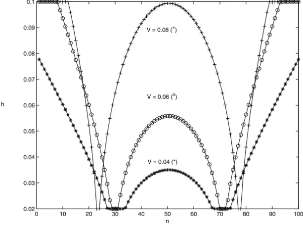
The numerical simulations that follow have been implemented by using in an elementary way the equilibrium conditions (4.3) and (4.4). The algorithm used is an elementary fixed point scheme transforming the multipliersλi,i =1,2,3, by utilizing (4.4). We have chosen two typical load regimes: the uniformly distributed constant load and the point Dirac delta load. Several simulations have been conducted in each case
1. for different values of the volumeV; 2. for different values ofh−;
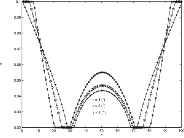
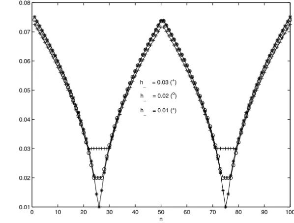
3. for different values of the powers.
For the uniform distributed constant vertical loadF, numerical results appear in Figures 1, 2, and 3, for the varying volume, varyingh−and different powers
s, respectively.
For the point Dirac delta load situated in the middle point of the beam, numer-ical optimal profiles, for the same three above situations, appear in Figures 4, 5, and 6.
6 Acknowledgements
0 10 20 30 40 50 60 70 80 90 100 0.02
0.03 0.04 0.05 0.06 0.07 0.08 0.09 0.1
n h
V = 0.08 (+)
V = 0.06 (o)
V = 0.04 (*)
Figure 1 – Optimal profile for different values ofV.
0 10 20 30 40 50 60 70 80 90 100
0.01 0.02 0.03 0.04 0.05 0.06 0.07 0.08 0.09 0.1
n h
h
_ = 0.03 ( +)
h
_ = 0.02 ( o)
h
_ = 0.01 (*)
0 10 20 30 40 50 60 70 80 90 100 0.02
0.03 0.04 0.05 0.06 0.07 0.08 0.09 0.1
n h
s = 3 (+) s = 2 (o) s = 1 (*)
Figure 3 – Optimal profile for different powerss.
0 10 20 30 40 50 60 70 80 90 100
0.02 0.03 0.04 0.05 0.06 0.07 0.08 0.09 0.1
n h
V = 0.08 (+)
V = 0.06 (o)
V = 0.04 (*)
0 10 20 30 40 50 60 70 80 90 100 0.01
0.02 0.03 0.04 0.05 0.06 0.07 0.08
n h
h
_ = 0.03 ( +)
h_ = 0.02 (o) h_ = 0.01 (*)
Figure 5 – Optimal profile for different values ofh−
0 10 20 30 40 50 60 70 80 90 100
0.02 0.03 0.04 0.05 0.06 0.07 0.08 0.09 0.1
n h
s = 3 (+) s = 2 (o) s = 1 (*)
REFERENCES
[1] Barnes, D.C.,Extremal problems for eigenvalues functionals, SIAM J. Math. Anal.,19(1988), 1151–1161.
[2] Bellido, J.C. and Pedregal, P.,Optimal design via variational principles: the one-dimensional case, J. Math. Pures Appl.,80(2001), 245–261.
[3] Bonnetier, E. and Conca, C., Relaxation totale d’un problème d’optimisation de plaques, CRAS Paris,317(1993), 931–936.
[4] Bonnetier, E. and Conca, C.,Approximation of Young measures by functions and application to a problem of optimal design for plates with variable thickness, Proc. Roy. Soc. Edin., A,
124(1994), 399–422.
[5] Bonnetier, E. and Vogelius, M.,Relaxation of a compliance functional for a plate optimiza-tion problem, Applications of Multiple Scaling in Mechanics, (P.G. Ciarlet and E. Sánchez-Palencia, eds.), Masson, 31-53, (1987).
[6] Bratus, A.S. and Posvyanskii, V.P.,The optimum shape of a bending beam, J. Appl. Maths. Mechs.,64(2000), 993–1004.
[7] Cox, S. and Overton, M.,On the optimal design of columns against buckling, SIAM J. Math. Anal.,23(1992), 287–325.
[8] Dacorogna, B.,Direct methods in the Calculus of Variations, Springer, (1989).
[9] Kohn, R.V. and Vogelius, M.,Thin plates with varying thickness, and their relation to structural optimization, Homogenization and Effective Moduli of Materials and Media, IMA Volumes 1, (Ericksen, J., Kinderlehrer, D., Kohn, R., Lions, J.L., eds), Springer-Verlag, 126-149, (1986).
[10] Muñoz, J., (submitted).
[11] Muñoz, J. and Pedregal, P.,On the relaxation of an optimal design problem for plates, Asympt. Anal.,162 (1996), 125–140.
[12] Pedregal, P.,Optimal design and constrained quasiconvexity, SIAM J. Math. Anal.,
32(2000), 854–869.