A mathematical formulation of the boundary
integral equations for a compressible stokes flow
FRANCISCO RICARDO CUNHA1, ALDO JOÃO DE SOUSA1 and MICHAEL LOEWENBERG2
1Universidade de Brasília, Departamento de Engenharia Mecânica-FT
Campus Universitário, 70910-900 Brasília, DF, Brasil
2Yale University, Department of Chemical Engineering
New Haven, CT, 06520-8286, USA
E-mail: [email protected] / [email protected] / [email protected]
Abstract. A general boundary integral formulation for compressible Stokes flows is
theo-retically described within the framework of hydrodynamic potentials. The integral equation is
implemented numerically to the study of drop expansion in compressible viscous flows. Marker
point positions on the drop interface are involved by using the boundary integral method for
cal-culation of fluid velocity. Surface discretization is adaptive to the instantaneous drops shapes.
The interplay between viscous and surface tension and its influence on the evolving emulsion
microstructure during its expansion is fundamental to the science and technology of foam
pro-cessing. In this article the method is applied for 3Dsimulations of emulsion densification that involves an uniform expansion of a viscous fluid containing spherical drops on a body centered
cubic lattice (BCC).
Mathematical subject classification:76N99, 76N15, 45K05.
Key words:boundary integral, compressible drops, emulsion, densification.
1 Introduction
The dynamics of interface deformation in low Reynolds number flow is of interest in a wide variety of fields including chemical and petroleum engineering, solid-earth geophysics, hydrology and biology. Typical applications span an immense range of length scales from microns to hundreds of kilometers: biological studies
of cell deformation; chemical engineering studies of flotation, coating flows and the dynamics of thin films. More recently, attention has been focused on problems of foam processing where a dense phase of viscous drops are dispersed throughout a second fluid, and in particular in the generation of a dense emulsion and the determination of foam rheology.
In the low Reynolds number limit the motion is governed by the Stokes and continuity equations. Although time-dependence does not appear explicity in Stokes equations, it is consistent to study time-dependent interface deformation. This quasi-static assumption requires that the time scale for the diffusion of vorticityℓ2/ν, whereνis the kinematic viscosity andℓcharacteristic length of the flow, is much less than a typical time scale for a drop deforms significantly, ℓµ/ Ŵ.Ŵis the surface tension. Physically, the absence of the temporal derivative in the equation of the motion does not necessarily imply that the flow is steady, but merely reflects the fact that the forces exerted on fluid parcels are in a state of dynamic equilibrium as a result of the rapid diffusion of momentum (or vorticity). Consequently the instantaneous structure of the flow depends upon the current boundary configuration and boundary conditions.
The boundary integral method relates velocities at points within the fluid to the velocity and stress on the bounding surfaces. It is an ideal method for study-ing free-boundary problems [1]– [2]. Advantages of the technique include the reduction of the problem dimensionality, the direct calculation of the interfa-cial velocity, the ability to track large surface deformations, and the potential for easily incorporating interfacial tension. The boundary integral formulation for incompressible Stokes flow was theoretically introduced by Ladyzhenskaya [3] within the framework of hydrodynamic potentials. This integral equation method was first implemented numerically by Rallison and Acrivos [4]. In recent years the number of applications including simulations of dilute and concentrated emulsion has increased enormously [5]–[9].
mesh restructuring is based on a curvature-rule, and is fully independent from the history of deformation i.e., velocity calculations [10]. A gap-rule is also im-plemented when near contact motion of interacting drops needs to be accurately resolved. In the last part of the article, we outline the numerical techniques typically applied in densification of emulsions.
The mathematical formulation, governing equations, boundary conditions and assumptions are discussed in §2. The reciprocal theorem and the integral rep-resentation for a compressible newtonian fluid are proposed in §3. In §4 we describe the numerical implementations and apply the method for generating configurations of dense emulsions and foams. Concluding remarks are made in §5.
2 Balance equations and boundary conditions
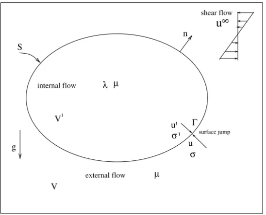
The theoretical formulation discussed in the present article will be applied to investigate densification of emulsions formed by drops of viscosityλµand radius a(undeformed shape at timet =0) immersed in a second immiscible fluid of viscosity µwith an externally imposed velocity field u∞ (see figure (1)). In the following analysis, it is assumed that the Reynolds numbers for the flows inside and outside the drop are both extremely small,Re = ρu∞a/µ, Re = ρu∞a/λµ≪ 1. It will be helpful to keep in mind thatλdenotes the viscosity ratio between the internal and the external flow, and whenλ=0 or∞the particle becomes a frictionless bubble or a rigid body, respectively.
2.1 Governing equations
In the regime of low Reynolds number, compressible fluid motions are governed by the Stokes and continuity equations
−∇
p− 1 3µ
n
u
V Γ
S
g
shear flow
u
8σ surface jump
σ
u
V
external flow µ µ
λ internal flow
Figure 1 – Sketch of the boundary conditions on a drop surface. The sketch defines the notation used in this work.
2.2 Boundary conditions
The boundary conditions on a drop interfaceSwith surface tensionŴrequire a continuous velocity across the interface and a balance between the net surface traction and surface tension forces that express the discontinuity in the interfacial surface forces [2], [11]. Mathematically, these conditions are expressed as
u→u∞ |x| → ∞; u(x)=u′(x), x=xi ∈S, (2)
whereu′denotes the flow inside the drop. For an active interface free of surface viscosity, surface elasticity and surface module of bending and dilatation, the traction jumpTTT = [[n·σ]]constitutive equation is written as [12]
TTT = [[n·σ]] =Ŵ∇s·nn−(I−nn)· ∇Ŵ. (3)
the gradient operator∇stangent to the interface,Iis the identity tensor and∇s·n denotes the mean curvature of the interfaceκ. In general, it can be expressed as the sum of the inverse principal radii of curvatureκ =(R−11+R2−1).
The force balance at the interface (3) might include both a normal traction jump(n·TTT)nand a tangential stress jump(I−nn)·TTT due to gradients of
surface tensionŴalong the interface. The dynamic effect on interfacial tension gradients are known as Marangoni effects. These variations here are associated with the presence of surfactants in the fluid. In a real flow system, we must often expectŴto vary from point to point on the interface, and it is important to consider how gradients ofŴmay influence the deformation of the drop. To describe Marangoni stress effects additional convection–diffusion equation is necessary for determining the surfactant distribution along the interface [6].
A kinematic constraint relates changes in the interface position to the local velocity. Thus interface evolution of drops are described with a Lagrangian representation
Dxi/Dt =u(xi), xi ∈S (4)
3 Integral equations
The boundary integral formulation developed in this article provides a powerful method for computing compressible Stokes flow by solving integral equations for functions that are defined over the boundaries. The important benefits of this extended approach is the ability to track deformation and swelling of drops in very dense emulsions or foam.
3.1 Reciprocal theorem for a Newtonian fluid
Consider a closed region of fluidV bounded by a surfaceS. Now consider two unrelated compressible flows of two different Newtonian fluids with densitiesρ andρ′and viscositiesµandµ′, and stress fieldsσ andσ′, respectively:
Flow 1: u,σ;(ρ, µ). The equations for conservation of mass and momentum in terms of the material derivative,D/Dt, for the flow 1 are respectively:
∇ ·u = 1 V
DV
Dt (balance of mass),
ρDu
Dt = ∇ ·
σ +ρb (balance of momentum).
(5)
Here, locally,uis the velocity, σ is the stress field andb is the external body force per unit of mass. The Newtonian constitutive equation for a compressible flow is given by Batchelor [14]
σ = −pI+2µE−2
3µ(∇ ·u)I (constitutive equation), (6)
whereIis the identity,E= 12(∇u+ ∇Tu)is the rate of strain tensor and∇Tu denotes the transpose of the tensor∇u.
Flow 2: u′,σ′;(ρ′, µ′). Similarly, the conservation and constitutive equations for the flow 2 are respectively
∇ ·u′ = 1 V′
DV′ Dt ; ρ
′Du′
Dt = ∇ ·σ
′+ρ′b′ (7)
σ′ = −p′I+2µE′−2
3µ(∇ ·u
′)I, (8)
whereE′ = 12(∇u′ + ∇Tu′) is the rate of deformation for the fluid 2. First
consider the tensorial operation
σ :E′= −pI:E′+2µE:E′−2
3µ(∇ ·u)I:E
′, (9)
but for a Newtonian compressible flow
I:E′= 1 2I :(∇u
′+ ∇Tu′)
denotes the rate of expansion of the flow [14]. Thus (9) may be written as
σ :E′ = −
p+2 3µ
′+2µE:E′ (11)
If the same steps are applied toσ′:E; it must reduce in an analogous fashion to
σ′:E= −
p′+2 3µ
′′
+2µ′E′ :E (12)
One requireE:E′=E′:Eso that
E′ :E= 1 2µ
σ :E′+
p+2 3µ
′
(13)
Now, substituting (13) into (12), ones obtain
σ′:E= −
p′+ 2 3µ
′′
+µ
′
µσ :E
′+µ′
µ
p+2 3µ
′. (14)
As a consequence of the symmetry of the stress tensorσ : ∇u′ =σT : ∇u′ = σ : ∇Tu′. Then, one may write that
σ :E′ =σ : ∇u′ = ∇ ·(u′·σ)−u′· ∇ ·σ. (15)
In this step we make the dot product of Cauchy’s equation (5) byu′ in order to define the last term in the RHS of (15). Therefore after substituting back the result of this operation into (15), it gives
σ :E′= ∇ ·(u′·σ)−ρu′·Du
Dt +ρu·b (16) By reversing the role of the primed and unprimed variables, it is also possible to obtain
σ′:E= ∇ ·(u·σ′)−ρ′u·Du
′
Dt +ρ
′u·b′ (17)
Now, substituting (16) and (17) into (14), multiplying the resultant equation byµ and make few manipulations, we obtain an expression for the generalized Lorentz reciprocal theorem for a Newtonian compressible flow (reciprocal identity):
∇ ·(µu·σ′)− ∇ ·(µ′u′·σ)
= ρ′µu·Du
′
Dt −ρµ
′u′·Du
Dt +ρµ
′(u′·b)−ρ′µ(u·b′)
+ µ′
p+ 2 3µ
′−µ
p′+2 3µ
′′
.
For low Reynolds number flow (i.e. Stokes flows) the reciprocal identity (18) takes the simpler form
∇ ·(µu·σ′)− ∇ ·(µ′u′·σ) = ρµ′(u′·b)−ρ′µ(u·b′)
+ µ′
p+2 3µ
′−µ
p′+2 3µ
′′
(19)
3.2 Integral representation for a compressible Stokes flow
Consider the particular flow of interest with velocityuand stress tensorσ. The known flow is the one due to a point force with strengthh, and located at a point xo. Suppose that the inertia of both fluids has a negligible influence on the motion of the fluid elements, and by convenience takesµ=µ′andρ =ρ′. Flow 1 and flow 2 for this particular situation are described as following.
Flow 1: u,σ. The equations for conservation of mass and momentum in terms of the material derivative,D/Dt, for the flow 1 are respectively:
∇ ·u=, ∇ ·σ = −B, (20)
whereρb = Bis the body force by unit of volume and = ∇ ·uis the flow rate of expansion.
σ = −pI+2µE−2
3µI, (21)
Flow 2: Fundamental solution of the Stokes flow; u′,σ′. The fundamental solution for Stokes equations correspond to the velocity and stress fields at a pointxproduced by a point forcehlocated atxo:
∇ ·σ′ = −B′=hδ(x−xo), ∇ ·u′=0, (22)
with| u′ |→0 and| σ′ |→ ∞as|x |→ ∞. The solution of such equations may be derived, for example, using Fourier transforms [2]
p′(x)= − h 4π · ∇
1 r
; u′(x)= 1
8π µh·G(x)ˆ ; σ
′(x)= − 3
where, the stokeslet,Gand the stressletTare defined by the following expres-sions:
G(x)ˆ = I r +
ˆ xxˆ
r3; T(x)ˆ = ˆ xxˆxˆ
r5 . (24)
The above functions are the kernels or the free-space Green’s functions that maps the forcehatxoto the fields atxin an unbounded three-dimensional domain. Herexˆ =x−xo, andr =| ˆx|. Physicallyu =G(x)ˆ ·hexpresses the velocity field due to a concentrated point forcehδ(x−xo)placed at the pointxo, and may be seen as the flow produced by the slow settling motion of a small particle.Tij k is the stress tensor associate with the Green’s functionGij andσik(x)=Tij khj is a fundamental solution of the Stokes produced by the hydrodynamic dipole D· ∇δ(x−xo). Tij k = Tkj i as required by symmetry of the stress tensorσ. It is straightforward to show that the Reciprocal theorem for the present case, equation (19), takes the form
∇ ·(u·σ′)− ∇ ·(u′·σ)=u′·B−u·B′−p′ (25)
Now, considering the body force exerted on the flow(u,σ)the gravity force B= ∇(ρg·x), substituting the expressions of the point-force solution into (25) and discarding the arbitrary constanthones obtain
− 3
4π∇ · [u(x)·T(x)ˆ ] − 1
8π µ∇ · [G(x)ˆ ·σ(x)]
= 8π µ1 [G(x)(ρgˆ ·x)] +u(x)δ(x)ˆ + 1 4π∇
1 r
.
(26)
Note that we have used for the first term on the RHS of equation (26), the incompressibility of the singular solution∇ ·G = 0, so thatG· ∇(ρg·x) = ∇ · [G(ρg·x)]. The above equation is valid everywhere except at the singular pointxo.
S
n
n
n
xo
xo V
Vε
ε
V V
S
(a)
(b)
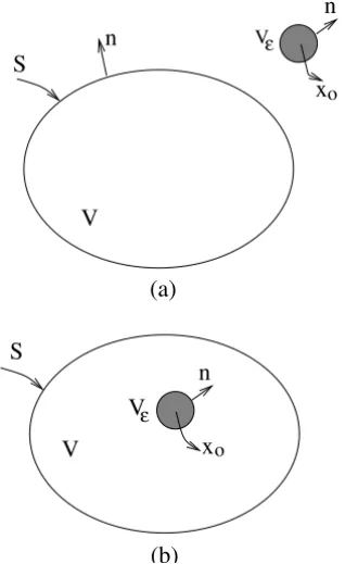
Figure 2 – Schematic sketch for the integration domain with singularity outside (a) and inside volumeV (b).
Point force outsideV. For this caseδ(x−xo) = 0 insideV and thus after integrating equation (26) the integral representation of the Reciprocal theorem takes the form
−4π3
V∇ · [
u(x)·T(x)ˆ ]dV − 1 8π µ
V∇ · [
G(x)ˆ ·σ(x)]dV
= 8π µ1
V∇ · [
G(x)(ρˆ g·x)]dV + 4π
V ∇
(r−1) dV
(27)
The volume integrals in equation (27) can be converted to the surface integrals overS, by using the divergence theorem obtaining
1 8π µ
S
G(x)ˆ ·σ(x)·n(x) dSx+ 3 4π
S
u(x)·T(x)ˆ ·n(x) dSx
+ 1 8π µ
S
G(x)(ρgˆ ·x)·n(x) dSx+ 4π
S
r−1n(x) dSx =0,
wherenis the unit outward normal to the surfaceS. Equation (28) is the integral representation of the flow if the singularity is outsideV. It will be shown that the integral equation (28) is a useful identity for developing new integral equations in terms of jump conditions on the interface.
Point force insideV. In order to formally determine the integral representation for the situation which δ(x−xo) = 0 insideV, we must integrate again the equation (26). Applying the divergence theorem andδ-distribution property, one obtains
u(xo)= − 1 8π µ
S
G(x)ˆ ·σ(x)·n(x) dSx
−4π3
S
u(x)·T(x)ˆ ·n(x) dSx− 1 8π µ
S
G(x)(ρgˆ ·x)·n(x) dSx
−4π
S
r−1n(x) dSx,
(29)
Equation (29) is the integral representation for compressible Stokes in terms of four boundary distributions involving the Greens’s functionsG, the stresslet T and the potential source 1/r. The first distribution on the RHS of (29) is termed the single-layer potential, the second distribution is termed double layer potential, whereas the last new term is a potential source distribution due to the compressibility of the flow with a constant rate of expansion.
3.3 Integral representation in terms of the traction jump
External flow representation. Using the reciprocal identity (28) for the inter-nal flowu′(inside the particle) at a pointxothat is located exterior to the particle, one obtain
1 8π µ
S
G(x)ˆ ·σ′(x)·n(x) dSx+ 3λ 4π
S
u′(x)·T(x)ˆ ·n(x) dSx
+ 8π µ1
S
G(x)(ρˆ ′g·x)·n(x) dSx+λ
′
4π
S
r−1n(x) dSx =0,
(30)
obtained as a function of the traction jumpTTT,
u(xo) = u∞(xo)− 1 8π µ
S
G(x)ˆ ·T(x) dSx
−4π3
S[
u(x)−λu′(x)] ·T(x)ˆ ·n(x) dSx
−8π µ1
S
G(x)(ρgˆ ·x)·n(x) dSx− −λ
′
4π
S
r−1n(x) dSx, (31)
Internal flow representation. We repeat the above procedure for the internal flow. Hence, the integral representation of the internal flow is obtained when equation (29) is applied,
u′(xo) = 1 8π λµ
S
G(x)ˆ ·σ′(x)·n(x) dSx
+ 3λ 4π
S
u′(x)·T(x)ˆ ·n(x) dSx
+ 8π λµ1
S
G(x)(ρˆ ′g·x)·n(x) dSx+
′
4π
S
r−1n(x) dSx,
(32)
Using the reciprocal identity (26) for the external flowu′(outside the particle) at a pointxothat is located in the interior of the particle, one obtain after dividing the full equation byλ, that
u∞(xo)
λ −
1 8π λµ
S
G(x)ˆ ·σ(x)·n(x) dSx
− 3
4π λ
S
u(x)·T(x)ˆ ·n(x) dSx
− 8π λµ1
S
G(x)(ρgˆ ·x)·n(x) dSx− 4π λ
S
r−1n(x) dSx =0. (33)
The integral representation of the internal flow as a function of the jump con-dition is obtained by combining (32) and (33)
λu′(xo) = u∞(xo)− 1 8π µ
S
G(x)ˆ ·T(x) dSx
− 3 4π
S[
u(x)−λu′(x)] ·T(x)ˆ ·n(x) dSx
− 1
8π µ
S
G(x)(ρˆ ′g·x)·n(x) dSx−−λ
′
4π
S
3.3.1 Integral representation for the interface.
The integral representation for the flow solution at the interface is found by applying the jump condition(1/2)[u(xo)+λu′(xo)] to the equations (31) and (34) (see figure 1). For the limit ofxo going to the interface, u(xo) = u′(xo) (continuity of velocity) and the traction discontinuityTTTis given by the equation
(3). Under these conditions only the integral representation for the fluid-fluid interfaceSneed to be considered, hence
(1+λ)u(xo) = 2u∞(xo)−A
S
G(x)ˆ ·TTT(x) dSx
+B
S
u(x)·T(x)ˆ ·n(x) dSx−A
S
G(x)(ρˆ g·x)·n(x) dSx
+(λ′−) 2π
S
r−1n(x) dSx,
(35)
where A = 1/4π µand B = 2π3 (λ−1). It should be noted that when the viscosity ratio λ = 1.0 and ρ = 0 the double layer and the single layer integrals (related to the buoyancy force) vanish and the flow is expressed merely in terms of a single-layer potential with known density forceTTT and the source
potential integral. This means that the same fluid is occupying all space, but with a membrane of points force and sources provide by the singularities at the positions of the interface.
4 Application
4.1 Interacting drops
All simulations rely on the boundary integral method. Periodic boundary con-ditions are enforced through the use of periodic Greens functions. These are obtained by Ewald summation [16] using accurate computationally-efficient tab-ulation of the nonsingular background contribution [7]. The appropriate formu-lation was derived in §3. The resulting boundary integral formuformu-lation are now capable of describing the dynamics of dense emulsions for uniform compress-ibility. Accordingly, the evolution of M neutrally buoyant deformable drops is described by time-integrating the fluid velocityu(xo) on a set of interfacial marker pointsx0on each drop surface. In the present application it is considered the case in which there is a rapid equilibrium of insoluble surfactants (incom-pressible surfactants). Therefore, Marangoni stresses and adsorption–desorption of surfactants can be ignored.
All quantities below are made dimensionless using the (volume–averaged) drop size a and the relaxation rate Ŵ/µa. The relevant physical parameters that describe the simulated system simulated are: λ,φ and the compressibility parameter,Cao = aµ/ Ŵ(ratio of viscous to surface tension stress). Caois the appropriate capillary number for the densification process. In the absence of an imposed flow (i.e.u∞(xo)=0), the dimensionless fluid velocity is governed by the second-kind integral equation on the interfacesSm (m =1,· · ·, M) of all simulated drops.
(1+λ)u(xo)−B M
m=1
Sm
u(x)·TP(x)ˆ ·n(x) dSx =F(x), (36)
where
F(x) = − 1 4π
M
m=1
Sm
Ŵ(∇s ·n)GP(x)ˆ ·n(x) dSx
+ Caof (φ)π M
m=1
Sm
P(r)n(x) dSx.
(37)
GP and TP are respectively the periodic stokeslet and stresslet defined as in reference [17], P is the periodically-replicated r−1 potential and f (φ) = −
The volume-averaged stress tensor from the dispersed phase is obtained from an integral of the traction jump and fluid velocity over the drop interfaces [14],
= 1 M
M
m=1
Sm
(∇s·n)xn+µ(λ−1)(un+nu)
dS(x). (38)
Equation (38) is the contribution of the dispersed phase to the macroscopic stress of the emulsion due to the dipole stresslet that each drop torque free generates in the flow. The (volume-averaged) non-equilibrium osmotic pressure during densification ist r ()−2φ, where tr() is the trace of the stress tensor, and 2φis the contribution from the capillary pressure of spherical drops. When densification stops, the drop shapes relax, and the stress relaxes to the equilibrium osmotic pressure which depends only on the drop shapes.
4.2 Numerical results
Runge-Kutta scheme. An appropriate time step that is proportional to the shortest edge length is set in order to ensure stability.
The adaptive surface triangulation algorithm, described in [10], has been ex-tended to construct efficient simulations of dense systems. Accordingly, a new marker point density function was defined that resolves the minimum local length scale everywhere on the drop interfaces. For the proposed problem the minimum local length scale may depend on the local curvature or local film thicknessh. Thus, the marker point density function [10] should be generalized to:
ρN ∼
R1−2+R−22+C1
|∇sh| h
2
, (39)
whereR1, R2are the local principal radii of curvature, andC1areO(1)constants whose precise value is unimportant. The proposed marker point density function (39) resolves the rim of dimpled regions where the film thickness varies rapidly and the lubrication length scale √hR in regions where the film thickness is slowly-varying (R =min[R1, R2]). Only rim regions, not flat regions, require high resolution.
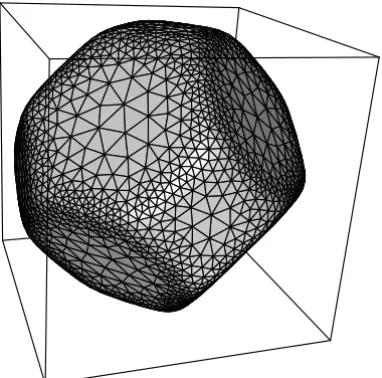
An inspection of the result in figure 3, which was obtained using the density
function (39), illustrates this point: high resolution is needed on the plateau borders and junctions, not on the flat films between drops. This observation is important for ensuring the feasibility of accurately resolving the dynamics of the closely-spaced interfaces that characterize the dense systems that we have explored.
The surface integrations in Equations (36), involve singular integrand. Trapezoid-rule integration with singularity subtraction and near-singularity sub-traction for closely-spaced interfaces of drops (if surface tension gradients are not present) [7] can be used to accurately evaluate the integrals. Equation (36) has eigensolutions that cause unphysical changes in the dispersed-phase volume at small viscosity ratios, corrupt numerical solutions at large viscosity ratios, and slow the iterative convergence. These effects were eliminated by imple-menting Wielandt eigenvalue deflation described in [2] in order to purge the solutions corresponding toλ=0 andλ= ∞. The resulting surface integration algorithm is economical andO(1/N )accurate, consistent with the triangulated representation of the drop interface.
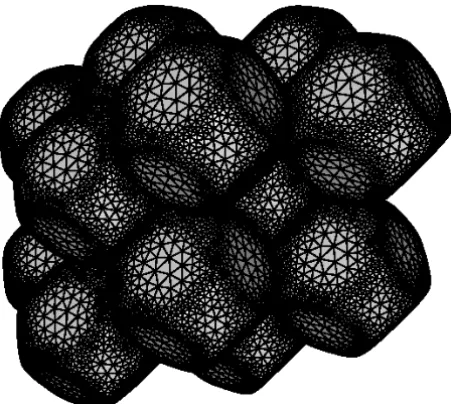
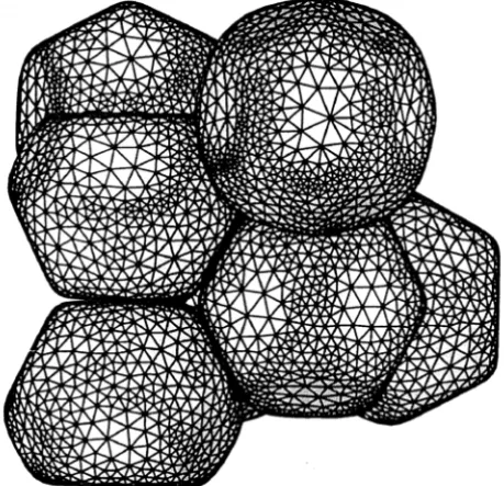
Figure 4 – Simulation result for a Kelvin microstructure of a dense emulsion resulting from expansion of the dispersed-phase withCao =0.5,φ=0.95 andλ=1.0 (BCC
A wide range of densification processes can be simulated through the appropri-ateφdependence (i.e., time-dependence) of. It is also possible to explore mi-crostructural manipulation through an applied shear during densification. Here, we consider constant compressibility, quiescent flow conditions and the case λ = 1.0 because the numerical implementation is simpler. Densification with prescribed non-equilibrium osmotic pressure has been also explored since it cor-responds most closely to the experimental procedure that has been developed [15]. Under these conditions, densification proceeds until the applied osmotic pressure is balanced by the equilibrium osmotic pressure of the emulsion. The Kelvin-cell and Weaire-Phelan microstructure, depicted in figures (6) and (5), were obtained using an algorithm based on the compressible formulation dis-cussed in §3.
Figure 5 – Microstructure of a dense emulsion resulting from expansion of the dis-persed-phase withα=0.5 (rate of expansion),φ=0.95 andλ=1.0. Weaire-Phelan foam (with eight particle per cell).
Spherical drops on a BBC lattice make first contact with eight nearest neighbors and form precursors of hexagonal faces whenφ < φc =π31/2/8
70% 80%
95%
98% 90%
Figure 6 – Kelvin-cell emulsion resulting from expansion of the dispersed-phase with
Cao=0.5 followed by 20 time units of drop relaxation; dispersed-phase volume fraction
up to 98% as labeled;λ=1.0.
the evolution of drop shape from spheres to Kelvin cells. Once the emulsion expansion has stopped, the drop shape will continue to relax toward equilibrium. This process is illustrated in figure (6); the emulsion expand and then relaxes for twenty time units. We have no experimental results with which compare our numerical predictions.
5 Conclusion
made substantial progress on the problem of emulsion densification. The results demonstrate the feasibility of simulating high-volume-fraction systems. A study of densification may have interesting materials processing applications that will be pursued in a future study.
6 Acknowledgment
The authors are grateful to the CAPES-Brazil, CNPq-Brazil and CT-Petro-Finep for their generous support of this work. We would like to thanks Dr. Vittorio Cristini and Dr. Jerzy Blawzdziewicz for helpful discussions on their algorithm for adaptive mesh restructuring of three-dimensional drop surface.
REFERENCES
[1] G.K. Youngren and A. Acrivos,Stokes flow past a particle of arbitrary shape: A numerical method of solution, J. Fluid Mech.,69(1975), pp. 377–403.
[2] C. Pozrikidis,Boundary integral and singularity methods for linearized viscous flow, Cam-bridge University Press, CamCam-bridge, (1992).
[3] O.A. Ladyzheskaya,The mathematical theory of viscous incompressible flow, Gordon & Breach, New York, (1969).
[4] J.M. Rallison and A. Acrivos,A numerical study of the deformation and burst of a viscous drop in an extensional flow, J. Fluid Mech.,89(1978), pp. 191–200.
[5] J.M. Rallison,The deformation of small viscous drops and bubbles in shear flows, Ann. Rev. Fluid Mech.,16(1984), pp. 45–66.
[6] H.A. Stone,Dynamics of drop deformation and breakup in viscous fluids, Ann. Rev. Fluid Mech.,26(1994), pp. 65–102.
[7] M. Loewenberg and E.J. Hinch,Numerical simulations of a concentrated emulsion in shear flow, J. Fluid Mech.,321(1996), pp. 395-419.
[8] F.R. Cunha, M. Neimer, J. Blawzdziewicz and M. Loewenberg,Rheology of an Emulsion in Shear Flow, In: Proceedings of American Institute of Chemical Engineers, Annual Meeting, Fundamental Research in Fluid Mechanics: Particulate & Multiphase Flow II., paper 124j., October (1999).
[9] F.R. Cunha and M. Loewenberg,Emulsion Drops in Oscillatory Shear FlowIn: 52nd American Physical Society, Annual Meeting of the Division of Fluid Dynamics, paper GK. 08, session: suspension I, November (1999).
[11] G.L. Leal, Laminar flow and convective transport processes, Butterworth-Heinemann, Boston, (1992).
[12] L.E. Scriven,Dynamics of fluid interface, Chem. Eng. Science,12(1960), pp. 98-108.
[13] J. Happel and H. Brenner,Low Reynolds number hydrodynamics, Prentice Hall, (1965).
[14] G.K. Batchelor,An introduction to Fluid Dynamics, Cambridge University Press, Cambridge, (1967).
[15]T.G. Mason, M.D. Lacasse, S.G. Grest, D. Levine, J. Bibette and D.A. Weitz,Osmotic pressure and viscoelasticity shear moduli of concentrated emulsions, Physical Review E,56(1997), pp. 3150.
[16] C.W.J. Beenakker, Ewald sum of Rotne-Prager tensor, J. Chem. Phys.,85 (1986), pp. 1581–1582.
[17] M.P. Almeida and F.R. Cunha,Numerical simulation of non-colloidal deformable particles at low Reynolds numbers, In: Proceedings, 7th Brazilian Congress of Engineering and Thermal Sciences,1(1998), pp. 963–970.