ISSN 0104-6632 Printed in Brazil
www.abeq.org.br/bjche
Vol. 29, No. 02, pp. 359 - 369, April - June, 2012
*To whom correspondence should be addressed
Brazilian Journal
of Chemical
Engineering
MODELLING OF FERTILIZER DRYING IN A
ROTARY DRYER: PARAMETRIC SENSITIVITY
ANALYSIS
M. G. Silva
1, T. S. Lira
2, E. B. Arruda
3, V. V. Murata
1and M. A. S. Barrozo
1*1
School of Chemical Engineering, Federal University of Uberlândia, Phone: + (55) (34) 32394292, Fax: + (55) (34) 32394188, Av. João Naves de Ávila 2121, Uberlândia - MG, Brazil.
E-mail: masbarrozo@pesquisador.cnpq.br
2
Departament of Engineering and Computation, Federal University of Espírito Santo, Rod. BR 101 Norte, km. 60, São Mateus - ES, Brazil.
3
School of Integrated Sciences of Pontal, Federal University of Uberlândia, Av. José João Dib 2545, Ituiutaba - MG, Brazil.
(Submitted: August 22, 2011 ; Revised: September 18, 2011 ; Accepted: December 22, 2011)
Abstract - This study analyzed the influence of the following parameters: overall volumetric heat transfer coefficient, coefficient of heat loss, drying rate, specific heat of the solid and specific heat of dry air on the prediction of a model for the fertilizer drying in rotary dryers. The method of parametric sensitivity using an experimental design was employed in this study. All parameters studied significantly affected the responses of the drying model. In general, the model showed greater sensitivity to the parameters drying rate and overall volumetric heat transfer coefficient.
Keywords: Heat and mass transfer; Fertilizer drying; Rotary dryers; Parametric sensitivity.
INTRODUCTION
Rotary dryers are often used for drying in fertilizer industries. They consist basically of a long cylindrical shell inclined at a small angle to the horizontal. The inside portion of the shell is equipped with lifting flights (see Figure 1) to cascade solid material through a concurrent or counter-current gas stream (Sheehan et al., 2005). Wet feed is introduced into the upper end of the dryer and the dried product withdrawn at the lower end.
The performance of rotary dryers is dictated by three important transport phenomena, namely: solids
transportation (Lisboa et al., 2007, Cao and
Langrish, 1999; Renaud et al., 2000; Shahhosseini et al., 2000; Song et al., 2003; Britton et al., 2006), heat, and mass transfer (Arruda et al., 2009a; Lobato et al., 2008). The ability to estimate each of these transport mechanisms is essential for proper design and operation of rotary dryers (Krokida et al., 2002).
The movement of particles in rotating drums depends on the flights and shell design, as well as on the operating conditions. Thus, rotary dryers represent one of the greatest challenges in theoretical modelling of dryers (Sherrit et al., 1993). The complex combination of particles being lifted by the flights, sliding and rolling, then falling in spreading cascades through an air stream and re-entering the bed at the bottom, possibly with bouncing and rolling, is very difficult to analyze (Kemp, 2004).
Feed Shell
Flights
Rotation System
Discharge Figure 1: The conventional rotary cascade dryer.
Arruda (2008) developed a general model for the drying process in a conventional rotary dryer that could be applied to any type of particulate material. This author found good agreement of the simulated results from this model with experimental data for fertilizer drying. However, Fernandes et al. (2009) comment that the deviations of this model simulation from their experimental data for an industrial dryer could be explained by the imprecision of the parameters of the constitutive equations. Actually, the model proposed by Arruda (2008) is quite general and the parameters of the constitutive equations were obtained from specific studies, such as a thin layer dryer for the drying kinetics equation and a static method for equilibrium moisture content. Thus, this approach had no adjustable parameters, allowing a realistic analysis of the prediction from the model. Therefore, is very important to analyze the sensitivity of the responses of the model to the variation of the parameters in the main constitutive equations to identify possible weaknesses in the model prediction and thus improve the model. Thus, the purpose of this work was to analyze the influence of the following parameters: overall volumetric heat transfer coefficient, coefficient of heat loss, drying rate, specific heat of the solid and specific heat of dry air on the prediction model proposed by Arruda (2008). The method of parametric sensitivity using experimental design was employed in this study. The results of the simulation are compared with experimental data for
granulated single superphosphate (SSPG) obtained from a rotary dryer in a pilot scale unit.
MATHEMATICAL MODELLING
Simultaneous Transfer of Mass and Energy in Rotary Dryers
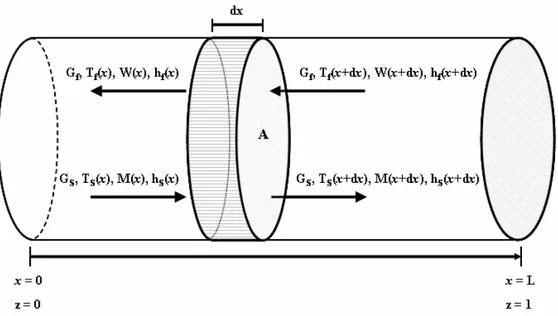
Modelling of the drying process in moving bed dryers is based on applying the equations of conservation of mass and energy to the fluid and particulate phases in infinitesimal volume elements of the dryer (Barrozo et al., 2001). Figure 2 shows the scheme of the infinitesimal volume element of a conventional rotary dryer operating in countercurrent flow (Arruda, 2008). The modelling approach considers the fluid dynamic characteristics of the dryer, as well as the intrinsic properties of the material, equilibrium moisture and drying kinetics.
In the formulation of this model, the following assumptions were made:
The particle axial velocity through the drum is constant (vs =L τ);
The drying rate is evaluated in each infinitesimal volume element volume of the dryer;
Grain shape and physicochemical properties of
solid and fluid phases (Cps, Cpl, Cpv, Cpf and λ) do
not change during drying;
The initial conditions of solid feeding flow,
Brazilian Journal of Chemical Engineering Vol. 29, No. 02, pp. 359 - 369, April - June, 2012
Figure 2: Schematic of the infinitesimal volume element of the rotary dryer operating at countercurrent flow.
The equation system from the balances of mass and energy between drying gas and particulate material is presented next, where z is the dimensionless length, given by the proportion between a given position (x) and the total length of the dryer (L).
* w
f
dW R H
=-dz G (1)
* w
S
dM R H
=-dz G (2)
*
va f S w v f P f amb
f
f f v
U V(T -T )+R H (λ+Cp T )
+U πDL(T -T )
dT =
dz G (Cp +WCp )
⎡ ⎤
⎢ ⎥
⎣ ⎦ (3)
* va f S w l S
w v f S
S
S S l
U V(T -T )+R H Cp T + -R H[λ+Cp (T -T )] dT
=
dz G (Cp +MCp )
⎡ ⎤
⎢ ⎥
⎣ ⎦ (4)
The system of differential equations of the model should be resolved simultaneously for the four variables involved, considering the contour
conditions that follow: W(L)=W ; 0 M(0)=M ; 0
f f0
T (L)=T ; T (0)=T . S S0
Drying in conventional cascading rotary dryers occurs mostly during the time in which the particles are falling from the flights, when they are in contact
with the dry air, which corresponds to only a fraction of the residence time (Baker, 1983). As proposed by Arruda (2008), this fraction refers to the effective contact time between the solid and dry air (ftef) and can be evaluated by the relation
between the average falling time of the particle and total time of a cycle. This, in turn, corresponds to the time spent from material collection by the flight until its return to the particle bed on the bottom of the drum. This fraction can be evaluated by Equation (5), where the total number of cycles (NCi)
is given by Equation (6) and the effective contact time between the gas and the particles (tef), by
Equation (7). The total solids load in the dryer (H*) is given by Equation (8).
q Ci Ci q tef
Ci Ci
t N N t
f = × =
N
t τ (5)
Ci
q
L L
N = =
l Y sin(α) (6)
ef tef
t =f ×τ (7)
* S
H =τ×G (8)
For the conventional rotary dyer, the effective contact time between the gas and the particles (tef)
Constitutive Equations
Equilibrium Moisture
Based on experimental data of equilibrium moisture content of simple superphosphate fertilizer, Arruda (2008) performed a statistical study of discriminating rival models and concluded that the modified Halsey correlation (Ribeiro et al., 2005) best adjusted his experimental data. The modified Halsey equation with the parameters estimated by Arruda (2008) for superphosphate fertilizer is presented next.
(
)
( )
1 1.435 S
eq
-exp -0.045T -2.08 M =
ln RH
⎛ ⎞
⎜ ⎟
⎝ ⎠ (9)
Drying Kinetics
Arruda (2008) performed an experimental study in a thin layer dryer (Barrozo et al., 2006), and concluded that the best correlation to represent the drying kinetics of the fertilizer was Page’s equation (1949). This equation, with the parameters estimated by Arruda (2008) for simple superphosphate, is presented subsequently:
eq
0 eq
0.392
f M-M
MR= =
M -M
-121.845
exp -0.431exp ( z)
T
⎡ ⎛ ⎞ ⎤
τ
⎢ ⎜ ⎟ ⎥
⎝ ⎠
⎣ ⎦
(10)
where zτ is equivalent to the time of drying.
Thus, the drying rate can be calculated by Equation (11).
(
)
(
0 eq)
wMR-1 M -M -R =
( z)τ (11)
Heat Transfer Coefficients
The best correlations for the overall volumetric heat transfer coefficient (Uva) and for the heat lost
through the wall coefficient (UP) were also
determined by Arruda (2008). These equations with the parameters estimated in this previous work are:
0.289 0.541
va f s
U =0.394g g (12)
0.879
P f
U =0.022g (13)
SENSITIVITY ANALYSIS USING EXPERIMENTAL DESIGN
The values of the parameters for the simulations in this sensitivity analysis study were established using an orthogonal central composite design (Box et al., 1978), which involved a total of 46 simulations for each operating condition shown in Table 1.
Table 1: Values of the operating conditions (α = 3º; NR = 3.6 rpm; Gf = 0.15 kg min1).
Conditions Variable
1 2 3
vf (m s-1) 1.5 2.5 3.5
Tf (oC) 75 85 95
Gs (kg min-1) 1.2 1.0 0.8
The parameters studied here were: drying rate (Rw), overall volumetric heat transfer coefficient (Uva),
coefficient of heat loss (Up), specific heat of the solid
(Cps) and specific heat of dry air (Cpf). Solid moisture
content (M) and solid temperature (Ts) were used as
response variables. Equations (14) to (18) present the dimensionless form of these parameters and Table 2 shows the levels of the parameters applied in this work. Rw, Uva and Up at different levels in Table 2
were obtained by multiplying Equations (11) to (13), respectively, by a factor.
Table 2: Levels of the parameters.
Levels Parameters
-α -1 0 +1 +α
Rw (min-1) 0.90*Eq.(11) 0.94*Eq.(11) 1.00*Eq.(11) 1.06*Eq.(11) 1.10*Eq.(11)
Uva (kW m-3 oC-1) 0.90*Eq.(12) 0.94*Eq.(12) 1.00*Eq.(12) 1.06*Eq.(12) 1.10*Eq.(12)
Up (kW m-2 oC-1) 0.90*Eq.(13) 0.94*Eq.(13) 1.00*Eq.(13) 1.06*Eq.(13) 1.10*Eq.(13)
Cps (kJ kg-1 °C-1) 0.923 0.968 1.026 1.083 1.128
Brazilian Journal of Chemical Engineering Vol. 29, No. 02, pp. 359 - 369, April - June, 2012
[
va va]
1
va va U -U (0) x =
U (1)-U (-1) /2 (14)
[
P P]
2
P P
U -U (0) x =
U (1)-U (-1) /2 (15)
[
w w]
3
w w
R -R (0) x =
R (1)-R (-1) /2 (16)
s 4
Cp -1.026 x =
0.057 (17)
f 5
Cp -1.000 x =
0.056 (18)
where x1, x2, x3, x4 and x5 are the dimensionless
forms of the Rw, Uva, Up, Cps, and Cpf parameters,
respectively.
The levels -1 and +1 of each parameter were chosen so that the difference between the extreme values of the interval (-α and α) and the central level did not exceed 10% of the parameter’s original value. The value of α (extreme dimensionless level) of the experimental design was 1.784. This value leads to an orthogonal central composite design, i.e., a design in which the variance and covariance matrices are diagonals, and the parameters are uncorrelated.
RESULTS AND DISCUSSION
Figure 3 show the results of the comparisons between experimental data (Arruda 2008) for the solids moisture content, obtained at the end of the dryer (z=1), and those computed by the model with the parameters in the central levels of Table 2. The experimental data were obtained by Arruda (2008) with a conventional rotary dryer equipped with three-segmented angular flights. The flights had the dimensions: first segment = 0.02 m, second and third segment = 0.007 m; the length of the flights was 1.5 m,
with an angle of 135o between segments. The
operating conditions of the experiments performed by Arruda (2008) are presented in Table 3.
A good agreement between the simulated values of solids moisture content and those obtained experimentally in the rotary cascading dryer can be observed in the results presented in Figure 3. The average deviation of the simulation results in relation to the experimental data was 7.7 %. These deviations
were probably caused by measurement imprecision and/or inaccuracy of the model parameters.
Table 3: Experimental design (Arruda, 2008).
Experiment vf (m/s)
(m/s)
Tf (oC)
(oC)
Gs (kg/min)
(kg/min)
1 1.5 75 0.8
2 1.5 75 1.2
3 1.5 95 0.8
4 1.5 95 1.2
5 3.5 75 0.8
6 3.5 75 1.2
7 3.5 95 0.8
8 3.5 95 1.2
9 1.09 85 1
10 3.91 85 1
11 2.5 70.9 1
12 2.5 99.1 1
13 2.5 85 0.72
14 2.5 85 1.28
15 2.5 85 1
Experiment M ( k gwa te r /k gdr y s o li d )
0 1 2 3 4 5 6 7 8 9 10 11 12 13 14 15 16 0.00 0.02 0.04 0.06 0.08 0.10 0.12 0.14 0.16 0.18 0.20
Experimental (z=1) Predict (z=1)
Figure 3: Experimental and simulated results for the solids moisture content at the exit of the conventional dryer for each experiment (see conditions in Table 3).
The resolution of the differential equation system (Equations (1) to (4)) was obtained by the technique of normal collocation with 10 placement points for the 4th order polynomial approximation, using the
sub-routine “bvp4c” of MATLAB® software. The
relative tolerance used was 10-6. The simulated results (values of response variables at the end of the countercurrent rotary dryer, i.e., for the solid at z = 1)
were analyzed statistically using STATISTICA®
software, with each of the responses subjected to an analysis of variance. The parameters whose level of significance exceeded 5% were neglected (in a hypothesis test using Student’s distribution) and the respective parameters were considered irrelevant.
Equations (19) and (20) represent the matrix forms of the equations fitted for the solid moisture content
respectively, as functions of the dimensionless parameters (overall volumetric heat transfer coefficient: x1; coefficient of heat loss: x2; drying
rate: x3; specific heat of solid: x4; and specific heat
of dry air: x5). In the equations, the interactions and
quadratic effects (r = 0.999) are present, beyond the main effects. It was observed that the highest values of the coefficients of the main effects in Equations (19) and (20) were for the parameters drying rate (x3) and overall volumetric heat transfer coefficient
(x1). These results demonstrate that both Uva and Rw
are the most important parameters to be considered in the model. Moreover, all coefficients were retained in Equation (19), because all parameters were significant for the solid moisture content, i.e., the levels of significance did not exceed 5% as shown in Table 4. In Equation (20), the coefficients of the quadratic term (x22) and interaction terms
(x2x4 and x4x5) were equal to zero because these
coefficients were irrelevant for the solid temperature, i.e., the levels of significance exceeded 5% (see Table 5).
M=0.1237+x ' b+x ' Bx (19)
where: 1 2 3 4 5 x x x x x x ⎡ ⎤ ⎢ ⎥ ⎢ ⎥ = ⎢ ⎥ ⎢ ⎥ ⎢ ⎥ ⎢ ⎥ ⎣ ⎦ ; -0.000200 0.000109 b -0.000644 0.000100 -0.000191 ⎡ ⎤ ⎢+ ⎥ ⎢ ⎥ = ⎢ ⎥ ⎢+ ⎥ ⎢ ⎥ ⎢ ⎥ ⎣ ⎦ and
0.000007 0.000001 -0.000006 0.0000005 -0.00000025
0.000001 -0.000001 0.0000025 -0.0000005 -0.000002
B -0.000006 0.0000025 0.000007 0.0000015 -0.0000055
0.0000005 -0.0000005 0.0000015 -0.00
-0.00000025 -0.000002
+ + +
+ +
= + + +
+ + 0002 0.0000005
-0.0000055 0.0000005 0.000009
⎡ ⎤ ⎢ ⎥ ⎢ ⎥ ⎢ ⎥ ⎢ ⎥ ⎢ ⎥ ⎢ ⎥ ⎢ ⎥ ⎢ ⎥ ⎢ ⎥⎦ ⎣ + + + s
T =47.72+x ' b+x ' Bx (20)
where: 1 2 3 4 5 x x x x x x ⎡ ⎤ ⎢ ⎥ ⎢ ⎥ = ⎢ ⎥ ⎢ ⎥ ⎢ ⎥ ⎢ ⎥ ⎣ ⎦ ; 1.16796 -0.11462 b -0.69211 -0.36060 0.20112 + ⎡ ⎤ ⎢ ⎥ ⎢ ⎥ = ⎢ ⎥ ⎢ ⎥ ⎢ ⎥ + ⎢ ⎥ ⎣ ⎦ and
-0.02749 -0.00233 -0.00063 -0.00478 0.005125
-0.00233 0.00000 0.002335 0.00000 0.002275
B -0.00063 0.002335 0.00611 0.009325 -0.002925
-0.00478 0.00000 0.009325 0.00360 0.00000
0.005125 0.002275 -0.002925
+ ⎡ ⎢ + + ⎢ = ⎢ + + + ⎢ + + ⎢ ⎢+ +
⎣ 0.00000 -0.00965
Brazilian Journal of Chemical Engineering Vol. 29, No. 02, pp. 359 - 369, April - June, 2012
Table 4: Regression coefficients and statistical tests for the solid moisture content (M).
Factor Regression
Coeff. Std. Err. t(25) p Mean/Interc. 0.123719 0.000001 244684.0 <10-6
x1 -0.000200 <10-6 -1075.0 <10-6
x12 0.000007 <10-6 26.5 <10-6
x2 0.000109 <10-6 585.5 <10-6
x22 -0.000001 <10-6 -2.2 0.035841
x3 -0.000644 <10-6 -3471.1 <10-6
x32 0.000007 <10-6 25.8 <10-6
x4 0.000100 <10-6 537.4 <10-6
x42 -0.000002 <10-6 -6.0 0.000003
x5 -0.000191 <10-6 -1027.0 <10-6
x52 0.000009 <10-6 35.3 <10-6
x1x2 0.000002 <10-6 9.1 <10-6
x1x3 -0.000012 <10-6 -59.7 <10-6
x1x4 0.000001 <10-6 6.5 0.000001
x1x5 -0.000005 <10-6 -25.9 <10-6
x2x3 0.000005 <10-6 23.5 <10-6
x2x4 -0.000001 <10-6 -4.2 0.000280
x2x5 -0.000004 <10-6 -20.5 <10-6
x3x4 0.000003 <10-6 15.0 <10-6
x3x5 -0.000011 <10-6 -51.8 <10-6
x4x5 0.000001 <10-6 5.8 0.000005
Table 5: Regression coefficients and statistical tests for the solid temperature (Ts).
Factor Regression
Coeff. Std. Err. t(25) p Mean/Interc. 47.71602 0.000751 63499.97 <10-6
x1 1.16796 0.000276 4233.50 <10-6
x12 -0.02749 0.000380 -72.41 <10-6
x2 -0.11462 0.000276 -415.45 <10-6
x22 0.00057 0.000380 1.49 0.147741
x3 -0.69211 0.000276 -2508.67 <10-6
x32 0.00611 0.000380 16.10 <10-6
x4 -0.36060 0.000276 -1307.07 <10-6
x42 0.00360 0.000380 9.48 <10-6
x5 0.20112 0.000276 729.01 <10-6
x52 -0.00965 0.000380 -25.41 <10-6
x1x2 -0.00466 0.000302 -15.42 <10-6
x1x3 -0.00126 0.000302 -4.18 0.000315
x1x4 -0.00956 0.000302 -31.66 <10-6
x1x5 0.01025 0.000302 33.95 <10-6
x2x3 0.00467 0.000302 15.45 <10-6
x2x4 0.00048 0.000302 1.59 0.123429
x2x5 0.00455 0.000302 15.05 <10-6
x3x4 0.01865 0.000302 61.73 <10-6
x3x5 -0.00585 0.000302 -19.36 <10-6
x4x5 -0.00050 0.000302 -1.65 0.111414
Response surfaces were generated from Equations (19) and (20) for the solid moisture
content (M) and the solid temperature (Ts) as
functions of the most important parameters (Figures
4 and 5, respectively). Even though most of the quadratic and interaction coefficients are significant, the response surfaces look rather flat, because the quadratic and interaction coefficients are orders of magnitude smaller than the linear coefficients.
Figure 4: Response surface of solid moisture content (M) as a function of the drying rate (Rw or x3) and the
overall volumetric heat transfer coefficient (Uva or x1)
for condition 2.
Figure 5: Response surface of solid temperature (Ts)
as a function of the drying rate (Rw or x3) and the
overall volumetric heat transfer coefficient (Uva or x1) for
condition 2.
As expected, the lowest values of solid moisture content (M) were achieved for the highest values of drying rate (Rw or x3) and overall volumetric heat
transfer coefficient (Uva or x1). Lower values of solid
temperature (Ts) were achieved for higher values of
Additional simulations with perturbations of ± 20% in the values of the parameters (Uva, Up, Rw, Cps, Cpf)
were performed. The impact (in percentage) of the perturbations (± 10% and ± 20%) in solid temperature (Ts) at the end of the dryer are shown in Table 6 for the
three operating conditions presented in Table 1. In general, it is observed that the variations of solid temperature (Ts) were up to -10.5%, i. e., values
greater than the experimental uncertainty. Again, the parameters that affected the solid temperature (Ts) the
most were the drying rate (Rw) and the overall
volumetric heat transfer coefficient (Uva).
Figures 6 and 7 show the solid moisture content
(M) profiles as a function of the dimensionless length of the dryer (z) for several values of the overall volumetric heat transfer coefficient (Uva) and
drying rate (Rw). Figures 5 and 7 show that the
drying rate (Rw) has a much greater influence on
solid moisture content (M) than the overall volumetric heat transfer coefficient (Uva). Figures 8 e 9
show the solid temperature (Ts) profiles as a function
of the dimensionless length of the dryer (z) for several values of the overall volumetric heat transfer coefficient (Uva) and drying rate (Rw). It was
observed again the great influence of both Rw and
Uva on the solid temperature (Ts).
Table 6: Effect of variation of the parameters on solid temperature (Ts) at z = 1.
SOLID TEMPERATURE (Ts)
Condition 1 Condition 2 Condition 3 Variation of Uva (%)
(oC) (%) (oC) (%) (oC) (%)
- 20.0 34.9 -8.9 43.2 -9.5 50.4 -10.5 - 10.0 36.7 -4.3 45.5 -4.6 53.5 -5.0
0.0 38.3 0.0 47.7 0.0 56.3 0.0
+ 10.0 39.8 4.0 49.7 4.2 58.8 4.5
+ 20.0 41.3 7.7 51.6 8.0 61.1 8.5
Condition 1 Condition 2 Condition 3 Variation of Up (%)
(oC) (%) (oC) (%) (oC) (%)
- 20.0 38.5 0.6 48.1 0.9 56.9 1.1
- 10.0 38.4 0.3 47.9 0.4 56.6 0.5
0.0 38.3 0.0 47.7 0.0 56.3 0.0
+ 10.0 38.2 -0.3 47.5 -0.4 56.0 -0.5 + 20.0 38.1 -0.6 47.3 -0.8 55.7 -1.0
Condition 1 Condition 2 Condition 3 Variation of Rw (%)
(oC) (%) (oC) (%) (oC) (%)
- 20.0 40.6 5.9 50.3 5.3 59.7 6.0
- 10.0 39.4 2.9 49.0 2.6 58.0 3.0
0.0 38.3 0.0 47.7 0.0 56.3 0.0
+ 10.0 37.2 -2.8 46.5 -2.6 54.7 -2.9 + 20.0 36.2 -5.5 45.3 -5.0 53.1 -5.8
Condition 1 Condition 2 Condition 3 Variation of Cps (%)
(oC) (%) (oC) (%) (oC) (%)
- 20.0 39.2 2.3 49.0 2.8 57.8 2.7
- 10.0 38.7 1.1 48.4 1.4 57.1 1.3
0.0 38.3 0.0 47.7 0.0 56.3 0.0
+ 10.0 37.9 -1.1 47.1 -1.3 55.6 -1.3 + 20.0 37.5 -2.1 46.5 -2.6 54.9 -2.6
Condition 1 Condition 2 Condition 3 Variation of Cpf (%)
(oC) (%) (oC) (%) (oC) (%)
- 20.0 37.7 -1.7 46.9 -1.8 55.2 -1.9 - 10.0 38.0 -0.8 47.3 -0.8 55.8 -0.9
0.0 38.3 0.0 47.7 0.0 56.3 0.0
+ 10.0 38.6 0.7 48.0 0.7 56.7 0.7
Brazilian Journal of Chemical Engineering Vol. 29, No. 02, pp. 359 - 369, April - June, 2012
Figure 6: Solid moisture content (M) profiles for several values of overall volumetric heat transfer coefficient (Uva) in condition 3.
Figure 7: Solid moisture content (M) profiles for several values of drying rate (Rw) in condition 3.
Figure 8: Solid temperature (Ts) profiles for
several values of overall volumetric heat transfer coefficient (Uva) in condition 3.
Figure 9: Solid temperature (Ts) profiles for
several values of drying rate (Rw) in condition 1.
The results of this study showed that the high sensitivity of the drying rate indicates a need to be careful in the choice of the equation to represent the drying kinetics and in the reliability of its parameters. Likewise, the choice and accuracy of the parameters of the equation for the overall heat transfer coefficient are of fundamental importance.
CONCLUSIONS
The method of parametric sensitivity using experimental design was employed to analyze the influence of the following parameters: overall volumetric heat transfer coefficient (Uva), coefficient
of heat loss (Up), drying rate (Rw), specific heat of
the solid (Cps) and specific heat of dry air (Cpf) on
the prediction of the model proposed by Arruda (2008) for fertilizer drying in rotary dryers. All variables studied significantly affected the model, although some of the parameters are very small (e.g., second order parameters) compared with the linear effect of each variable.
The statistical results indicated that the drying rate (Rw) and the overall volumetric heat transfer
coefficient (Uva) are the parameters that most
strongly influence the solid moisture content (M) and solid temperature (Ts). The sensitivities of these
overall heat transfer coefficient, as well as the reliability of their parameters are fundamental to improving the model prediction.
A good agreement was found between the simulated values of solids moisture content and those obtained experimentally by Arruda (2008) in the rotary cascading dryer.
ACKNOWLEDGEMENT
The authors thank FAPEMIG and CNPq for financial support.
NOMENCLATURE
Cp specific heat J kg-1ºC-1
D dryer diameter m
ftef effective time factor (-)
g mass velocity kg/sm2
G mass flow rate kg/s
H* dryer total load kg
L dryer length m
M solid moisture content kgwater/kgdry solid
MR
= eq
0 eq
M M
M M
−
− dimensionless
moisture
(-)
NCi total number of cycles (-)
RH air relative humidity (-)
RW drying rate s-1
T temperature oC
Uva
overall volumetric heat transfer coefficient
kWm-3oC-1
UP heat loss coefficient kWm-2oC-1
s velocity m s-1
W air absolute humidity kgwater/kgdry air
x position along the dryer [m]
q
Y average fall height m
z = x /L, dimensionless length (-)
Greek Letters
α dryer inclination (o)
τ average residence time s
λ latent heat of pure water
vaporization
kJ kg-1
Subscripts
amb Environment ef effective
eq equilibrium f fluid l liquid s solid v vapor
REFERENCES
Arruda, E. B., Comparison of the performance of the roto-fluidized dryer and conventional rotary dryer. PhD. Thesis, Uberlândia-Brazil, Federal University of Uberlândia (2008).
Arruda, E. B., Façanha, J. M. F., Pires, L. N., Assis, A. J., Barrozo, M. A. S., Conventional and modified rotary dryer: Comparison of performance in fertilizer drying. Chem. Eng. Process., 48, 1414-1418 (2009a).
Arruda, E. B., Lobato, F. S., Assis, A. J., Barrozo, M. A. S., Modelling of fertilizer drying in roto-aerated and conventional rotary dryers. Drying Technol., 27, 1192-1198 (2009b).
Barrozo, M. A. S, Souza, A. M., Costa, S. M., Murata, V. V., Simultaneous heat and mass transfer between air and soybean seeds in a concurrent moving bed. Int. J. Food Sc. Technol., 36, 393-399 (2001). Barrozo, M. A. S., Henrique, H. M., Sartori, D. J.
M., Freire, J. T., The use of the orthogonal collocation method on the study of the drying kinetics of soybean seeds. J. Stored Products Res., 42, 348-356 (2006).
Baker, C. G. J., Cascading Rotary Dryers, In Advances in Drying. Mujumdar, A. S., Hemisphere, New York (1983).
Box, M. J., Hunter, W. G., Hunter, J. S., Statistics for Experiments: An Introduction to Design, Data Analysis and Model Building. John Wiley and Sons, New York (1978).
Britton, P. F., Sheehan, M. E., Schneider, P. A., A physical description of solids transport in flighted rotary dryers. Powder Technol., 165, 153-160 (2006).
Cao, W. F., Langrish, T. A. G., Comparison of residence time models for cascading rotary dryers. Dry. Technol., 17, 825-836 (1999).
Cao, W. F., Langrish, T. A. G., The development and validation of a system model for a countercurrent cascading rotary dryer. Dry. Technol., 18, 99-115 (2000).
Brazilian Journal of Chemical Engineering Vol. 29, No. 02, pp. 359 - 369, April - June, 2012
Iguaz, A., Esnoz, A., Martinez, G., López, A., Vírseda, P., Mathematical modeling and simulation for the drying process of vegetable wholesale by-products in a rotary dryer. J. Food Eng., 59, 151-160 (2003).
Kemp, I. C., Comparison of Particles Motion Correlations for Cascading Rotary Dryers. Proc. 14th Int. Dry. Symp. (IDS), São Paulo, Brazil, B, 790-797 (2004).
Kemp, I. C., Oakley, D. E., Simulation and scale-up of pneumatic conveying and cascading rotary dryers. Dry. Technol., 15, 1699-1710 (1997). Krokida, M. K., Maroulis, Z. B., Kremalis, C.,
Process design of rotary dryers for olive cake. Dry. Technol., 20, 771-788 (2002).
Lisboa, M. H., Vitorino, D. S., Delaiba, W. B., Finzer, J. R. D., Barrozo, M. A. S., A study of particle motion in rotary dryer. Braz. J. Chem. Eng., 24 (3), 265-374 (2007).
Lobato, F. S., Steffen Jr., V., Arruda, E. B., Barrozo, M. A. S., Estimation of drying parameters in rotary dryers using differential evolution. J. Phys. Conf. Ser., 135, 1-8 (2008).
Page, G. E., Factors influencing the maximum rates of air drying shelled corn in thin-layer. M.Sc. Thesis, Indiana-USA, Purdue University (1949).
Renaud, M., Thibault, J., Trusiak, A., Solids transportation model of an industrial rotary dryer. Dry. Technol., 18, 843-865 (2000).
Ribeiro, J. A., Oliveira, D. T., Passos, M. L. A., Barrozo, M. A. S., The use of nonlinearity measures to discriminate the equilibrium moisture equations for Bixa orellana seeds. J. Food Eng., 66, (1), 63-68 (2005).
Shahhosseini, S., Cameron, I. T., Wang, F. Y., A simple dynamic model for solid transport in rotary dryers. Dry. Technol., 18, 867-886 (2000). Sheehan, M. E., Britton, P. F., Schneider, P. A., A
model for solids transport in flighted rotary dryers based on physical considerations. Chem. Eng. Sci., 60, 4171-4182 (2005).
Sherrit, R. G., Caple, R., Behie, L. A. and Mehrotra, A. K., Movement of solids through flighted rotating drums. J. Chem. Eng., 71, 337-346 (1993).
Song, Y., Thibault, J., Kudra, T., Dynamic characteristics of solids transportation in rotary dryers. Dry. Technol., 21, 775-773 (2003).
Xu, Q., Pang, S., Mathematical modeling of rotary drying of woody biomass. Dry. Technol., 26, 1344-1350 (2008).