ISSN 0104-6632 Printed in Brazil
Brazilian Journal
of Chemical
Engineering
Vol. 21, No. 02, pp. 293 - 305, April - June 2004
A NEW APPROACH TO THE JOINED
ESTIMATION OF THE HEAT GENERATED BY
A SEMICONTIUNUOUS EMULSION
POLYMERIZATION Qr AND THE OVERALL
HEAT EXCHANGE PARAMETER UA
F. B. Freire
1, T. F. McKenna
2, S. Othman
3and R. Giudici
1*1
Laboratório de Simulação e Controle de Processos, Departamento de Engenharia Química, Escola Politécnica, Universidade de São Paulo (LSCP/DEQ/EP/USP),
Cx. P. 61548, CEP 05424 - 970, São Paulo - SP, Brasil. Email : [email protected]
2
LCPP/CNRS/CPE, Université Claude Bernard I, Bâtiment 308F, BP 2077, 47, Bd du 11 Novembre 1918, 69616, Villeurbanne - France.
3
LAGEP/CNRS/CPE, Université Claude Bernard I, Bâtiment 308G, BP 2077, 47, Bd du 11 Novembre 1918, 69616, Villeurbanne - France.
(Received: February 13, 2002 ; Accepted: February 4, 2003)
Abstract - This work is concerned with the coupled estimation of the heat generated by the reaction (Qr) and the overall heat transfer parameter (UA) during the terpolymerization of styrene, butyl acrylate and methyl methacrylate from temperature measurements and the reactor heat balance. By making specific assumptions about the dynamics of the evolution of UA and QR, we propose a cascade of observers to successively
estimate these two parameters without the need for additional measurements of on-line samples. One further aspect of our approach is that only the energy balance around the reactor was employed. It means that the flow rate of the cooling jacket fluid was not required.
Key words: emulsion polymerization, on-line calorimetry, state estimation.
INTRODUCTION
Polymer quality and properties are basically determined during production. On-line monitoring
and control systems are very important in
polymerization processes to ensure that the final product has the required specifications. However, the absence of inexpensive, reliable on-line sensors that provide direct physical measurement of quantities such as the polymer conversion, makes the operation of polymerization reactors hard to be accomplished in an automatized sense. These quantities can not be obtained from the open-loop mathematical model of
the process because polymerization processes are difficult to model in detail. For this reason, a significant amount of effort has been devoted to the development of algorithms that provide accurate estimates from the available open-loop models.
Carloff et al. (1994) showed that the multiplication of the reactor heat balance by periodic functions and integration yields the overall heat transfer. Sinusoidal temperature oscillations were induced by an electrical heater placed either in the reactor or in the jacket in order to decouple the chemical heat production from the variable heat transfer coefficient during the reaction.
measurements and energy balance equations around the reactor.
Even though on-line calorimetry has been
successfully employed in monitoring and controlling polymerization reactors, it has one major drawback: the value of the lumped parameter UA (heat exchange coefficient) has to be up-dated throughout the reaction. This parameter can vary significantly due to conversion-dependent increase of the viscosity of the reaction medium, fouling, etc. For laboratory scale reactors, updating UA can be done by introducing infrequent global conversion measurements obtained from gravimetry. However, for large scale reactors, this approach is not appropriate once samples must be withdrawn (sampling should always be avoided in industrial applications). Different methods, including temperature oscillation calorimetry (Carloff et al., 1994) have been proposed to overcome this problem. State observers, when properly designed and used, can provide a less demanding means of dealing with the aforementioned shortcoming.
Another way to independently estimate the heat transfer coefficient and the heat generated by the reaction is by combining the temperature measurements with some off-line measurements. In addition to the usual calorimetric data, Févotte et al
(1996) used infrequently-available gravimetric
measurements to track variations of key parameters, such as the overall heat transfer coefficient. The authors showed that accurate estimations of conversion can be obtained through the design of an adaptive state-observer, even if unpredictable conversion-dependent and/or batch-to-batch variations of the system are encountered. This approach is not suitable for large scale reactors as sampling is required.
State observers can be thought of as multivariable compensators, which operate sequentially on the data as they become available. Their design is based on a dynamic model of the process together with the available on-line measurements of the state variables and the inputs. The main issue concerning the on-line state estimation is to properly weight the contributions from the process model and the measurement residues. Tuning an observer is always a compromise between sensitivity to measurement noise and response time. The latest efforts in the development of new observer designs are aimed at the use of non-linear systems concepts to specify a coordinate change that allows simple observing techniques to be employed.
Mosebach and Reichert (1997) dealt with the determination of kinetic and thermodynamic data of free-radical polymerization by adiabatic reaction calorimetry. The overall rate constants were determined from the measured temperature-time courses of the polymerizations. Even though adiabatic reaction calorimetry is a very simple method for acquisition of kinetic and caloric data, adiabatic conditions cannot usually be extended to large scale reactors since there is no control of the reactor temperature.
A new strategy for the on-line determination of the overall and individual conversions together with a key parameter related to the number of radicals in
the particles (P) during the free radical emulsion
copolymerization of methyl methacrylate/vinyl acetate is presented in Févotte et al. (1998). The scheme was based on measurements of conversion obtained by on-line calorimetry. It was shown that with only a rough model of the process, it was possible to obtain reliable estimates of the evolution of the polymerization reaction.
REVIEW
A lot of research efforts have focused on the development of on-line calorimetry strategies as a means of monitoring the evolution of polymerization. The outlines of some of the works concerning the design of calorimeters and their applications are
presented in this section. McKenna et al. (1999) presented a non-linear
observer combined with mechanistic models and on-line hardware and software (e.g. calorimetry) to monitor and control both co- and terpolymerizations. The pluridisciplinary sense of the approach represented the trend in the analysis of state observer as part of control strategies (Guinot et al., 2000). Schimidt and Reichert (1988) used both the heat
balance on the reactor and on the jacket to independently estimate the heat generated by the reaction and the heat transfer coefficient. The major drawback to this approach is that it requires the evaluation of the derivatives of the reactor and the jacket temperatures which amplifies the noise present in the measurements.
and the other terms are defined as follows: empirical models to provide a means of estimating
the changes in the surface area of the latex particles. This information is then used to predict nucleation dynamics and latex stability.
n r 1 (0) (1) (n-r-1) T
T n r 1
U(t) = [u (t) u (t) ... u (t)] =
du(t) d u(t)
u(t)
dt dt
ª º
« »
« »
¬ " ¼
(4)
STATE OBSERVERS
In this section we describe the background concerning the design of high-gain observers.
>
@
>
@
(L-r)L f gu L 1
m(L)
L 1 (K 1)
(K) K=0
x,U,u L x, U
d x, U
u du ª º
\ ¬ ¼ \
\
¦
(5)
Basic Concepts for the High-Gain Observer
This observer is based on a linear model obtained from a coordinate change, which transforms the original non-linear system into a linear system while maintaining the non-linear relation between the output and the input (Soroush and Valluri, 1996). The concepts regarding the coordinate change come from the differential geometry, which is a branch of non-linear systems theory (Henson and Seborg, 1997, Kravaris and Kantor, 1990). In our work, only the following class of non-linear system is considered:
L = r+1, ..., n–1
m(L) = min( L–3, r–1)
r r 1
r(x, U) L (x)f L Lg fh(x)u
\ (6)
Substitution of equation 2 into equation 1 leads to the following linear representation:
x f (x(t)) g(x(t))u
y(t) h(x(t)) (1)
>
@
L nz Az b x, U
y cz
\
(7)
where xRn is the vector of state variables; yR and
uR are measurable output and input, respectively; f
and g are analytic vector functions; and h is an analytic scalar function.
which is known as Brunowsky canonical form, where
The proposed coordinate change is
f r 1 f
r r 1
f g f
r 1 r 1
h(x)
L h(x)
L h(x)
z (x, U)
L h(x) L L h(x)u
(x, U) (x, U) ª º « » « » « » « » « » ) « « » « » «\ » « » «\ » « » ¬ # # » ¼ (2) nxn
0 1 0 0
0 0 1 0
A
0 0 0 1
0 0 0 0
ª º « » « » « » « » « » « » ¬ ¼ R " " # # # # " "
(8)
nxn 0 b 0 1 ª º « » « » « » ¬ ¼ R # (9)
>
@
1 x nc = 1 0 0 R
" (10)
where r, the relative order of the system (1), is the
smallest integer for which LgLfr-1h(x)z0; Lfh is the
Lie derivative of the function h(x) and is defined by: The dynamic system given by equation 7 is then
employed in the observer design. Using the inverse
transformation )-1(z,U), the observer can be
represented in terms of the original state variables as follows: n f i i 1 h(x)
L h(x) f (x)
x
w w
1 1 T
ˆ ˆ
x f (x(t)) g(x(t))u
ˆ (x(t))
ˆ
S C y(t) Cx(t)
ˆx
T
w)
ª º
« »
w
¬ ¼
(11)
Qfeed = Ffeed.Cpfeed.(Tfeed – Tr) (16)
where Fi is the feed flow rate, Cpi is the inflow heat
capacity and Tfeed is the inflow temperature. This is
considered to be a known quantity in the rest of this work.
where ST is the unique symmetric positive-definite
matrix solution of the following Lyapunov equation: heat exchanges with the surroundings and the Qloss is a general term which includes all types of
condenser. The importance of heat losses increases with the temperature difference between the reactor and the surroundings. The heat loss due to the condenser can be significant once the calorimeter is normally jacketed, but is usually constant at least during the semibatch growth stages. Attention should be given to this term when the heat balance is applied to large scale reactors (the heat capacity of the reactor components increases with volume). One should also note that during the batch period, the reactor temperature varies a lot, which can cause
large variations in Qloss.
T
ST A ST S AT c
T T
c (12)
withT > 0.
CALORIMETRY
The heat released by the polymerization reaction is quantified by the following equation:
Qr = ¦Rpi(-'Hi) (13)
The energy balance around the cooling jacket provides further information to evaluate Qr. However, measurements of the cooling fluid flow rate through the jacket are assumed to be unknown, so we do not have enough information to close the energy balance around the cooling jacket. The jacket temperature, Tj, is assumed to be measured (average of inlet:outlet values) and we rely on equation 14 to design the observers.
where Rpi is the rate of polymerization of the ith
monomer in the mixture and (-'Hi) is its heat of
reaction. The rate of polymerization is evaluated through a mass balance around the reactor and its cooling jacket. The energy balance around a semi-batch reactor is given as follows:
dTr
(mCp)r Qr Qfeed Qj Qloss
dt (14)
OBSERVABILITY
where (mCp)rdTr
dt is the heat accumulation term of
the reactor energy balance equation, QFeed is the
sensible heat flow of the feed, QJ is the heat
exchanged through the cooling jacket and Qloss is the
overall heat losses to the surroundings term (it includes the heat evacuated through the condenser). From equation 14 it is evident that we can not
evaluate Qr directly from the accumulation terms
when there are other energy contributions in the
energy balance. In order to estimate the value of Qr
from equation 2 one need to be able to estimate or
model Qfeed, QJ and Qloss.
The dynamic system from which we seek to construct the high-gain state observer for Qr and UA is given as follows:
i i
loss i
feed
1 2
dTr Qr UA
(Tr Tj)
dt (mCp)r (mCp)r
F Cp
Q
(T Tr)
(mCp)r (mCp)r
dQr dUA
(t), (t), y Tr
dt dt
° ° ° °
°
® ° ° °
H H
° °¯
¦
(17)
The heat exchanged through the cooling jacket,
QJ, is defined by the following equation:
QJ = UA(TJ – Tr) (15)
The system given by equation 17 assumes that the dynamics of Qr and UA are described by simple random walk models (Gelb, 1974).
where TJ is the average temperature inside the jacket
and Tr is the temperature of the mixture inside the
reactor. A dynamic system is said to be observable if
there exists a time t1 such that any initial state x(t0)
where, Mi is the amount of monomer “i” that did not
react, Fi is the feed flowrate of monomer “i” and Rpi
is the overall rate of polymerization of a polymer chain. In our approach, the overall rates of polymerization are given by:
can be distinguished from any other state x0 using
the input u(t) and the output y(t) over the time
interval t0dtdt1. As a matter of fact, two initial states,
x1(t0) and x2(t0) Q (an open space in the Rn), such
that, x1(t0)zx2(t0), are said to be indistinguishable if
we verify the equality y(t,x1,u)=y(t,x2,u) and if both
outputs y(t,x1,u) and y(t,x2,u) follows the same
trajectory in the state space. i ji i
> @
i pi
nNp
Rp kp P M
Na
§ ·
¨¨ ¸¸
©
¦
¹(19) From the system given by equation 17 we select a
pair of initial states x1(t0)=[Tr1 Qr1 UA1]
T
and
x2(t0)=[Tr2 Qr2 UA2]T such that, Tr1= Tr2= Tr and Qr1–
UA1(Tr – Tj) = Qr2 –UA2(Tr – Tj). In view of the
selection of initial states just mentioned, we can conclude that the system 7 is observable if the difference (Tr – Tj) varies as a function of time. Otherwise both initial states will follow the same trajectory and then it will not be possible to distinguish Qr and UA from measurements of reactor temperature.
where, [Mi]p is the concentration of monomer “i”
in the particles at time t, n is the average number
of radicals per particles (held constant and equal to 0.5 in our simulations), Np is the total number of particles per litre of emulsion (which is equal
to 1.5x10²¹ within the initial 20 minutes and
3.0x10²¹ from 20 minutes on), kpij is the
propagation rate coefficient of growing chain of
type “i” with monomer of type “j” and Pi is the
probability that an active chain in the particle will be of type “i”. Févotte et al. (1998b) propose a more comprehensive discussion about the
evaluation of Rpi given by equation 18 for a
terpolymerization.
THE OPEN-LOOP MODEL SIMULATINOS
The simulations of the calorimetry open-loop model given by equation 14 has been carried out in the MATLAB. The measurements of the reactor
temperature Tr were simulated as follows: 1) The rates of polymerization were then used in equation 13 to determine Qr.
From the mass balance of the reactor we obtained
the overall rates of polymerization, Rpi:
2) Equation 14 was integrated along with the value of Qr to determine the “simulated on-line measurements” of reactor temperature.
i i
dM
F Rp
dt i (18) simulations:Tables 1 and 2 contain the receipts used in the
Table 1: Initial Amounts in the Reactor (t=0)
Reaction Content Mass (g)
MMA 880.25
STY 1761.03
BuA 2113.02
Initiator (SDS) 30.0
Water 55209.11
Total 59993.41
Table 2: Pre-emulsion Contents
Content Mass (g)
MMA 5620
STY 11240
BuA 12990
Initiator (SDS) 60
Water 27860
The reactants present in the reactor at time t=0 react for 20 minutes. The pre-emulsion is then continuously fed in until the end of 280 minutes. The term Qloss is supposed to be proportional to the difference between the reactor and the environment temperature. The profile of UA imposed in the simulations is shown in Figure 1.
Figure 1 shows that UA is constant during the initial and the final batch and it decreases linearly during the semicontinuous stage as a result of the increase in the viscosity of the latex.
The overall conversion of the terpolymerization is shown in Figure 2.
The decrease in the conversion during the semicontinuous stage reflects the levels of the inflow rates employed in the simulations. It indicates that monomer accumulates in the reactor.
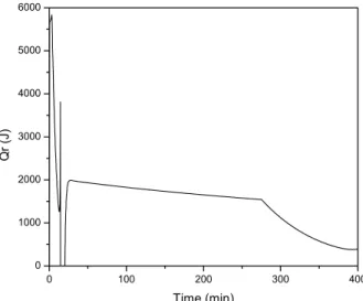
Figure 3 shows the evolution of Qr as a function of time.
A large amount of heat is released in the beginning due to the amount of monomer present in the reactor in the first stage of the process. A smooth decrease in Qr can be observed from about t=30 minutes untill the end of the semicontinuous operation.
The reactor and cooling jacket dynamic behavior are shown in Figure 4.
0 100 200 300 400 200
250 300 350 400 450
U
A
(J/
K)
Time (min)
Figure 1: UA Dynamic Behavior
0 100 200 300 400 0,0
0,2 0,4 0,6 0,8 1,0
C
o
n
v
e
rs
io
n
time(min)
Figure 2: Overall Monomer Conversion
0 100 200 300 400 0
1000 2000 3000 4000 5000 6000
Q
r
(J
)
Time (min)
Figure 3: Qr Dynamic Behavior
0 100 200 300 400 344
346 348 350 352 354 356 358 360 362 364
T
e
m
p
e
ra
tu
re
(K)
Time (min)
Temperature of the Reactor Temperature of the Jacket
Figure 4 shows that the dynamic behavior of Tr and Tj are very similar. It means that the difference (Tr – Tj) is close to a constant during the reaction. In view of what was described in the previous section, it is clear that we shall have difficulties if we try to estimate Qr and UA from equation 17. In order to overcome this shortcoming we propose the approach described in the following section.
CASCADE CALORIMETRY
If we know the value of UA then Qr can be readily estimated, independently of what happens to the difference (Tr – Tj). The same holds if we know the value of Qr and are to estimate UA. So, under the assumption of slow dynamics, we suppose that one of the variables remains constant within the interval between two consecutive temperature measurements and the other one is estimated (a typical digital acquisition unit can measure temperature every 10 seconds). Thus, one variable becomes the input of the observer of the other variable, and so on. The estimations of Qr and UA are carried out as follows:
r r
r
ˆ ˆ ˆ ˆ
Q (0) UA(1) Q (2) UA(3)
ˆ ˆ
Q (k 1) UA(k)
o o o
o o" o o"
o
where “^” stands for the estimated variable.
The selection of the initial values for both observers is very important. The estimations of Qr and UA take place independently and bad estimations of Qr leads to bad estimations of UA and so on, especially in the beginning of the reaction. We actually know that
=0. The estimation of along with
Qloss(0) is described in the following paragraphs.
)
0
(
r
Q
ˆ
U
ˆ
A
(
0
)
Estimation of ÛA(0) and Qloss(0) During Reactor Heat-Up
Othman (2000) developed a Kalman-like observer to estimate the initial values of estimated UA and Qloss from temperature measurements
during reactor heat-up. The dynamic model
employed is given by the following equation:
i i loss i feed dTr UA (Tr Tj) dt (mCp)r F Cp Q (T Tr) (mCp)r (mCp)r dQloss dUA
0, 0, y Tr
dt dt ° ° ° ° ° ® ° ° ° ° °¯
¦
(20)The system given above can be rewritten as follows:
0 Tj Tr / mCp 1/ mCp
Tr Tr
UA 0 0 0 UA
Qloss
Qloss 0 0 0
ª º
ª º « »ª
« » « »«
« » « »«¬ »¼
¬ ¼ ¬ ¼
º » (21)
This system has the form:
x(t) A u, y x(t)
y(t) Cx(t) ° ® °¯ (22)
where, x=[Tr UA Qloss]T, C=[1 0 0],
1 2
0 f f
A 0 0 0
0 0 0
ª º « » « » « » ¬ ¼ , 1
Tr Tj mCp f and 2 1 f mCpA Kalman-like observer can be used to estimate the different states. The Kalman-like observer takes the following form:
1 T
T T
ˆ ˆ ˆ
x(t) A u, y x(t) S C Cx(t) y
S S A S S A C C
T
T T T T
° ®
° T
¯
(23)
The second differential equation is the Ricatti equation that must be solved simultaneously with the estimated state differential equations. In order to
avoid the inversion of ST in the corrective term, we
denote R= ST-1, therefore, R is also a symmetric
matrix. The relation between ST and R is given
by: 1 1 R R R
ST (24)
Substitution of equation 24 in equation 23 gives:
T
T T
ˆ ˆ ˆ
x(t) A u, y x(t) RC Cx(t) y
R R RA AR RC CR
° ®
° T
¯
(25)
a d e
R d b f
e f c
ª º
« »
« »
« »
¬ ¼
(26)
the second equation in system 25 gives rise to the following six differential equation:
2
1 2
2 2
1 2
1 2
a a 2df 2ef a
b b d
c c e
d d bf ff ad
e e ff cf ae
f f e
T
° ° T ° °
T °° ®
° T
°
° T
° ° T
(27)
°¯
The matrix R is generally initialized at the identity matrix. The final observer of UA and Qloss:
j r
r r
r r r r
T T 1 ˆ
ˆ ˆ ˆ
T UA Qloss a(T
mCp mCp
ˆ
ˆ ˆ ˆ
UA d(T T ), Qloss e(T T )
§ ·
° ¨ ¸
© ¹
°° ®
°
° °¯
r
T )
(28)
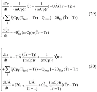
In order to decouple the variables UA and Qloss, the jacket is heated by steps. The steps of jacket temperature and the reactor temperature is shown in Figure 5.
Figure 5 shows that the difference (Tr–Tj) varies strongly with time except at the end of each step. As a result, a temporary loss of observability is expected as it is actually seen in Figures 6 and 7.
0 20 40 60 80
290 300 310 320 330 340 350 360
T
e
m
p
e
ra
tu
re
(K)
Tim e (m in) Reactor Tem perature Jacket Tem perature
Figure 5: Temperature Steps on the Jacket
100 00 20 40 60 80 1 100
200 300 400 500
00
U
A
(
J
/K
)
Time (min)
UA simulated UA estimated
Figure 6: Simulated and Estimated UA
and Reactor Temperature Dynamic Behavior
0 20 40 60 80
-100 0 100 200 300 400 500
100
Q
lo
ss
(J)
Time (min) Qloss simulated Qloss estimated
Despite the fact that the estimations take a while before converging to the simulated value, it can be seen from Figures 6 and 7 that UA and Qloss are accurately determined at the end of the reactor heat-up. These are the initial values of the cascade
calorimetry along with Qˆr(0)=0.
The impact of the term Qloss on the estimations was investigated in this work. The model employed by the cascade calorimetry assumed Qloss(t)=Qloss(0) throughout the reaction, while the model used to simulate reactor dynamics assumed a variable Qloss term.
The design of the cascade calorimetry is described in the next section.
A CASCADE OF HIGH-GAIN OBSERVERS
From equation 11 we propose the following high-gain observers to estimate Qr and UA, respectively:
i i feed loss Qr i
2 Qr
dTr 1 ˆ 1 ˆ ˆ
Qr [ UA(Tr Tj)
dt (mCp)r (mCp)r
ˆ F Cp (T Tr) Q ] 2 (Tr Tr)
ˆ
dQr ˆ
(mCp)r(Tr Tr) dt
°
° °
° T
® ° ° °
T
° ¯
¦
(29)
i i feed loss UA i
2 UA UA
ˆ
dTr ˆ(Tr Tj) 1 ˆ UA [Qr dt (mCp)r (mCp)r
ˆ F Cp (T Tr) Q ] 2 (Tr Tr)
ˆ ˆ
dUA UA (mCp)r ˆ [2 ](Tr Tr)
ˆ ˆ
dt Tr Tj Tr Tj
°
° °
°° T ®
° ° °
T T
°
°¯
¦
(30)These high-gain observers are connected in series in order to share the estimations. At a given instant, one variable is estimated and the other one is held constant as previously described.
The observer of UA as given by equation 30 has
singularity problems at the vicinities of Tˆr#Tj.
From figure 4 it can be seen that the difference (Tˆr–
Tj) is of a few units until t#50 minutes. So we may
expect difficulties in the estimation of UA within this interval.
RESULTS AND DISCUSSIONS
The performance of the cascade calorimetry was investigated by simulations carried out in the MATLAB. In order to tuning the observers the tuning parameters were selected by trior and error. In the simulations that follows the tuning parameter of
Qr,TQr, is equal to 0.05. It was found that a variable
tuning parameter of UA, TUA, would be appropriate
to overcome the observalility singularity during the 50 initial minutes of reaction. So, during 50 minutes
TUA is kept constant and equal to 1x10⁻⁵. This is an
effort to maintain as close as possible to its
initial value. From t=50 to 70 minutes, T
A Uˆ
UA is
increased linearly to 6.5x10⁻² and then kept constant
untill t=280 minutes. From t=280 to 300 minutesTUA
is decreased linearly to 1x10⁻³ and is kept constant
untill t=400 minutes. The results are presented in Figures 8 and 9.
Figure 8 shows that the estimations are in good agreement with the simulated values. It is clear that the assumption of slow dynamics does not seem to be appropriate to describe the behavior of Qr during the batch stage. However, the strong variations in Qr coincide with constant UA and the cascade
calorimetry performs almost uniquely the
estimations of Qr for the initial 50 minutes.
The estimations of UA converge within a few
minutes asTUA takes values of the order of 10
-2
. The results show that the right tuning allows the cascade calorimetry to provide accurate estimations even in the presence of incertainties in the term Qloss.
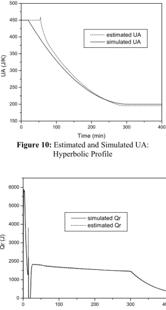
Another dynamic behavior of UA considered in this work is presented in Figure 10.
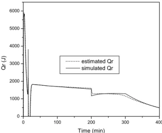
The hyperbolic profile of UA is conveniently tracked by the cascade calorimetry. The performance of the cascade calorimetry with respect to Qr is shown in Figure 11.
One major disadvantage of the ordinary open-loop calorimetry which is based on the off-line calibration of the parameter UA is the sensitivity to external disturbances. Emulsion polymerizations are essentially subjected to two typical disturbances: re-nucleation and flocculation.
0 100 200 300 400 0
1000 2000 3000 4000 5000 6000
Q
r
(J)
Time (min) estimated Qr simulated Qr
Figure 8:Estimated and Simulated Qr
0 100 200 300 400 200
250 300 350 400 450 500
U
A
(J
/K
)
Time (min)
estimated UA simulated UA
Figure 9: Estimated and Simulated UA
0 100 200 300 400 150
200 250 300 350 400 450 500
U
A
(J/
K
)
Time (min)
estimated UA simulated UA
Figure 10: Estimated and Simulated UA: Hyperbolic Profile
0 100 200 300 400 0
1000 2000 3000 4000 5000 6000
Q
r
(J
)
Time (min) simulated Qr estimated Qr
Figure 11: Estimated and Simulated Qr: Hyperbolic Profile of UA
In order to simulate the re-nucleation we proposed a 25% increase in the value of Np at t=200 minutes. The results are shown in Figures 12 and 13.
Figure 12 and 13 show that the sudden increase in the estimated value of Qr is followed by a peak in the estimated value of UA. This is a natural response of the cascade calorimetry as both observers are expected to keep the residues as small as possible. After the occurrence of the peak, the estimated value of UA tends to follow the simulated value of UA. It is evident from the results shown in Figure 13 that the observer of Qr was able to overcome the
inaccuracies verified in the estimated value of UA after the end of the semicontinuous stage.
Flocculation is characterized by a sudden
decrease in the heat generated by the reaction due to a decrease in the total number of particles. This phenomenon indicates that the surface area of the latex particles covered by emulsifier is below a critical value.
0 100 200 300 400 0
1000 2000 3000 4000 5000 6000
Q
r
(J)
Time (min) estimated Qr simulated Qr
Figure 12: Estimated and Simulated Qr under the Occurrence of Re-nucleation
0 100 200 300 400 200
250 300 350 400 450 500
U
A
(J/
K)
Time (min)
estimated UA simulated UA
Figure 13: Estimated and Simulated UA under the Occurrence of Re-nucleation
0 100 200 300 400 0
1000 2000 3000 4000 5000 6000
Q
r
(J)
Time (min) estimated Qr simulated Qr
Figure 14: Estimated and Simulated Qr under the Occurrence of Flocculation
0 100 200 300 400 200
250 300 350 400 450 500
U
A
(J/
K)
Time (min)
estimated UA simulated UA
Figure 15: Estimated and Simulated UA under the Occurrence of Flocculation
The cascade calorimetry provided accurate estimations in the occurence of flocculation. The major effect of the flocculation over the estimations is verified in the estimated value of UA, especially after end of the semicontinuous stage.
The parameter UA is indeed less sensitive to the measurements of reactor temperature than Qr. It means that the correction term is more effective in the estimations of Qr. This explains the results obtained after the occurrence of both disturbances.
CONCLUSIONS
The coupled estimation of Qr and UA was described in this work. A cascade of non-linear state observers was used to carry out the estimations. The results obtained by simulation show that this approach can provide good estimations of Qr and UA. One major advantage of cascade calorimetry is its ability to accurately estimate the variables in the presence of external disturbances. It was shown that the observers tracked the occurance of re-nucleation and flocculation in the system.
The cascade calorimetry may be regarded as a non-optimal calibration procedure. Instead of dealing with the optimization of a set of calibration parameters, the cascade calorimetry relies on tuning parameter profiles and a correction term in a closed loop sense.
NOMENCLATURE
Cpi heat capacity of substance “i”, J/kg/K
(–'Hi) heat of reaction of substance “i”, J/mol
Fi inflow rate of monomer “i”, mol/s
kpij reaction rate constant of radical “i” and
monomer “j”, L/mol/s
mi mass of substance “i” in the reactor
Mi is the residual monomer “i” in the reactor
[Mi]p concentration of monomer “i” in the
particles, mol/L
n average number of radicals per particle
Na Avogrado’s number
Np total number of polymer particles
Pi probability that an active chain in the
particle is of type “i”
Qfeed sensible heat of the feed, J/s
Qj heat exchanged through the cooling jacket,
J/s
Qloss heat loss from the reactor to the
surroundings, J/s
Qr heat generated by the polymerization, J/s
Rpi rate of polymerization of the ith monomer
in the mixture, mol/s/L
ST the unique solution of the algebric
Lyapunov equation
Tamb ambient temperature, K
Tfeed temperature of the feed, K
Tj jacket temperature, K
Tr reactor temperature, K
UA overall heat transfer coefficient, J/K/s
x state vector
xˆ
estimated state vectory measured output
Greek Letters
TUA tuning parameter of UˆA
TQr tuning parameter of Qˆr
ACKNOWLEDGEMENT
The authors thank CAPES and FAPESP for financial support. Especial thanks to Dr. Selwa Ben Amor for her assistence.
REFERENCES
Carloff, R., ProE, A. and Reichert, K., Temperature
Oscillation Calorimetry in Stirred Tank Reactors with Variable Heat Transfer, Chem. Eng. Technol., vol. 17, 406-413 (1994).
Gelb, A., Applied Optimal Estimation, The M.I.T. Press, 1974.
Fevotte, G., Barudio, I. and Guillot, J., An Adaptive Inferential Measurement Strategy for On-line Monitoring of Conversion on Polymerization Processes, Thermochimica Acta, vol. 289, 223 –
242 (1996).
Fevotte, G., McKenna, T. F., Othman, S. and Hammouri, H., Non-linear Tracking of Glass Transition Temperatures for Free Radical Emulsion Copolymers, Chem. Engng. Sci., vol. 53, no. 4, 773-786 (1998a).
Fevotte, G., McKenna, T., Othman, S. and Santos, A., A Combined Hardware/Software Sensing Approach for On-line Control of Emulsion Polymerization Processes, Comp. Chem. Eng.
Suppl., vol. 22, 443-449 (1998b).
Guinot, P., Othman, N., Févotte, G., McKenna, T.F.,
On-line monitoring of emulsion
copolymerisations using hardware sensors and calorimetry, Polymer Reaction Engineering, vol. 8, no. 2, 115-134 (2000).
Henson, M. A. and Seborg, D., Nonlinear Process Control, Prentice Hall, PTR, Upper Saddle River, New Jersey (1997).
Kravaris, C. and Kantor, J.C., Geometric Methods for Nonlinear Process Control. 1. Background, Ind. Chem. Eng. Res., vol. 29, no. 12, 2295-2310 (1990).
State Estimators for Polymer Reactors, Paper 77f, p. 486-496, 3rd Annual Polymer Producers Conference AIChE Spring Meeting, Houston (1999).
Mosebach, M. and Reichert; K, Adiabatic Reaction Calorimetry for Data Acquisition of Free-Radical Polymerizations, Journal of Applied Polymer Science, vol. 66, 673-681 (1997).
Othman, N., Stratégies Avancées de Contrôle de Composition Lors de Polymérisations Semi-Continues en Emulsion, Lyon, France, Université Claude Bernard, PhD Thesis, 2000.
Santos, A., Bentes Freire, F., Ben Amor, S., Pinto, J.
C., Giudici, R. and McKenna, T, On-line Monitoring of Emulsion Polymerization: Conductivity and “Cascade” Calorimetry, DECHEMA Monographs, vol. 137, 609-615 (2001).
Schimidt, C. U. and Reichert, K. H., Reaction Calorimetry a Contribution to Safe Operation of Exothermic Polymerizations, Chem. Eng. Sci., vol. 43, no. 8, 2133-2137 (1988).