Abstract
In this work we consider a problem in the context of the general-ized theory of thermoelasticity for a half space. The material of the half space is functionally graded in which Lamé’s modulii are functions of the vertical distance from the surface of the medium. The surface is traction free and subjected to a time dependent thermal shock. The problem was solved by using the Laplace transform method together with the perturbation technique. The obtained results are discussed and compared with the solution when Lamé’s modulii are constants. Numerical results are comput-ed and representcomput-ed graphically for the temperature, displacement and stress distributions.
Keywords
Half Space; Generalized Thermoelasticity; Perturbation method; FGM; Variable Lamé’s modulii.
Modeling of Variable Lamé’s Modulii for a FGM
Generalized Thermoelastic Half Space
1 INTRODUCTION
The theory of generalized thermoelasticity with one relaxation time was introduced by Lord and Shulman (1967). In this theory Cattaneo-Maxwell law of heat conduction replaces the conventional Fourier’s law. The heat equation associated with this theory is a hyperbolic one and hence automat-ically eliminates the paradox of infinite speeds of propagation inherent in both the uncoupled and the coupled theories of thermoelasticity. For many problems involving steep heat gradients and when short time effects are sought this theory is indispensable. Sherief and El-Maghraby (2003, 2005) solved some crack problems for this theory. Sherief and Hamza has obtained the solution of axisymmetric problems in cylindrical regions in (1994) and in spherical regions in (1996). Sherief and Ezzat (1994) have obtained the solution in the form of series. Sherief and Dhaliwal (1981) used asymptotic expansions to obtain the solution of a 1D problem and to find the locations of the wave fronts and the speed of propagation of thermoelastic waves. This theory was extended to deal with thermoelastic diffusion in (2004), micropolarity of the medium in (2005), viscoelastic effects in
Hany H. Sherief a A. M. Abd El-Latief b
aAlexandria University, Egypt, [email protected] b Alexandria University, Egypt, [email protected]
http://dx.doi.org/10.1590/1679-78252086
(2011). Sherief et.al (2010) extended this theory using fractional derivatives. Under this theory, Sherief and Abd-Ellatief (2013, 2014a, 2014b) have solved some problems.
Functionally graded materials (FGMs) are a new class of materials with the material properties varying continuously along specified directions. Due to their desirable properties, FGMs have been increasing used in modern engineering applications (Wang(2013)). For example, the functionally graded metal-ceramic composites have been used as thermal barriers or thermal shields in various applications(Lee et.al(1996), Tsukamoto(2010)). Especially, Praveen et.al. (1999) in severe tempera-ture environments, such as extremely high temperatempera-ture and thermal shock, widely potential appli-cations are opening for FGMs.
In recent years, Asgari and Akhlaghi (2009) composition of several different materials is often used in structural components in order to optimize the thermal resistance and temperature distribu-tion of structures subjected to thermal loading. Other works that consider FGM can be found in (Nahvi et.al. (2008), Zafarmand et. al. (2015), Dey et.al. (2015)).
2 FORMULATION OF THE PROBLEM
In this work, we consider a homogeneous isotropic thermoelastic solid occupying the region
x
0
composed of a FGM material whose Lamé's parameters depend on the vertical distance '' x '' from the surface. The surface of the half-space is taken to be traction free and is subjected to a thermal shock that is a function of time. We assume also that there are no body forces or heat sources inside the medium. The initial conditions are assumed to be homogenous.From the physics of the problem, it is clear that all the variables depend on x and t only. The displacement vector will thus have the form.
( , ), 0, 0
u
u x t
(1)The equation of motion is given by
2
2
u
x
t
(2)where
xx is the normal component of the stress tensor given by(
2 )
u
(3
2 )
tx
(3)where
,
are Lamé's modulii.
t is the coefficient of thermal expansion and
T
T
0 whereT is the absolute temperature, T0 is the temperature of the medium in its normal state such that
1
.2
2
2
2
(
2 )
(3
2 )
2
3
2
t
t
u
x
x
u
u
x
x
x
x
x
t
(4)where is the density. The equation of the heat conduction has the form
2 2
0 0
2 2 E
(3
2 )
tu
k
C
T
x
t
t
x
(5)where
C
E is the specific heat per unit mass in the absence of deformation, k is the thermal con-ductivity and 0 is the relaxation time. From now on, we shall take
,
in the form0
,
0a x a x
e
e
(6)
where 0, 0 and “a” are constants. Thus equations (3-5) take the form
0 0
(
2
)
e
a xu
(3
2 )
te
a xx
(7)
2
0 0 0 0
2
(
2
)
(3
2
)
a x a x
t
u
u
e
e
t
x
x
x
(8)2 2
0 0 0 0
2 2
(3
2
)
a x
E t
u
k
C
T
e
x
t
t
x
(9)We shall use the following non-dimensional variables
' ' 2 ' 2
0 0
' ' 0 0 0 0
0 0 0 0
,
'
,
,
,
'
/
(3
2
)
2
,
,
,
2
2
t E
x
c x
u
c u
t
c
t
c
a
a c
ρ
c
c
ρ
k
Using the above non-dimensional variables, equations (7)-(9) take the form
a x
u
e
x
(10)2
2
a x
u
u
e
t
x
x
2 2
0
2 2
a x
u
e
x
t
t
x
(12)The remaining components of the stress tensor are given by:
2 2
(
2)
a x yy zzu
e
x
(13)0
xy xz yz
(14)where 2 2
0
( 3
02
0)
t/ (
02
0)
T
k
, 2 0 00
(
2
)
We assume that the boundary conditions have the form
(0 , )
t
f t
( ) ,
( , ) 0 ,
t
t
0
(15)(0 , )
t
( , ) 0 ,
t
t
0
(16)where f(t) is a known function of t
3 SOLUTION IN THE LAPLACE TRANSFORM DOMAIN
Applying the Laplace transform with parameter s defined by the relation
0
( , )
s t( , )
f x s
e
f x t d t
to both sides of equations (10)-(13), we get the following equations
a x
u
e
x
(17)2
a x
u
e
s u
x
x
(18)
2
2 0 2
a x
u
s
s
e
x
x
(19)2 2
(
2)
a x yy zzu
e
x
(20)(0) (1) 2 (2)
...
a
a
(0) (1) 2 (2)
...
u
u
au
a u
(0) (1) 2 (2)
...
a
a
where ( ) ( )
and
i i
u
are functions to be determined, i = 0, 1, …Equations (18-19) gives, upon equating the coefficients of “a ” in both sides up to order 1
2 (0) (0)
2 (0) 2
u
s u
x
x
(21)2 (1) (1) (0)
2 (1) 2 (0) (0)
2
u
u
s u
x s u
x
x
x
(22)2 (0) (0)
2 (0)
0
2
(
)
u
s
s
x
x
(23)2 (1) (1) (0)
2 (1) 2
0 0
2
(
)
(
)
u
u
s
s
x s
s
x
x
x
(24)Using expansion of equation (17), we obtain
(0)
(0)
u
(0)x
(25)(1)
(1)
u
(1) (0)x
x
(26)Eliminating
(0) between equations (21) and (23), we get
2 3
(0)0 0
(1
) (1
) (1
)
0
4 2
D
D
s
s
s
s
s
u
(27)where
D
x
The general solution of equation (27) which is bounded at infinity can be written as
1 2
(0)
1 1 2 2
k x k x
u
k A e
k A e
(28)4 2 2 3
0 0
(1
)(1
)
(1
)
0
k
k
s
s s
s
s
From equations (21) and (28), we get
1 2
(0) 2 2 2 2
1
(
1)
2(
2)
k x k x
A
k
s
e
A
k
s
e
(29)
The boundary conditions (15-16) give
(0)
( ) , at
0
f s
x
(30a)(1)
0, at
x
0
(30b)(0)
(0)
0, at
0
u
x
x
(30c) (1) (1)0, at
0
u
x
x
(30d)In order to determine
A A
1,
2 we shall use the boundary conditions (30a), (30c) to obtain1 2 2 2
1 2
( )
f s
A
A
k
k
Equations (28), (29) become
1 2 (0) 1 2 2 2 1 2
[
]
( )
k x k x
k e
k e
u
f s
k
k
(31) 1 22 2 2 2
(0)
1 2
2 2
1 2
[ (
k
s
)
e
k x(
k
s
)
e
k x]
f(s)
k
k
(32)Eliminating (1)
u
between Eq. (22) and Eq. (24), we get
2 3 (1)
0 0
(0)
2 (0) 2 2
0
(1
) (1
) (1
)
2
(2
)
4 2
D
D
s
s
s
s
s
s
s
D
x
s
D
D u
(33)Substituting from equations (31-32) into the right hand side of equation (33) and factorizing the left hand side as before, we obtain
2
2
(1) 1 21 2
(
1 1)
(
2 2)
k x k x
2 2
where
2 2 2 2 2 2 2
1 1 0 1 1 1 1 0 1 1
2 2 2 2 2 2 2
2 2 0 2 1 2 2 0 2 1
2
,
2
2
,
2
C
k
s
s
s
k
A
E
k s
s
k
s
A
C
k
s
s
s
k
A E
k
s
s
k
s
A
The solution of the above non homogenous differential equation takes the form
1 2 1 2
(1) 2 2
1 2
(
1 1)
(
2 2)
k x k x k x k x
B e
B e
F x
G x e
F x
G x e
(35)
where B1 and B2 are unknown parameters depending on s while the remaining parameters, due to the particular solution, are given by
2 2
1 1 2
1 2 2 1 2 2 1 2 2 1
1 1 2 1 1 2 1 1 2
2 2
2 2 1
2 2 2 2 2 2 2 2 2 2
2 1 2 2 1 2 2 1 2
5
1
,
4
2
2
5
1
,
4
2
2
C
k
k
F
G
E
C
k
k
k
k
k
k
k
k
k
C
k
k
F
G
E
C
k
k
k
k
k
k
k
k
k
By the same manner the displacement differential equation takes the form
2
2
(1) 1 21 2
(
1 1)
(
2 2)
k x k x
2 2
D
k
D
k
u
H x
P e
H x
P e
(36)where
2 2 2 2 2 2 2
1 0 1 1 1 1 1 0 1
2 2 2 2 2 2 2
2 0 2 2 1 2 2 0 1
,
3
1
,
3
1
H
s
s
s
k
s
k A
P
k
s
s
s
A
H
s
s
s
k
s
k A
P
k
s
s
s
A
The solution of Eq. (36) is given by
1 2 1 2
(1) 2 2
1 2
(
1 1)
(
2 2)
k x k x k x k x
u
L e
L e
M x
N x e
M x
N x e
(37)where L1 and L2 are unknown parameters depending on s while the remaining parameters, due to the particular solution, are given by
2 2
1 1 2
1 2 2 1 2 2 1 2 2 1
1 1 2 1 1 2 1 1 2
2 2
2 2 1
2 2 2 2 2 2 2 2 2 2
2 1 2 2 1 2 2 1 2
5
1
,
4
2
2
5
1
,
4
2
2
H
k
k
M
N
P
H
k
k
k
k
k
k
k
k
k
H
k
k
M
N
P
H
k
k
k
k
k
k
k
k
k
2
2 2
1 2 0 1 0 1 1 1
1 0
1
L
s
s
N
s
s
k
B
G
k
s
s
(38a)
2
2 2
2 2 0 2 0 2 2 2
2 0
1
L
s
s
N
s
s
k
B
G
k
s
s
(38b)Substituting from Eqs. (35), (37) into the boundary conditions (30b), (30d), we obtain
2 1
B
B
(38c)1 1 2 2 1 2
k L
k L
N
N
(38d)Solving the above system, we obtain
1 2
1 2 2
2 1
G
G
B
k
k
(39)The other constants can be easily obtained from equation (38a, b,c).
Thus we have the solution in the Laplace transform domain for the temperature and displace-ment functions. The stress
can be determined from Eqs. (25-26). The solution in the physical domain can be obtained by using numerical inversion method outlined in (Honig and Hirdes (1984)). This method has been successfully used in solving many problems in the theory of thermoe-lasticity (see e.g. (Sherief and Megahed (1999)) , (Sherief and Anwar (1988))4 NUMERICAL RESULTS AND DISCUSSION
The copper material was chosen for purposes of numerical evaluations. The constants of the prob-lem are shown in table 1
k =386 W/(m K) t = 1.78 (10)-5 K-1 c
E = 381 J/(kg K) = 8886.73 0 =3.86 (10)10 kg/(m s2) 0= 7.76 (10)10 kg/(m s2) = 8954 kg/m3 T0 = 293 K
= 0.0168 0 = 0.025 s a = 0.3 m-1 b = 0.04 s
Table 1: The material constants.
The computations were carried out for different functions f(t). We have chosen the following two cases:
Case 1
1 2 2 2
0
(1
)
( )
( )
, giving
0
otherwise
bs
t
sin
t
b
b
e
f t
f t
b
f (s)
b s
Case 2
2
1
( )
( )
( ), which gives
f t
f t
H t
f (s)
s
The temperature, displacement and stress components were calculated by using the numerical method for the inversion of Laplace transform illustrated in Honig and Hirdes (1984). The FORTRAN pro-gramming language was used on a personal computer. The accuracy maintained was 5 digits for the nu-merical program.
4.2 FIGURES and Discussion
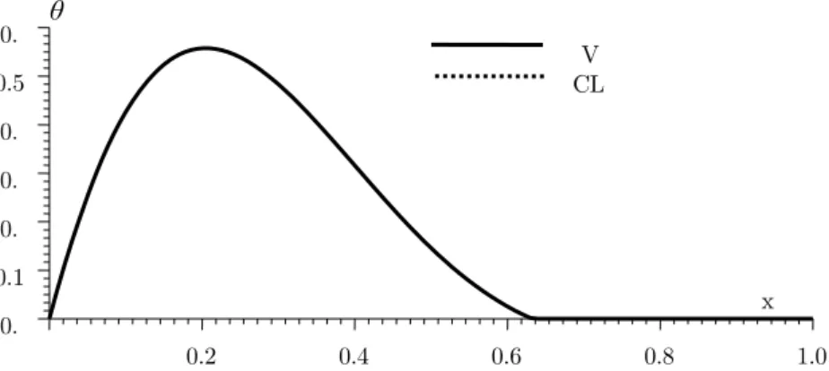
Figures (1) and (2) show the temperature distribution for t = 0.1 for cases 1 and 2, respectively. In these figures and subsequent ones the dotted lines denote the case of constant Lamé’s modulii (CL) while solid lines represent the case of variable Lamé’s modulii (VL). We note that changing of La-mé’s modulii has very small effect on the temperature profile.
Figure 1: Temperature Distribution (Case 1).
Figure 2: Temperature Distribution (Case 2).
0.2 0.4 0.6 0.8 1.0
x 0.
0.1 0. 0. 0. 0.5
0.
CL V
0. 0. 0. 0. 1.
x 0.2
0.4 0.6 0.8 1.0
CL VL
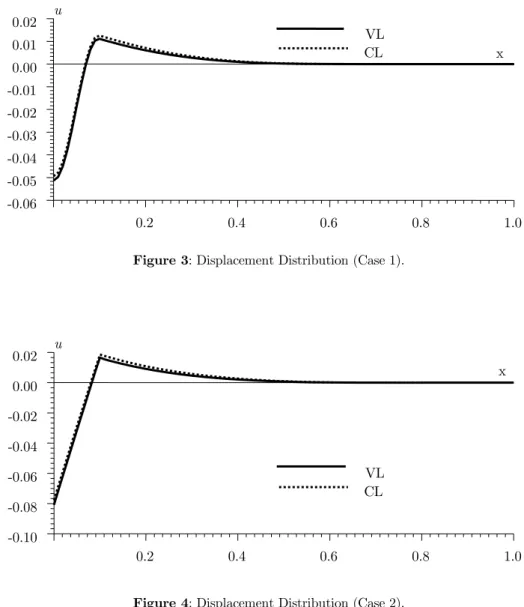
Figures (3) and (4) show the displacement distribution for t = 0.1 for cases 1 and 2, respective-ly. We note that an increase in the values of Lamé’s modulii results in an increase in the value of the displacement.
Figure 3: Displacement Distribution (Case 1).
Figure 4: Displacement Distribution (Case 2).
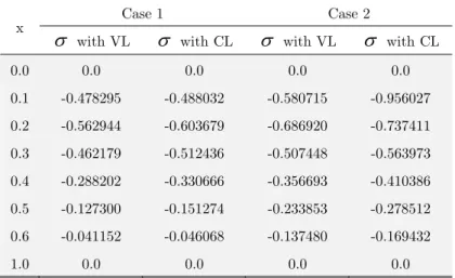
Figures (5) and (6) show the stress distribution for t = 0.1 for cases 1 and 2, respectively. We note that an increase in the values of Lamé’s modulii results in a decrease in the value of the stress component
xx .0.2 0.4 0.6 0.8 1.0
x 0.00
0.01 0.02
-0.01 -0.02 -0.03 -0.04 -0.05 -0.06
u
CL VL
0.2 0.4 0.6 0.8 1.0
x 0.00
0.02
-0.02 -0.04 -0.06 -0.08 -0.10
u
Figure 5: Stress Distribution (Case 1).
Figure 6: Stress Distribution (Case 2).
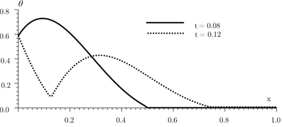
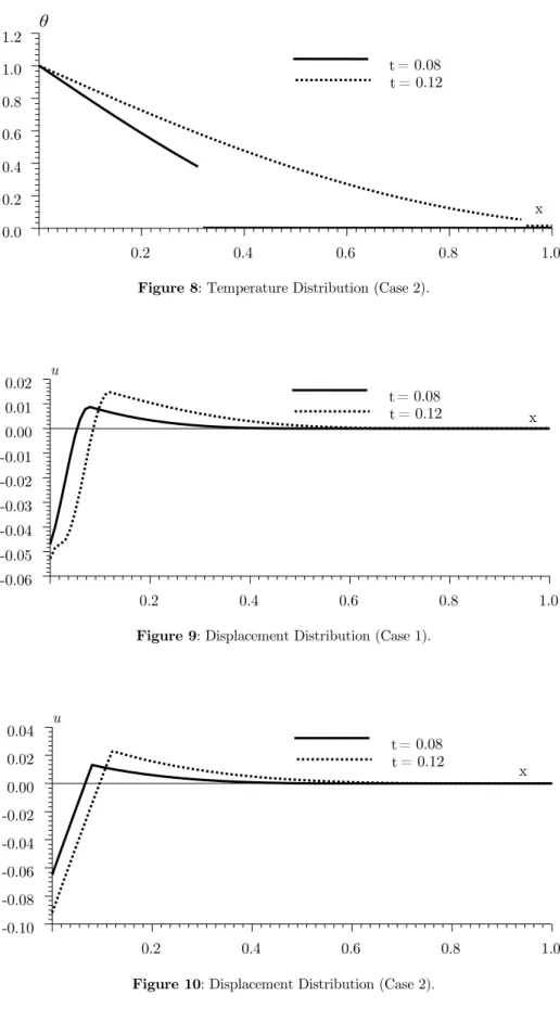
Figures (7-12) show the distributions of θ, u and σ for different times. In these figures the solid lines and the dotted lines represent t = 0.08 and t = 0.12, respectively. We note that the increase of the time results in an increase in the thermal wave penetration into the medium. The same effect is noticed for the displacement and the stress distributions.
Figure 7: Temperature Distribution (Case 1).
0.2 0.4 0.6 0.8 1.0
x 0.0
0.2 0.4 0.6 0.8
-0.2 -0.4 -0.6 -0.8
CL VL
0.2 0.4 0.6 0.8 1.0
x 0.0
0.2
-0.2
-0.4
-0.6
-0.8
-CL VL
0.2 0.4 0.6 0.8 1.0
x 0.0
0.2 0.4 0.6 0.8
Figure 8: Temperature Distribution (Case 2).
Figure 9: Displacement Distribution (Case 1).
Figure 10: Displacement Distribution (Case 2).
0.2 0.4 0.6 0.8 1.0
x 0.0
0.2 0.4 0.6 0.8 1.0 1.2
t = 0.08 t = 0.12
0.2 0.4 0.6 0.8 1.0
x 0.00
0.01 0.02
-0.01 -0.02 -0.03 -0.04 -0.05 -0.06
u
t = 0.08 t = 0.12
0.2 0.4 0.6 0.8 1.0
x 0.00
0.02 0.04
-0.02 -0.04 -0.06 -0.08 -0.10
u
Figure 11: Stress Distribution (Case 1).
Figure 12: Stress Distribution (Case 2).
Comparison between the values of all the functions are shown in tables 2-4.
x Case 1 Case 2
with VL
with CL
with VL
with CL0.0 0.000296 0.000296 1.000001 1.000001
0.1 0.425885 0.425885 0.832995 0.833987
0.2 0.557514 0.557514 0.674497 0.674486
0.3 0.483596 0.483596 0.524252 0.524261
0.4 0.316010 0.316010 0.387114 0.387143
0.5 0.145895 0.145895 0.266362 0.266402
0.6 0.045327 0.045327 0.164323 0.164365
1.0 0.000000 0.000000 0.000000 0.000000
Table 2: Temperature Values for t = 0.1.
0.2 0.4 0.6 0.8 1.0
x 0.0
0.2 0.4 0.6 0.8
-0.2 -0.4 -0.6 -0.8
t = 0.08 t = 0.12
0.2 0.4 0.6 0.8 1.0
x 0.0
0.2
-0.2
-0.4
-0.6
-0.8
x Case 1 Case 2
u with VL u with CL u with VL u with CL
0.0 -0.051336 -0.049402 -0.080899 -0.077832
0.1 0.011103 0.012565 0.016642 0.018645
0.2 0.006049 0.007109 0.009127 0.010863
0.3 0.002754 0.003371 0.004668 0.005794
0.4 0.000968 0.001236 0.002083 0.002696
0.5 0.000210 0.000280 0.000718 0.000968
0.6 0.000008 0.000011 0.000099 0.000139
1.0 0.000000 0.000000 0.000000 0.000000
Table 3: Displacement Values for t = 0.1.
x Case 1 Case 2
with VL
with CL
with VL
with CL0.0 0.0 0.0 0.0 0.0
0.1 -0.478295 -0.488032 -0.580715 -0.956027
0.2 -0.562944 -0.603679 -0.686920 -0.737411
0.3 -0.462179 -0.512436 -0.507448 -0.563973
0.4 -0.288202 -0.330666 -0.356693 -0.410386
0.5 -0.127300 -0.151274 -0.233853 -0.278512
0.6 -0.041152 -0.046068 -0.137480 -0.169432
1.0 0.0 0.0 0.0 0.0
Table 4: Stress Values for t = 0.1.
As usual in dealing with problems of the theory of generalized thermoelasticity, the finite speed of wave propagation is apparent. For t = 0.1 the solution is identically zero for x > 0.6341, approx-imately, for both cases.
We note that for case 2, the temperature and stress distributions have two discontinuities. The first discontinuity is at x = 0.973 approximately while the second discontinuity is at x = 0.6341 approximately. The first discontinuity in the temperature is very small in value and does not show in the figure. The displacement distribution is continuous but has discontinuous first derivatives at the above locations. These locations are the locations of the wave fronts. These discontinuities are due to the fact that the input thermal shock f2(t) is a discontinuous function.
References
Asgari, M., Akhlaghi, M., (2009). Transient heat conduction in two-dimensional functionally graded hollow cylinder with finite length. Heat Mass Transfer 45: 1383 1392.
Dey, S., Adhikari, S., Karmakar, A., (2015). Impact response of functionally graded conical shells. Lat Am J Solids Stru. 12(1):133-152.
Honig, G., Hirdes, U., (1984). A Method For The Numerical Inversion of the Laplace Transform. J Comp Appl Math 10:113-132.
Lee, W., Stinton, D., Berndt, C., Erdogan, F., Lee, Y., Mutasim, Z., (1996). Concept of functionally graded materials for advanced thermal barrier coating applications. J Am Ceram Soc. 79: 3003–3012.
Lord H., Shulman, Y., (1967). A Generalized Dynamical Theory Of Thermo- elasticity. J Mech Phys Solid 15: 299-309.
Nahvi, H., Salehipour, H., Shahidi, A., (2008). Generalized coupled thermoelasticity of functionally graded annular disk considering the Lord–Shulman theory. Composite Structures 83:168-179.
Praveen, G., Chin, C., Reddy, J., (1999). Thermoelastic analysis of functionally graded ceramic-metal cylinder. J Eng Mech. 125: 1259–1267.
Sherief, H., Abd El-Latief, A., (2013). Effect of variable thermal conductivity on a Half-Space under the Fractional order Theory of thermoelasticity. Int J Mech Sci 74: 185-189
Sherief, H., Abd El-Latief, A., (2014a). Application of Fractional order Theory of thermoelasticity to a 1D Problem for a Half-Space. ZAMM 94: 509 – 515.
Sherief, H., Abd El-Latief, A., (2014b). Application of fractional order theory of thermoelasticity to a 2D problem for a half-space. Appl Math Computation 248: 584-592
Sherief, H., Allam, M., El-Hagary, M., (2011). Generalized theory of thermoviscoelasticity and a half-space problem. Int J Thermophys 32:1271–1295
Sherief, H., Anwar, M., (1988). A problem in generalized thermoelasticity for an infinitely long annular cylinder, Int. j. engng. sci 26: 301-306
Sherief, H., Dhaliwal, R., (1981). A generalized one-dimensional thermal shock problem for small times. J Thermal Stresses 4: 407–420.
Sherief, H., El-Maghraby, N., (2003). An internal pennyshaped crack in an infinite thermoelastic solid. J Thermal Stresses 26: 333–352
Sherief, H., El-Maghraby, N., (2005). A mode-I crack problem for an infinite space in generalized thermoelasticity. J Thermal Stresses 28: 465–484
Sherief, H., El-sayed, A., Abd El-Latief, A. (2010) Fractional order theory of thermoelasticity. Int J Solids Structures 47: 269-275.
Sherief, H., Ezzat, M., (1994). Solution of the generalized problem of thermoelasticity in the form of series of func-tions. J Thermal Stresses 17: 75–95
Sherief, H., Hamza, F., (1994). Generalized thermoelastic problem of a thick plate under axisymmetric temperature distribution. J Thermal Stresses 17: 435–452
Sherief, H., Hamza, F., (1996). Generalized two-dimensional thermoelastic problems in spherical regions under ax-isymmetric distributions. J Thermal Stresses 19: 55–76
Sherief, H., Hamza, F., El-Sayed, A., (2005). Theory of generalized micropolar thermoelasticity and an axisymmetric half-space problem. J. Thermal Stresses 28: 409-437.
Sherief, H., Megahed, F., (1999). A two-dimensional thermoelasticity problem for a half space subjected to heat sources, Int. j. solids struct. 36: 1369-1382
Tsukamoto, H., (2010). Design of functionally graded thermal barrier coatings based on a nonlinear micromechanical approach. Comput Mater Sci. 50: 429–436.
Wang, H., (2013). An effective approach for transient thermal analysis in a functionally graded hollow cylinder. Int J Heat Mass Transfer 67: 499–505.