A new ensemble-based consistency test for the Community Earth System Model

(1)

GMDD

8, 3823–3859, 2015

A new ensemble-based consistency test for the Community Earth

System Model

A. H. Baker et al.

Title Page

Abstract Introduction

Conclusions References

Tables Figures

◭ ◮

Back Close

Full Screen / Esc

Printer-friendly Version

Interactive Discussion

Discussion

P

a

per

|

Discussion

P

a

per

|

Discussion

P

a

per

|

Discussion

P

a

per

|

Geosci. Model Dev. Discuss., 8, 3823–3859, 2015 www.geosci-model-dev-discuss.net/8/3823/2015/ doi:10.5194/gmdd-8-3823-2015

This discussion paper is/has been under review for the journal Geoscientific Model Development (GMD). Please refer to the corresponding final paper in GMD if available.

A new ensemble-based consistency test

for the Community Earth System Model

A. H. Baker, D. M. Hammerling, M. N. Levy, H. Xu, J. M. Dennis, B. E. Eaton, J. Edwards, C. Hannay, S. A. Mickelson, R. B. Neale, D. Nychka,

J. Shollenberger, J. Tribbia, M. Vertenstein, and D. Williamson

The National Center for Atmospheric Research, Boulder, CO, USA

Received: 15 April 2015 – Accepted: 16 April 2015 – Published: 8 May 2015

Correspondence to: A. H. Baker (abaker@ucar.edu)

Published by Copernicus Publications on behalf of the European Geosciences Union.

(2)

GMDD

8, 3823–3859, 2015

System Model

A. H. Baker et al.

Title Page

Tables Figures

◭ ◮

Back Close

Full Screen / Esc

Discussion

P

a

per

|

Discussion

P

a

per

|

Discussion

P

a

per

|

Discussion

P

a

per

|

Abstract

Climate simulations codes, such as the Community Earth System Model (CESM), are especially complex and continually evolving. Their on-going state of development re-quires frequent software verification in the form of quality assurance to both preserve the quality of the code and instill model confidence. To formalize and simplify this

previ-5

ously subjective and computationally-expensive aspect of the verification process, we have developed a new tool for evaluating climate consistency. Because an ensemble of simulations allows us to gauge the natural variability of the model’s climate, our new tool uses an ensemble approach for consistency testing. In particular, an ensemble of CESM climate runs is created, from which we obtain a statistical distribution that can

10

be used to determine whether a new climate run is statistically distinguishable from the original ensemble. The CESM Ensemble Consistency Test, referred to as CESM-ECT, is objective in nature and accessible to CESM developers and users. The tool has proven its utility in detecting errors in software and hardware environments and providing rapid feedback to model developers.

15

1 Introduction

The Community Earth System Model (CESM) is a state-of-the-art fully-coupled, global climate model whose development is centered at the National Center for Atmospheric Research (NCAR) (Hurrell et al., 2013). The Earth’s global climate is complex, and CESM is widely-used by scientists around the world to further our understanding of

20

the future, present and past states of the climate system. For large simulation models such as CESM, verification and validation are critical to establishing and maintaining a model’s credibility, particularly when the model is used to make decisions (e.g., Car-son II, 2002). Note that differences in interpretation exist among scientific communities in regards to the terms verification and validation (e.g., Oberkamf and Roy, 2010).

Val-25

(3)

GMDD

8, 3823–3859, 2015

System Model

A. H. Baker et al.

Title Page

Tables Figures

◭ ◮

Back Close

Full Screen / Esc

Discussion

P

a

per

|

Discussion

P

a

per

|

Discussion

P

a

per

|

Discussion

P

a

per

|

that are being modeled. Verification involves determining whether the implementation of a model is correct and matches the intended description and assumptions for the model (see, e.g. Carson II, 2002; Sargent, 2011; Whitner and Balci, 1989; Oberkamf and Roy, 2010; Goosse et al., 2014).

Software verification necessarily requires the detection and reduction of errors or

5

“quality assurance” (Oberkamf and Roy, 2010), and we focus on this component of ver-ification for CESM. As with many scientific codes, development of CESM is on-going: features are continually added; improvements are made; software and hardware en-vironments change. The primary motivation for this work is to ensure that changes during the development life cycle of CESM do not adversely affect the simulation. In

10

particular, changes during CESM development that result in simulation output that is no longer bit-for-bit (BFB) identical to previous output data require attention to ensure that the output still produces the same climate (i.e., an error has not been introduced). Note that CESM simulations are expected to produce BFB reproducible output on the same machine and processor counts when the CESM version and parameters are

15

identical.” The approach to detecting potential errors in CESM has historically been a cumbersome process at best. For example, porting the CESM code to a new ma-chine architecture results in non-BFB model output, and the current approach is as follows. First, a climate simulation of several hundred years (typically 400) is run on the new machine. Next, data from the new simulation is analyzed and compared to data

20

from the same simulation run on a “trusted” machine, and, lastly, all results are given to a senior climate scientist for approval. This informal process is not overly rigorous and relies largely on subjective evaluations. Further, running a simulation for hundreds of years is resource intensive, and this expense is exacerbated as the model grows larger and more complicated. Clearly a more rapid, objective, and accesible solution is

25

needed, particularly because a port of CESM to a new machine is just one example of a non-BFB change that requires quality assurance testing. Other common situations that can lead to non-BFB results include experiments with new compiler versions or optimizations, code modifications that are not expected to be climate-changing, and

(4)

GMDD

8, 3823–3859, 2015

System Model

A. H. Baker et al.

Title Page

Tables Figures

◭ ◮

Back Close

Full Screen / Esc

Discussion

P

a

per

|

Discussion

P

a

per

|

Discussion

P

a

per

|

Discussion

P

a

per

|

many new exascale-computing technologies. The lack of a straightforward metric for accessing the quality of the simulation output has limited the ability of CESM users and developers to introduce potential code modifications and performance improvements that result in non-BFB reproducibility. The need for a more quantitative solution for en-suring code quality prompted our development of a new tool for assessing the impact

5

of non-BFB changes in CESM. While verification always involves some degree of sub-jectivity and one cannot absolutely prove correctness (Carson II, 2002; Oberkamf and Roy, 2010), we aim to facilitate the detection of hardware, software, or human errors introduced into the simulation.

The quality assurance component of code verification implies that a degree of

con-10

sistency must exist (Oberkamf and Roy, 2010). Our new method evaluates climate consistency in CESM via an ensemble-based approach that simplifies and formalizes the quality assurance piece of the current verification process. In particular, the goal of our new CESM Ensemble Consistency Test tool, referred to as CESM-ECT, is to easily determine whether or not a change in a CESM simulation is statistically significant. The

15

ability of this simple tool to quickly assess changes in simulation output is a significant step forward in the pursuit of more qualitative metrics for the climate modeling com-munity. The tool has already proven invaluable in terms of providing more feedback to model developers and increasing confidence in new CESM releases. Note that we do not discuss verification of the underlying numerical model in this work, which is

con-20

sidered at other stages in the development of individual CESM components. Further, we do not address model validation, but mention that it is primarily conducted via hind-casts and comparisons to real world data, e.g., the Intergovernmental Panel on Climate Change Data Distribution Center has a large collection of observed data (IPCC Data Collection Center 2015).

25

(5)

GMDD

8, 3823–3859, 2015

System Model

A. H. Baker et al.

Title Page

Tables Figures

◭ ◮

Back Close

Full Screen / Esc

Discussion

P

a

per

|

Discussion

P

a

per

|

Discussion

P

a

per

|

Discussion

P

a

per

|

the new tool in practice. Finally, we give concluding remarks and discuss future work in Sect. 6.

2 Background

Climate science has a strong computational component, and the climate codes used in this discipline are typically complex and large in size (e.g., Easterbrook et al., 2011;

5

Pipitone and Easterbrook, 2012), making the thorough evaluation of climate model software quite challenging (Clune and Rood, 2011). In particular, the CESM code base, which has been developed over the last twenty years, currently contains about one and a half million lines of code. CESM consists of multiple geophysical component models of the atmosphere, ocean, land, sea ice, land ice, and rivers. These components can

10

all run on different grid resolutions, exchanging boundary data with each other through a central coupler. Because CESM supports a variety of spatial resolutions and time-scales, simulations can be run on both state-of-the-art supercomputers as well as on an individual scientist’s laptop. The myriad of model configurations available to the user contribute to the difficulty of exhaustive software testing (Clune and Rood, 2011;

15

Pipitone and Easterbrook, 2012). A particularly fascinating and in-depth description of the challenges of scientific software in general, and climate modeling software in particular, can be found in (Easterbrook and Johns, 2009). Furthermore, the societal importance of better understanding Earth’s climate is such that every effort must be made to verify climate codes as well as possible (e.g., Easterbrook et al., 2011).

20

In general, scientific codes are often in a near-constant state of development as new science capabilities are added and requirements change, and this is certainly true for CESM and other global climate models. However, despite the complexity of climate software, both the constant enrichment of the code base and the manner in which it has evolved over time has resulted in an overall quality of software superior to

25

that of other open-source projects (Pipitone and Easterbrook, 2012). Yet the pace of evolution of the code requires that issues of correctness, reproducibility and software

(6)

GMDD

8, 3823–3859, 2015

System Model

A. H. Baker et al.

Title Page

Tables Figures

◭ ◮

Back Close

Full Screen / Esc

Discussion

P

a

per

|

Discussion

P

a

per

|

Discussion

P

a

per

|

Discussion

P

a

per

|

quality are frequently being addressed. Coarse-grained testing is a common practice in climate modeling, and this global approach is useful for detecting the existence of errors in the software or input stack or the software and hardware environment (Clune and Rood, 2011). This approach does not offer information as to the source of the error, but rather as to whether or not one may exist. The goal of coarse-grained testing is

5

not to prove correctness, but to point out potential incorrectness. Fine-grained testing is needed to identify the source of errors, and typically occurs within the individual CESM component models. Our focus in this work is on a coarse-grained approach to software quality assurance, and for climate models, this global approach typically takes the form of analysis of simulation output (Easterbrook and Johns, 2009). Visualizations

10

of model output are commonly examined by climate scientists, and achieving bit-for-bit (BFB) identical results has been quite important to the climate community (Easterbrook and Johns, 2009; Pipitone and Easterbrook, 2012). If changes in the source code or software and hardware environment yield BFB results to the previous version, then this verification step is trivial. However, depending on the nature of the change, achieving

15

BFB results from one run to the next is not always possible. For example, in the context of porting the code to a new machine architecture, machine-rounding level changes can propagate rapidly in a climate model (Rosinski and Williamson, 1997). In fact, changes in hardware, software stack, compiler version, and CESM source code can all cause round-o_fflevel or larger changes in the model simulation results, and the emergence

20

of some heterogeneous computing technologies inhibit BFB reproducibility as well. Some of the difficulties caused by differences due to truncation and rounding in cli-mate codes that result in non-BFB simulation data are discussed in (Clune and Rood, 2011). In particular, the authors cite the need for determining acceptable error toler-ances and the concern that seemingly minor software changes can result in a different

25

(7)

GMDD

8, 3823–3859, 2015

System Model

A. H. Baker et al.

Title Page

Tables Figures

◭ ◮

Back Close

Full Screen / Esc

Discussion

P

a

per

|

Discussion

P

a

per

|

Discussion

P

a

per

|

Discussion

P

a

per

|

of a small perturbation in the atmospheric temperature after several days. However, this test is no longer applicable to the atmospheric component of CESM, called the Community Atmosphere Model (CAM), because the parameterizations in CAM5 are ill-conditioned in the sense that small perturbations in the input produce large pertur-bations in the output. The result is that the tolerances for rounding accumulation growth

5

are exceeded within the first few time steps. Our work builds on this idea of gauging the effects of a small temperature perturbation on the simulation, though improvements in software and hardware allow us to extend the simulation duration well beyond several days. Further, by looking only at climate signals, we relax the restriction on how the parameterizations respond.

10

3 A new method for evaluating consistency

In this section, we present and discuss a new ensemble consistency test for CESM, called CESM-ECT. We first give a broad overview, followed by more details in the sub-sequent subsections. As noted, CESM’s evolving code base and the demand to run on new machine architectures often result in data that are not BFB identical to previous

15

data. Therefore, our new tool for CESM must determine whether or not thenew config-uration (e.g., code generated with a different compiler option, on a new architecture, or after a non-climate changing code modification) should be accepted. For our purposes, we accept the new configuration if its output data is statisticallyindistinguishablefrom theoriginaldata, where theoriginaldata refers to data generated on a trusted machine

20

with an accepted version of the software stack. Our tool must:

– determine whether or not data from a new configuration is consistent with the original data

– indicate the level of confidence in its determination (e.g., false positive rate)

– be user-friendly in terms of ease of use and minimal computational requirements

25

for the end-user.

(8)

GMDD

8, 3823–3859, 2015

System Model

A. H. Baker et al.

Title Page

Tables Figures

◭ ◮

Back Close

Full Screen / Esc

Discussion

P

a

per

|

Discussion

P

a

per

|

Discussion

P

a

per

|

Discussion

P

a

per

|

Note that this new tool takes a coarse-grained approach to detecting statistical diff er-ences. Its purpose is not to isolate the source of an inconsistency, but rather to indicate the likelihood that one exists. To this end, the CESM-ECT tool works as follows. The first step requires the creation of an ensemble of simulations in an accepted environment representing the original data. The second step uses the ensemble data to determine

5

the statistical distributions that describe the original data. Next, several simulations rep-resenting the new data are obtained. And finally, a determination is made as to whether the new data is statistically similar to the original ensemble data.

3.1 Preliminaries

CESM data are written to “history” files in time slices in NetCDF format for

post-10

processing analysis. Data in history files are single-precision (by default). For this ini-tial work, we focus on history data from the Community Atmosphere Model (CAM) component in CESM, which is actively developed at NCAR. We chose to begin with CAM because the time-scales for changes propagating through the atmosphere are relatively short compared to the longer time-scales of other components, such as the

15

ocean, ice, or land models. Further, the set of CAM global output variables is diverse, and the default number for our CESM configuration (detailed in the next section) is on the order of 130. An error in CAM would certainly a_ffect the other component models in fully-coupled CESM situations; however, we cannot assume that CAM data passing CESM-ECT implies that the remaining components would also pass. Data from other

20

components (e.g. ocean, ice, and land) will be addressed in future work, though we give an example in Sect. 5 of detecting errors stemming from the ice component with CESM-ECT.

3.2 An ensemble method

The development of a tool like CESM-ECT necessitates the determination of error

25

(9)

sig-GMDD

8, 3823–3859, 2015

System Model

A. H. Baker et al.

Title Page

Tables Figures

◭ ◮

Back Close

Full Screen / Esc

Discussion

P

a

per

|

Discussion

P

a

per

|

Discussion

P

a

per

|

Discussion

P

a

per

|

nificant. Requiring that the difference be less than the natural variability of the climate system makes sense intuitively and is along the lines of Condition 2 in (Rosinski and Williamson, 1997). However, characterizing the natural variability is difficult with a sin-gle run of the original simulation. Therefore, we extend the sampling of the original data to an ensemble from which we can obtain a statistical distribution. An ensemble

5

refers to a collection of multiple realizations of the same model simulation, generated to represent possible states of the system (e.g., Dai et al., 2001). Generally, small pertur-bations in the initial conditions are used to generate the ensemble members, and the idea is to characterize the climate system with a representative distribution (as opposed to a single run). Ensembles are commonly used in climate modeling and weather

fore-10

casting (see, e.g., Dai et al., 2001; Zhu and Toth, 2008; von Storch and Zwiers, 2013; Zhu, 2005; Sansom et al., 2013) to enhance model confidence, indicate uncertainly, and improve predictions. For example, the ensemble in (Kay et al., 2015) was created by small perturbations to the initial temperature condition in CAM and is being used to study internal climate variability.

15

We generate our ensemble for CESM-ECT by running simulations that differ only in a random perturbation of the initial atmospheric temperature condition ofO(10−14). These perturbations grow to the size of NWP (Numerical Weather Prediction) analysis errors in a few hours. Each simulation is one-year in length, which is short enough to be computational reasonable, yet of su_fficient length to allow the e_ffects of the

per-20

turbation to propagate though the system. A perturbation of this size should not be climate-changing, and, while one year is inadequate to establish a climate, it is suf-ficient for generating the statistical distribution that we need. In particular, while the trajectories of the ensemble members will rapidly diverge due to the chaotic nonlin-earity of the model, the statistical properties of the ensemble members are expected

25

to be the same. Determining the appropriate number of ensemble members requires a balance between computational and storage costs and the quality of the distribution. The lower bound on the size is constrained by our use of Principal Component Analy-sis (PCA), which is described in the next subsection. PCA requires that the number of

(10)

GMDD

8, 3823–3859, 2015

System Model

A. H. Baker et al.

Title Page

Tables Figures

◭ ◮

Back Close

Full Screen / Esc

Discussion

P

a

per

|

Discussion

P

a

per

|

Discussion

P

a

per

|

Discussion

P

a

per

|

ensemble members be larger than the number of CAM variables. We chose an initial ensemble size, denoted byN_ens, of 151 for CESM-ECT. At this size, the coefficient of variation for each CAM variable is well under five percent, save for two variables that are known to have large distributions across the ensemble. The cost to generate the ensemble is reasonable because allN_ens, members can be run in parallel, resulting in

5

a much faster turn around time than for a single multi-century run (a single one-year simulation can run in a couple hours on less than a thousand cores). Note that, as explained further in Sect. 3.5, an ensemble is only generated for the control and not for the code to be tested. Hence, the ensemble creation does not impact the CESM-ECT user.

10

In summary, the CESM-ECT ensemble consists of N_ens ₌ 151 one-year climate simulations, denoted byE ₌{E₁,E₂,. . .,E_N

ens}, and is produced on a trusted machine

with an accepted version, model, and configuration of the climate code. The data for these one-year ensemble runs consists of annual temporal averages at each grid point for the selected grid resolution for all N_var variables, which are either two- or

three-15

dimensional. Retaining only the annual temporal averages for each variable helps to reduce the cost of storing the ensemble simulation output and has proved su_fficient for our purposes. We denote the dataset for a variableX asX ₌{x₁,x₂,. . .,x_N

X}, wherexi

is a scalar that represents the annual (temporal) average at grid pointi andN_X is the total number of grid points inX (determined by whetherX is a 2-D or 3-D variable).

20

3.3 Characterizing the ensemble data

The next stage in our process is the creation of the statistical distributions that describe the ensemble data. In particular, information collected from the ensemble simulations helps to characterize the internal variability of the climate model system. Results from new simulations (resulting from a non-BFB change) can then be compared to the

en-25

semble distribution to determine consistency.

(11)

GMDD

8, 3823–3859, 2015

System Model

A. H. Baker et al.

Title Page

Tables Figures

◭ ◮

Back Close

Full Screen / Esc

Discussion

P

a

per

|

Discussion

P

a

per

|

Discussion

P

a

per

|

Discussion

P

a

per

|

measurements supply tangible information to climate scientists that together give them an indication of the average state and variability across the ensemble. In particular, for each ensemble member m, the global area-weighted mean is calculated for each variableX across all grid points i and denoted byXm. Next, to create the RMSZ dis-tribution, recall that aZ-score is simply an indication of how many standard deviations

5

a value is from its mean. Therefore, for each variableX, at each grid pointi, we com-pare the value of x_i of ensemble member m (denoted by x_im) to the values of x_i in sub-ensembleE\m, whereE\mconsists of all the ensemble members ofE except for memberm. ThisZ-score calculation requires the computation of mean and standard deviation ofx_i at each grid pointi in thesub-ensemble E\m, which are referred to as

10

xE_i \mandσ_xE\m

i , respectively. TheZ-score for ensemble membermat each grid pointi

is then

Z_xm

i =

x_im−xE_i \m σ_xE\m

i

. (1)

To indicate the averageZ-score for ensemble memberm over all grid points, we cal-culate the root mean squaredZ-score (RMSZ) for each variableX:

15

RMSZm_X =

s

1

N_X

X

i

Z_xm

i 2

. (2)

Repeating this process for each ensemble member results in 151 RMSZ scores for

eachoutput variable. Finally, to facilitate the computation of RMSZ score for new runs, we also compute both the mean and standard deviation at each grid pointi for each variable X in ensemble E, denoted by xE_i and σ_xE

i, respectively. To summarize, the 20

first stage produces the following global mean and RMSZ information describing the

originaldata:

– N_var×N_ens global means,

(12)

GMDD

8, 3823–3859, 2015

System Model

A. H. Baker et al.

Title Page

Tables Figures

◭ ◮

Back Close

Full Screen / Esc

Discussion

P

a

per

|

Discussion

P

a

per

|

Discussion

P

a

per

|

Discussion

P

a

per

|

– N_var×N_ens RMSZ scores,

– N_var×N_X per-point mean and standard deviations, which are written to the CESM-ECT ensemble summary file.

Both the mean and RMSZ scores are of considerable value to scientists in terms of providing insight on the distribution across the control ensemble for each variable.

5

However, determining whether or not the climate in the new run is consistent with the ensemble data based on the number of variables that fall within the distribution (or other specified tolerance) is di_fficult without a linearly independent set of variables. For the CESM 1.3.x series, 134 variables are output by default for CAM. We exclude several redundant variables as well as those with zero variance across the ensemble

10

(e.g., specified variables common to all ensemble runs) from our analysis, resulting in

N_var₌120 variables total. A correlation analysis shows that many of these variables are highly correlated (>0.9). In fact, 52 variables are highly correlated in the global mean, and 43 in the RMSZ score, and 16 pairs are common to both. Determining objective and statistically-motivated criteria (such as false positive rates) necessitated

15

a transformation of our variable-based data to a linearly independent data space. We use Principal Component Analysis (PCA), a popular tool in data analysis, to determine the orthogonal transform needed to convert the ensemble variable values into a set of principal component scores. The principal components are orthogonal and indicate the directions in which there is the most variance, i.e. in which the data is the most

20

“spread out”, thereby exposing underlying structure in the data that might otherwise be overlooked (e.g., Shlens, 2014). A second well-known advantage of PCA is that most of the variance in the system ends up being represented by many fewer components than the original number of variables, which simplifies analysis, particularly when there are large number of variables.

25

(13)

GMDD

8, 3823–3859, 2015

System Model

A. H. Baker et al.

Title Page

Tables Figures

◭ ◮

Back Close

Full Screen / Esc

Discussion

P

a

per

|

Discussion

P

a

per

|

Discussion

P

a

per

|

Discussion

P

a

per

|

containing the global means for each variable in each ensemble member and denote the result by Vgm. Note that Nvar =120 and Nvar< Nens. Standardization of the data

involves subtracting the ensemble mean and dividing by the ensemble standard devia-tion for each variable and is important because the CAM variables have vastly different units and magnitudes. Next, we calculate the transformation matrix, or “loadings”, that

5

project the variable spaceVgm into principal component (PC) space. Loading matrix

P_gm is size (N_var×N_var) and corresponds to the eigenvector decomposition of the co-variance ofVgm, ordered such that the first PC corresponds to the largest eigenvalue

and decreasing from there. Finally, we apply the transformation toVgmto obtain the PC

scores,S_gm, for our ensemble:

10

Sgm=PgmTVgm. (3)

Now instead of using a distribution of variable global means to represent our ensem-ble, theN_var×N_ens matrix Sgm forms a distribution of PC scores that represents the

variance structure in the data. These scores have a mean of zero, so we only need to calculate the standard deviation of the ensemble scores inS_gm, which we denote by

15

σ_S

gm. To summarize, this first stage computes the following data related to the

PCA-based testing:

– N_var means of ensemble global mean values (µ_V

gm)

– N_var standard deviations of ensemble global mean values (σ_V

gm)

– N_var×N_var loadings (P_gm)

20

– N_var standard deviations of ensemble global mean scores (σ_S

gm)

which are also written to CESM-ECT ensemble summary file.

The distribution of global meanscoresfrom the ensemble, represented by the stan-dard deviations inσ_S

gm, can be used to evaluate data from a new simulation. Note that

(14)

GMDD

8, 3823–3859, 2015

System Model

A. H. Baker et al.

Title Page

Tables Figures

◭ ◮

Back Close

Full Screen / Esc

Discussion

P

a

per

|

Discussion

P

a

per

|

Discussion

P

a

per

|

Discussion

P

a

per

|

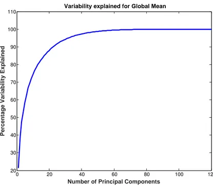
most of the variance in the data is now largely represented by a few PCs. In fact, the coefficients on the first PC explain about 21 % of the variance and the coefficients on the second explain about 17 % of the variance. Figure 1 illustrates the importance of first several PC scores. Typically the less important PC scores are neglected, and one only examines the firstN_PCcomponents in an analysis. In this work, we useN_PC ₌ 50,

5

as little additional information is gained after the first 50 PC scores.

The CESM-ECT ensemble summary file (in NetCDF format) described here is gen-erated for each CESM software tag on the Yellowstone machine at NCAR with the default compiler options (more details follow in Sect. 3.5).

3.4 Determining a pass or fail

10

The last step in the CESM-ECT procedure evaluates whether the new output data that has resulted from the non-BFB change is statistically distinguishable from the original ensemble data, as represented by the ensemble summary file. For simplicity of discus-sion, assume that we want to evaluate whether the results obtained on a new machine, Yosemite, are consistent (i.e. not statistically distinguishable) with those on

Yellow-15

stone. To do this, we collect data from a small number (N_new) of randomly selected ensemble runs on Yosemite. Variables in the new datasets are denoted byXe, where

e

X₌{xe₁,xe₂,. . .,xe_N

X}. The CESM-ECT tool then decides whether or not the output data

from simulations on Yosemite are consistent with the ensemble data and issues an overall pass or fail result.

20

CESM-ECT determines an overall pass or fail in the following manner. First, the

weighted area global means for each variable Xe in all N_new runs are calculated, Xfk (k₌1 :N_new). These new variable means are then standardized using the mean and standard deviations of the control ensemble given in the summary file (µ_V

gm andσVgm).

Second, the standardized means are converted to scores via the loading matrixP_gm

25

(15)

GMDD

8, 3823–3859, 2015

System Model

A. H. Baker et al.

Title Page

Tables Figures

◭ ◮

Back Close

Full Screen / Esc

Discussion

P

a

per

|

Discussion

P

a

per

|

Discussion

P

a

per

|

Discussion

P

a

per

|

the zero-mean scores for the ensemble in the summary file (σ_S

gm). Then for each of the

N_newYosemite simulations, the PC scores that fall outside them_σ confidence interval are tagged as a “fail” for that particular run. Finally, CESM-ECT decides whether the simulations overall on Yosemite are consistent with those on Yellowstone by counting the number of times that each PC failed at leastN_runFails runs, whereN_runFails≤N_new.

5

If at least N_pcFails PCs fail at least N_runFails runs, then CESM-ECT returns an overall “failure”.

The parametersm_σ,N_new,N_pcFails, andN_runFails are chosen to obtain a desired false positive rate. We performed an empirical simulation study and tested a variety of com-binations of parameters. We found that choosingm_σ ₌ 2 (which corresponds to the

10

95 % confidence level), N_new ₌ 3, N_pcFails ₌ 3, and N_runFails ₌ 2 yields our desired false positive rate of 0.5 %. To summarize, we run 3 simulations on Yosemite, and if at least 3 of the same PCs fail for at least 2 of these runs, then CESM-ECT issues a “failure”. We intentionally err on the conservative side by choosing a low false positive rate, hedging against the possibility that our ensemble may not be capturing all the

15

variability that we want to accept. Also note that while perturbing the initial temperature condition is a common method of ensemble creation for studying climate variability, other possibilities exist, and we are currently conducting further research on the initial ensemble composition and its representation of the range of variability, particularly in regard to compilers and machine modifications.

20

If desired, CESM-ECT also provides information on whether the variable global means and RMSZ scores fall outside of the corresponding ensemble distributions in the summary file. While this information is often of interest to climate scientists, it does not directly affect the “pass/fail” determination made by CESM-ECT, as that is based purely on the PCA testing. For each variableXe in all N_new runs, CESM-ECT can

op-25

tionally calculate theZ scores that compare the values ofxe_ik for each new run to that

(16)

GMDD

8, 3823–3859, 2015

System Model

A. H. Baker et al.

Title Page

Tables Figures

◭ ◮

Back Close

Full Screen / Esc

Discussion

P

a

per

|

Discussion

P

a

per

|

Discussion

P

a

per

|

Discussion

P

a

per

|

of the original ensembleE by

Zk

e xi =

e

x_ik−xE_i σ_xE

i

. (4)

The RMSZ scores for each variable in each run are then obtained from theZ-scores as before. TheN_newglobal means and RMSZ scores are examined independently for allN_var variables. CESM-ECT can report whether for each variableXein the new data,

5

the global mean,Xe, falls within the original ensemble distribution’s range, and, similarly for the RMSZ ofXek.

3.5 CESM-ECT software tools

Finally, we further discuss the software tools needed to test for ensemble consistency that are included in the CESM public releases (see Sect. 6 for details). Generating the

10

ensemble simulation data by setting up and running theN_ens ₌ 151 one-year simula-tions is the most compute-intensive step in this ensemble consistency-testing process. The CESM Software Engineering group generates ensembles as needed. For exam-ple, generating new ensemble simulation data is now routine when a CESM software tag is created that contains a scientific change known to alter the climate from the

pre-15

vious tag. (The frequency of such tag creation varies, but is several times a year on average). While the utility used to generate the ensemble runs is included in CESM releases, a typical end-user does not need to generate their own ensemble. Note that our consistency-testing methodology can be extended to other simulation models, and, in that case, an application-specific tool to facilitate the generation ofN_ens simulations

20

would be needed for the new application.

Whenever a new ensemble of simulations is generated, a summary file (as de-scribed in Sect. 3.3) must be created for the ensemble. The ensemble summary utility (pyEnsSum), written in parallel Python, creates a NetCDF summary for any specified number (N_ens) of output files. This step requires far less time than it takes to run the

(17)

GMDD

8, 3823–3859, 2015

System Model

A. H. Baker et al.

Title Page

Tables Figures

◭ ◮

Back Close

Full Screen / Esc

Discussion

P

a

per

|

Discussion

P

a

per

|

Discussion

P

a

per

|

Discussion

P

a

per

|

simulations themselves. As an example, generating the summary file for 151 ensemble members on 42 cores of Yellowstone takes about 20 minutes (we chose the number of cores to be equal to the number of 3-D variables). Note that the summary creation takes less than a minute if we only compute the information needed for the PCA test (i.e., exclude the most computationally expensive part, the RMSZ calculations). Each

5

CESM software tag now includes the corresponding ensemble summary file. Including the summary file in the CESM releases facilitates tracking data changes in the software life cycle and enables CESM users to run CESM-ECT without creating an ensemble of simulations themselves. Note that the storage cost for a single summary file is minor compared to the cost of storing the simulation output for the entire ensemble.

10

In addition to an ensemble summary file, our Python tool CESM-ECT (pyCECT) re-quiresN_new₌3 one-year simulations from the configuration that is to be tested. For a CESM developer or advanced user, this may mean using a development version of code with a modification that needs to be tested. For a basic CESM-user, this may mean verifying that the user’s installation of CESM on their personal machine is

accept-15

able. In either case, a simple shell script that creates one-year CESM run cases (with random initial perturbations) for this purpose is also included in CESM releases, though advanced users can certainly generate more custom simulations if desired. Regard-less, after theN_new simulations have completed, pyCECT determines whether results from the new configuration are consistent with the original ensemble data based on the

20

supplied new CAM output files and specified ensemble summary file. Then pyCECT reports whether of not the new configuration has passed or failed the consistency test, as well as which PCs in particular have passed or failed each of theN_new simulations contributing to the overall pass/fail rating. In addition, the user may assign values to the pyCECT parametersm_σ,N_new,N_pcFails, N_runFails, and N_PC via input parameters if the

25

defaults are not desired.

For clarity, Fig. 2 illustrates the workflow for the CESM-ECT process. The two Python tools are indicated by green circles. The dashed blue box delineates the work done

(18)

GMDD

8, 3823–3859, 2015

System Model

A. H. Baker et al.

Title Page

Tables Figures

◭ ◮

Back Close

Full Screen / Esc

Discussion

P

a

per

|

Discussion

P

a

per

|

Discussion

P

a

per

|

Discussion

P

a

per

|

pre-release by the CESM-software engineers. If a CESM user wants to evaluate a new configuration, the user simply executes the steps in the dashed red box.

4 Experimental studies

As noted in Sect. 1, a verification process necessarily includes some degree of sub-jectivity. The decision to designate our initial ensemble distribution as “accepted” is

5

critical to our methodology and yet, despite on-going research, we cannot (ever) be absolutely sure that this distribution is “correct” in terms of capturing all signatures that lead to the same climate. Our confidence in this initial ensemble distribution is due, in part, to the vast experience and intuition of the CESM climate scientists. However, we gain further confidence with a series of tests of trusted scenarios (i.e., scenarios

10

that we expect to produce the same climate) and verify that those scenarios pass the CESM-ECT. Similarly, we sample scenarios that we expect to be climate-changing and should, therefore, fail.

4.1 Preliminaries

The results in this work were obtained from the 1.3 release series of CESM, using

15

a present-day F compset (active atmosphere and land, data ocean, and prescribed ice concentration) and CAM5 physics. We examine 120 (out of a possible 134) variables from the CAM history files, as redundant variables and those with no variance are ex-cluded. Of the 120 variables, 78 are two-dimensional and 42 are three-dimensional variables. This spectral-element version of CAM uses a ne=30 resolution, which

cor-20

responds approximately to a 1◦global grid, containing a total of 48 602 horizontal grid-points and 30 vertical levels. Unless otherwise noted, simulations were run with 900 MPI tasks and two OpenMP threads per task on the Yellowstone machine at NCAR. The default compiler on Yellowstone for our CESM version is Intel 13.1.2 with −O2 optimization.

(19)

GMDD

8, 3823–3859, 2015

System Model

A. H. Baker et al.

Title Page

Tables Figures

◭ ◮

Back Close

Full Screen / Esc

Discussion

P

a

per

|

Discussion

P

a

per

|

Discussion

P

a

per

|

Discussion

P

a

per

|

4.2 Non-climate changing modifications

First we look at modifications that lead to non-BFB results but are not expected to be climate-changing. Such modifications include equivalent code formulations that re-sult in the reordering in floating-point arithmetic operations, thus a_ffecting the round-ing error. Two common CESM configurations that induce reorderround-ing in arithmetic

op-5

erations include removing thread-level parallelism from the model and certain com-piler changes. We expect that the following tests on Yellowstone will not be climate-changing, and thus, will be consistent with our initial ensemble distribution:

– NO-OPT: changing the Intel compiler flag to remove optimization (−O0)

– INTEL-15: changing the Intel compiler version to 15.0.0

10

– NO-THRD: compiling CAM without threading (MPI-only)

– PGI: using the CESM-supported PGI compiler (13.0)

– GNU: using the CESM-supported GNU compiler (4.8.0)

These five scenarios differ from the control run used to generate the ensemble only in the single aspect listed above. We first generateN_new₌3 simulations on Yellowstone

15

corresponding to each test scenario, where each simulation is given a perturbation selected at random from the perturbations used to create the initial ensemble. Table 2 lists the pass/fail result from pyCECT and indicates that none of these modifications caused a failure. Recall that our criteria for failure in pyCECT is that at least three PCs must fail at least two of the runs. Table 2 shows that at most two PCs failed two runs

20

for these particular test scenarios.

4.3 CAM climate-changing parameter modifications

CESM-ECT also must successfully detect changes to the simulation results that are known to be climate-changing and return a failure. To this end, climate scientists

(20)

GMDD

8, 3823–3859, 2015

System Model

A. H. Baker et al.

Title Page

Tables Figures

◭ ◮

Back Close

Full Screen / Esc

Discussion

P

a

per

|

Discussion

P

a

per

|

Discussion

P

a

per

|

Discussion

P

a

per

|

vided a list of CAM input parameters thought to affect the climate in a non-trivial man-ner. Parameter values were modified to be those intended for use with different CAM configurations (e.g. high-resolution, finite volume, etc.). We ran the following test sce-narios which were identical to the default ensemble case with the exception of the noted CAM parameter change (the name of the CAM parameter is indicated in italics,

5

and its original default value in parenthesis):

– DUST: dust emissions;dust_emis_fact=0.45(0.55)

– FACTB: wet deposition of aerosols convection factor;sol_factb_interstitial = 1.0

(0.1)

– FACTIC: wet deposition of aerosols convection factor;sol_factic_interstitial=1.0 10

(0.4)

– RH-MIN-LOW: min. relative humidity for low clouds;cldfrc_rhminl=0.85(0.8975)

– RH-MIN-HIGH: min. relative humidity for high clouds;cldfrc_rhminh=0.9(0.8)

– CLDFRC-DP: deep convection cloud fraction;cldfrc_dp1=0.14(0.10)

– UW-SH: penetrative entrainment e_fficiency – shallow;uwschu_rpen=10.0(5.0) 15

– CONV-LND: autoconversion over land in deep convection; zmconv_c0_lnd = 0.0035(0.0059)

– CONV-OCN: autoconversion over ocean in deep convection;zmconv_c0_ocn = 0.0035(0.045)

– NU-P: hyperviscosity for layer thickness (vertical lagrangian dynamics);nu_p = 20

1.0×10−14 (1.0×10−15)

(21)

GMDD

8, 3823–3859, 2015

System Model

A. H. Baker et al.

Title Page

Tables Figures

◭ ◮

Back Close

Full Screen / Esc

Discussion

P

a

per

|

Discussion

P

a

per

|

Discussion

P

a

per

|

Discussion

P

a

per

|

From Table 1, most of these tests fail by a lot more than 3 PCs, indicating that the new simulation data is quite different from the original ensemble data. However, contrary to our initial expectations, one scenario was found to be consistent and passed. Upon further investigation, the change caused by NU likely did affect some aspects of the climate in a way that would not be detected by the test. The issue is that modifications

5

to NU cause changes to the small-scales (but not to the mean of the field the diffusion is applied to) and generally affect the extremes of climate variables (such as precipita-tion). Because CESM-ECT looks at variable annual-global means, the “pass” result is not entirely surprising as errors in small-scale behavior are unlikely to be detected in a yearly global mean. Developing the capability to detect the influence of small-scale

10

events is a subject for future work.

4.4 Modifications with unknown outcome

Now we present results for simulations in which we had less confidence in the ex-pected outcome. These include running our default CESM simulation on other CESM-supported machines as well as changing to a higher level of optimization on

Yellow-15

stone (−O3). We expected that the tests on other machines supported by CESM would pass, and, for each machine, we list the machine name and location below (and give the processor and compiler type in parentheses). The affect of −O3 compiler options was not known as the CESM codebase is large and level three optimizations can be quite aggressive. The following simulations were performed:

20

– HOPPER: National Energy Research Scientific Computing Center (Cray XE6, PGI)

– EDISON: National Energy Research Scientific Computing Center (Cray XC30, Intel)

– TITAN: Oakridge National Laboratory (AMD Opteron CPUs, PGI)

25

(22)

GMDD

8, 3823–3859, 2015

System Model

A. H. Baker et al.

Title Page

Tables Figures

◭ ◮

Back Close

Full Screen / Esc

Discussion

P

a

per

|

Discussion

P

a

per

|

Discussion

P

a

per

|

Discussion

P

a

per

|

– JANUS: University of Colorado (Intel Westmere CPUs, Intel)

– BLUEWATERS: University of Illinois (Cray XE6, PGI)

– EOS: Oakridge National Laboratory (Cray XC30, Intel)

– GOLDBACH-INTEL: NCAR (Intel Xeon CPU cluster, Intel)

– GOLDBACH-PGI: NCAR (Intel Xeon CPU cluster, PGI)

5

– INTEL13-O3Yellowstone with default Intel compiler and−O3 option

– INTEL14-O3Yellowstone with Intel 14.0.2 compiler and−O3 option

– INTEL15-O3Yellowstone with Intel 15.0.0 compiler and−O3 option

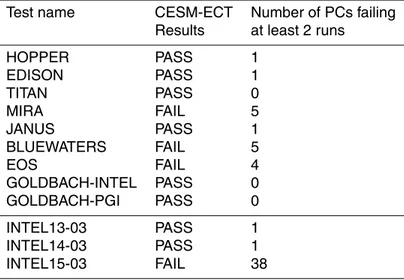
Note that we use the specified default compiler option for each CESM-supported machine. Table 3 indicates that most of the CESM-CESM-supported machine

con-10

figurations pass (the nine test scenarios above the horizontal line), and the few that fail are all near the pass/fail threshold. In other words, these machine failures are in contrast to the more egregious failures obtained by changing CAM parameters as in Table 1. However, ideally all CESM-supported machines would pass our test (assum-ing the absence of error in their hardware and software environments), and a better

15

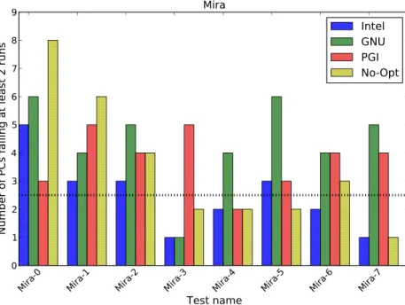
understanding of the variability introduced by the environments of other machines (i.e., not Yellowstone) is needed. Therefore, as a first step, we ran additional tests on Mira and Bluewaters with the goal of better understanding (and substantiating) the failures in Table 3. For each machine, we ran 7 more sets of three randomly perturbed simu-lations. Thus we have a total of 8 experiments each for Mira and Bluewaters, counting

20

the original in Table 3. Furthermore, we created three additional ensembles of 151 simulations based on the PGI, GNU, and NO-OPT scenarios listed in Sect. 4.2 and created a summary file for each. Thus, we can test the 8 new cases for consistency on both machines against a total of four ensembles to better understand the effect of the compiler on the consistency assessment. Results from these experiments are shown

(23)

GMDD

8, 3823–3859, 2015

System Model

A. H. Baker et al.

Title Page

Tables Figures

◭ ◮

Back Close

Full Screen / Esc

Discussion

P

a

per

|

Discussion

P

a

per

|

Discussion

P

a

per

|

Discussion

P

a

per

|

for Bluewaters and Mira in Figs. 3 and 4, respectively. Note that the Intel ensemble is the default “accepted” ensemble that we have used thus far in our experiments and the No-Opt option is also the Intel compiler (with−O0).

The results in Figs. 3 and 4 indicate that the compiler choice for the control ensem-ble on Yellowstone results in differences in the numbers of PC scores that fail each

5

individual test case. However, the overall outcome from all four control ensembles is similar in that the test results are split in terms of passes and fails, indicating that these are in fact borderline cases for CESM-ECT with the current failure criteria, which re-quires at least 3 PCs to fail at least two runs. Test scenarios that very nearly pass or fail, such as these for Bluewaters and Mira underscore the difficulty in distinguishing

10

a bug in the hardware or software from the natural variability present in the climate system. Certainly we do not expect to perfect CESM-ECT to the point where a pass or fail is a definitive indication of the absence or presence of a problem, though we have obtained a large amount of data to date that we will explore in detail to better charac-terize the effects of compiler and architecture differences on the variability. We expect

15

to report on our further analysis in future work. Finally, another difficulty for our tool is that while PCA will indicate the existence of di_fferent signatures of variability between new simulations and the ensemble, the differences detected may not necessarily be important in terms of the produced climate and the decision on whether to accept or reject that climate (e.g., because the definition of climate requires more than one year

20

and involves spatial distributions).

The last three experiments listed above and in Table 3 involve either modifying the optimization to a more agressive level (INTEL13-O3) or additionally upgrading the com-piler version (INTEL14-O3 and INTEL15-O3). Our results for INTEL15-O3 suggest that there is a compiler issue with that version. Note that because of the size of the CESM

25

code base, pinpointing a problem with a specific compiler version is time-intensive, and we find it more productive not to use that compiler.

(24)

GMDD

8, 3823–3859, 2015

System Model

A. H. Baker et al.

Title Page

Tables Figures

◭ ◮

Back Close

Full Screen / Esc

Discussion

P

a

per

|

Discussion

P

a

per

|

Discussion

P

a

per

|

Discussion

P

a

per

|

5 CESM-ECT in practice

CESM-ECT has already been successfully integrated into the CESM software engi-neering workflow. In particular, the creation of a new beta release tag in the CESM development trunk (that is not BFB with the previous tag) requires that CESM-ECT be run for the new tag on all CESM-supported platforms (e.g. the machines listed in

5

Sect. 4.4 and the supported compilers on those platforms (e.g, Intel, GNU and PGI, all with−O2, on Yellowstone). Results from these tests are kept in the CESM testing database. Failure on one or more of the test platforms signals that an error may exist in the new tag or on a particular machine, spawning an investigation and delay of the beta tag release.

10

CESM-ECT has proven its utility on numerous occasions, and we now provide sev-eral specific examples of the success of this consistency testing methodology in prac-tice. The first example concerns an early success for our ensemble-based testing methodology. The consistency test for a CESM.1.2 series beta tag test on the Mira machine failed decisively, while the consistency tests on all other platforms passed.

15

The CESM-ECT failure prompted an extensive investigation of the Mira simulation data which resulted in the discovery that the CAM energy balance was incorrect. Eventually an error was discovered in the stochastic cloud generator code that only manifested itself on big-endian systems (Mira was the only big-endian machine in the group of CESM-supported machines). Because this particular success occurred early in the

re-20

search and development stages of CESM-ECT (when we were only looking at RMSZ scores), it provided the impetus to move forward and further refine our ensemble-based consistency testing strategy.

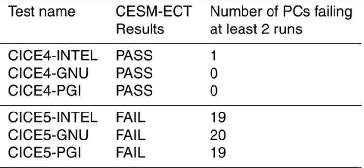
A second, more recent success for CESM-ECT was the detection of errors in a new version of the Community Ice Code (CICE). In particular, CICE5 replaced CICE4 in the

25

(25)

GMDD

8, 3823–3859, 2015

System Model

A. H. Baker et al.

Title Page

Tables Figures

◭ ◮

Back Close

Full Screen / Esc

Discussion

P

a

per

|

Discussion

P

a

per

|

Discussion

P

a

per

|

Discussion

P

a

per

|

an F compset (e.g., Sect. 4.1), which means that CICE runs in prescribed mode. Pre-scribed mode is intended for atmospheric experiments and uses the thermodynamics in the sea ice model (the dynamics are deactivated) with a pre-specified ice distribution. The CESM-ECT failures for the new development tag raised a red flag that resulted in the detection and correction of a number of errors and necessary tuning parameter

5

changes in CICE5 prescribed mode. Pre-integration component-level testing for stand-alone CICE, however, allowed errors to go undetected in prescribed mode until run with CESM-ECT. Table 4 lists the results of CESM-ECT for three test scenarios on Yellowstone (Intel, GNU, and PGI compilers) with CICE5 and CICE4, showing that the difference was quite significant.

10

Finally, CESM-ECT has been essential in the evaluation of lossy compression schemes for CESM climate data. Lossy compression schemes result in data loss when the compressed data is reconstructed (i.e., uncompressed). Evaluating the impact of the loss in precision and/or accuracy in the reconstructed data is critical to the adoption of lossy compression methods in the climate modeling community. In particular, we

ad-15

vocate for compression levels that result in reconstructed data that is not statistically distinguishable from the original data. The CESM ensemble-consistency methodology has been invaluable in making this determination (e.g., Baker et al., 2014).

6 Conclusions and future work

Software quality assurance is critical for building (and retaining) confidence in

widely-20

used scientific codes such as the Community Earth System Model. The size of the code, diversity of both the user and developer base, societal impact, and near-constant state of development for CESM require a verification technique that is easy to use and has minimal computational requirements. Further, the increasing difficulty in achieving BFB identical results due to differences across hardware and software environments

25

dictates that a verification tool determines acceptable error tolerances. This manuscript presents a ensemble-based consistency test that evaluates whether a new CESM

(26)

GMDD

8, 3823–3859, 2015

System Model

A. H. Baker et al.

Title Page

Tables Figures

◭ ◮

Back Close

Full Screen / Esc

Discussion

P

a

per

|

Discussion

P

a

per

|

Discussion

P

a

per

|

Discussion

P

a

per

|

figuration (e.g., resulting from a code modification, compiler change, or new hardware platform) is consistent with the original “accepted” (or control) configuration. The origi-nal configuration is represented by an ensemble that captures the natural variability in the modeled climate system. CESM-ECT has already been effectively incorporated into the CESM software development workflow. Our many experiments and its successes

5

in practice have increased our confidence in this methodology for detecting and reduc-ing errors in CESM. Furthermore, the utility of CESM-ECT in a number of scenarios has become apparent:

– port-verification (new CESM-supported machines);

– quality assurance for software release tags;

10

– exploration of new algorithms, solvers, compiler options;

– feedback for model developers;

– detection of errors in the software or hardware environment; and

– assessment of the effects of lossy data compression.

Despite our successes with this new consistency-testing methodology, the natural

15

variability present in the climate system makes the detection of subtle errors in CESM challenging. While no verification tool can be absolutely correct, we consider CESM-ECT in its current form to be preliminary work as many avenues remain to be explored. We are currently conducting a more detailed analysis of large ensembles from different compilers and machines in an attempt to better characterize the effects of those types

20

of perturbations. We have also begun to evaluate spatial patterns in addition to global (spatial) means, as these patterns may be revealing in such contexts as boundaries between ocean and land, and less chaotic systems like the coarse-resolution ocean. In addition, we are interested in other important climate statistics like extremes. Finally, we intend to evaluate relationships between variables in cross-covariance studies.