Newton–Raphson power flow with constant matrices: A comparison
with decoupled power flow methods
Ailson P. de Moura
a,⇑, Adriano Aron F. de Moura
baFederal University of Ceara, Campus do Pici, Caixa Postal 6001, Fortaleza, Ceara, CEP 60455-768, Brazil
bDepartment of Environmental Science and Technology, Federal Rural University of Semi-Arid, Av. Francisco Mota, 572 Bairro Costa e Silva, Mossoró-RN, CEP 59625-900, Brazil
a r t i c l e
i n f o
Article history: Received 12 June 2012
Received in revised form 30 August 2012 Accepted 18 October 2012
Available online 22 November 2012 Keywords:
Power flow Power systems Power systems planning
a b s t r a c t
This paper presents an investigation of five methods, which use constant matrices for solving the power flow problem. There are two new methods and they are based on the Newton–Raphson method with con-stant matrices of conductance and susceptance. The two aforesaid proposed methods are based on a decoupling principle, and the voltage angles and voltage magnitudes are calculated in decoupled forms. The other methods used, are XB, BX and primal. The results are compared on the basis of the convergence characteristics, number of iterations, memory requirements and the CPU times. This paper gives details of the present method’s performance in a series of practical problems on normalr/xratio systems and also on highr/xratio systems. The number of iterations and convergence characteristics of the two proposed methods, present a better performance than the decoupled versions XB, BX and primal.
Ó2012 Elsevier Ltd. All rights reserved.
1. Introduction
Many methods have been proposed to solve the problem of power flow in power systems, since the first formulation made in the 1950s. Among these methods, the decoupled methods with constant matrices are widely used. These methods are derived from the Newton–Raphson power flow method, which has become a reference point for calculating power flow due to a fast present and efficient convergence[1].
The fast decoupled power flow developed by Sttot and Alsaç (1974), has become very popular[2]. And, despite advantages such as the use of constant matrices, the method has difficulties in con-vergence on systems with ratiosr/xhigh.
In 1989, Amerongen published a paper with the BX method. This paper shows that it is preferable that the resistances are ig-nored in theB00matrix instead of theB0matrix. For normal test sys-tems, there is hardly any difference in the number of iterations, however, the new algorithm iterates faster if one or more problem-aticr/xratios are present[3].
In 1990, Monticelli et al. presented a theory that explained the performance of the decoupled versions BX and XB for the calcula-tion of power flow. They showed that the uncoupling of the Jaco-bian matrix cannot be carried out by simplifications of the expressions that represent the circuit elements. The equations must be solved with decouplings and without approximations. Therefore, this allowed to unify the study of all approaches that
fo-cus on the convergence characteristics of decoupled methods. The primal version of the decoupled method is presented in this paper [4].
Currently, several other methods are still being proposed: In 2003, two useful load flow algorithms are proposed. They are ob-tained from of the full Newton–Raphson load flow method by suc-cessively diminishing effects of the off-diagonal submatrices in the Jacobian[5]. In 2010, Moura and De Moura present a new load flow based on Newton–Raphson method. The matrices used in the method are the constants matrices of conductance and suscep-tance[6]. In 2011, Mallick et al. presents a new iterative solution technique for power flow analysis to reduce the computation com-plexity, hence time of the conventional solution techniques[7]. Several other studies in the area have recently been presented as Refs.[8–17].
As it is shown, many methods used for calculating power flow, were developed and among these methods, the decoupled meth-ods with constant matrices are widely used. The main contribution of this paper is to make a comparative study of methods with con-stant matrices, including two new power flow methods. The pro-posed methods are based on the Newton–Raphson power flow with decoupling, between the voltage magnitudes and the voltage angles with two constant matrices of conductance [G] and suscep-tance [B]. In the iterative schemes used, the update voltage angles are used for the calculations of voltage magnitudes and the update voltage magnitudes are used to calculate voltage angles. These schemes differ from the traditional Newton–Raphson power flow. The results show that the two new methods have an overall perfor-mance on the number of iterations to convergence better than the
0142-0615/$ - see front matterÓ2012 Elsevier Ltd. All rights reserved. http://dx.doi.org/10.1016/j.ijepes.2012.10.038
⇑Corresponding author. Tel.: +55 85 32413528. E-mail address:[email protected](A.P. de Moura).
Contents lists available atSciVerse ScienceDirect
Electrical Power and Energy Systems
decoupled versions XB, BX and primal. This comparative study also shows that the two proposed methods presented herewith, can be applied on normal r/xratio systems and also on high r/x ratio systems.
This paper is organized in the following manner: Firstly, the fol-lowing methods of decoupled power flow is the summarized: stan-dard (XB), modified (BX) and primal. Secondly, these proposed methods are presented in a comparative study of the decoupled methods, made with numerical results on normalr/xratio systems and also on highr/xratio systems. Final conclusions and references are contained in this paper as well.
2. Decoupled methods
2.1. XB version
The equations utilized in the fast decoupled power flow, are as follows:
D
P V
¼ ½B0
½
D
h ð1ÞD
Q V
¼ ½B00½
D
V ð2ÞThe matrices [B0] and [B00] are formed using elements of the imagi-nary part of a bus admittance matrix. The resistances are ignored in the formation of the matrix [B0]. Thus, this is the standard XB ver-sion. In the iterative scheme of the XB version, which is tested after the resolution of the voltage angles [DP] and then the solution of the voltage magnitudes [DQ] is also tested[2].
2.2. BX version
In the decoupled BX version equations, it is the same as the fast decoupled method. In the XB version, the shunts, the taps and the resistance of the branches are neglected in [B0]. In the BX version, shunts and taps are neglected in [B0]. The resistances are neglected in [B00]. In the iterative scheme of this version after each sub-solution, both [DP] and [DQ] are tested for convergence. If both mismatches reach the convergence tolerance, the procedure ends. According to the author of this iteration scheme, it avoids cyclical behavior in the calculation of voltage angles and voltage magni-tudes. This is BX version for the fast decoupled power flow[3].
2.3. Primal version
The following equations are used in decoupled primal power flow:
½
D
P ¼ ½H½D
h ð3Þ½
D
Q ¼ ½LEQ½D
V ð4Þwhere [LEQ] = [L][M][H]1[N]
The matrices [H], [L], [M] and [N], are the matrices used in the Newton–Raphson power flow for flat start in order to keep the same sparsity structure of the susceptance matrix, the fill-in ele-ments are made equal to zero in the matrix [LEQ]. These said ele-ments appear in the matrix [LEQ] due to release on [M][H]1[N]. Phase-shifts are not considered in the formation of this matrix. The iteration scheme used, is the same BX version[4].
3. Decoupled Newton–Raphson power flow with constant matrices
The development of the decoupled Newton–Raphson power flow with constant matrices is very simple and produces good re-sults on normalr/xratio systems and also on highr/xratio.
Initially, premultiplying the [DP] equations in(11)by [M][H]1
and adding the resulting equations to the [DQ] equations, leads to the following equation:
½
D
Q ½M½H1½D
P ¼ f½L ½M½H1½NgfD
Vg ð5ÞThis procedure results in the equation for calculating the voltage magnitudes.
Through a similar procedure, the calculation of voltage angles is obtained by the following equation:
½
D
P ½N½L1½D
Q ¼ f½H ½N½L1½MfD
hg ð6ÞIn the appendix Eqs.(13)–(20)the following is made: coshkmffi1 and sinhkmffi0 and, also,VkandVmequals to 1.0 p.u in the PQ buses type. The voltages magnitudes in the PV buses are kept in the duly specified values. With these stated approaches, the sub matrices [H], [M], [N] and [L] are formed exclusively with elements for the matrix of conductance [G] and matrix of susceptance [B], multiplied by voltage magnitudes of PV buses and reference bus, when the items making up these buses are being formed.
Of course, the shunts of the matrix [B] corresponding to the dimensions of the matrix [H], are not included in the calculations for the formation of this matrix. The taps are being kept in the cal-culations for the formation of all matrices. The matrices [B1], [B2], [G1] and [G2] have the following dimensions: matrix [B1] has dimensions of matrix [H], matrix [B2] has dimensions of matrix [L], matrix [G1] has dimensions of matrix [N] and matrix [G2] has dimensions of matrix [M]. Therefore, the equations of decoupled Newton–Raphson method with constant matrices (DNRCMs), are shown in the following equations:
½
D
h ¼ f½D
P ½G1½B21½D
Qg1f½B1 ½G1½B21½G2g ð7Þ½
D
V ¼ f½D
Q ½G2½B11½D
Pg1f½B2 ½G2½B11½G1g ð8Þ½hkþ1 ¼ ½hk þ ½
D
h ð9Þ½Vkþ1 ¼ ½Vk
þ ½
D
V ð10ÞThe matrix [B2] can be formed with the exclusion of PV buses from the matrix [B1], and the matrix [G2] can be constructed as the trans-posed matrix [G1] with a opposite sign.
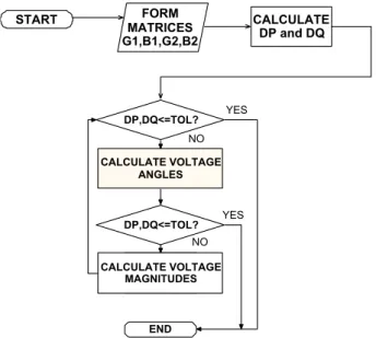
According to the scheme of iterations, the method DNRCM has two versions. In the first version, the angles of voltages are calcu-lated before the voltage magnitudes and in the second version the voltage magnitudes are calculated before the voltage angles.
The basic flowchart is the method DNRCM version 1 (DNRCMV1), shown in Fig. 1. The basic flowchart for version 2 (DNRCMV2) is similar, however, the voltage magnitude calculation is made first.
As shown inFig. 1, the scheme of iterations is different from the original method of Newton–Raphson. In the original classic scheme of the Newton–Raphson power flow, voltage magnitudes and volt-age angles of the current iteration, are always calculated using the values of previous iteration.
4. Numerical results
In this section several results are presented, in order to show the performance of the Newton–Raphson decoupled power flow with constant matrices, compared with decoupled XB, BX and pri-mal methods.
For the purpose of allowing researchers to have access to the information systems used in this study and research, the reproduc-tion of all the results shown herewith, were used with classical IEEE test systems of 14 buses, 30 buses, 57 buses and 118 buses. The computer used in these simulations, is a Semp Toshiba com-puter with Intel Core 2 Duo CPU T5550 1.83 GHz, Memory (RAM) 2 GB and 32-bit OS.
Initially, an attempt to reproduce the results presented in[4] was made. This was not entirely due to the possible usage of differ-ent computers, however, the conclusions obtained in [4] were properly confirmed. This is the primal method, which performs better than the XB version in case of systems of 30 buses and 118 buses of the IEEE.
4.1. Iteration requirements
The power flow programs based on the above specified methods written in matlab code, were duly tested on systems described above.
The first test was designed to verify the number of iterations for convergence of the methods used in this paper, when the values of the resistances of the branches are increased (scale factorsR) in transmission systems. This can be done by multiplying all the resistance branches of transmission systems by the factors of 1– 3. The results are presented onTable 1. Comparisons between re-sults of the methods DNRCMV1 and DNRCMV2 respectively, were made with the results of the methods XB, BX and primal. The tol-erance for convergence was specified at 0.001 MW/Mvar to IEEE power systems. The base power being 100 MVA.
While the results presented onTable 1shows that for the sys-tems 14, 30 and 118 buses, performs with a decoupled XB method is worst, with the largest number of iterations for convergence. Performance of the primal method is worst for the system of 57 buses. Hence, only a comparison between the decoupled methods BX, DNRCMV1 and DNRCMV2 can be summarized as follows:
– For test systems with the following cases: system of 30 buses (scale factorR= 3), system of 57 buses (scale factorR= 1) and system of 118 buses (scale factorR= 1), there is a small differ-ence in the number of iterations for convergdiffer-ence between the methods DNRCMV1, DNRCMV2 and BX.
For all the other nine cases the methods DNRCMV1 and DNRCMV2 converge in a number of iterations, less than the method BX.
The second test was designed to rigorously test the number of iterations for the convergence of power flows used in this paper, decreasing the reactance (scale factorX). The results are shown onTable 2.
According to Table 2, the methods DNRCMV1 and DNRCMV2 perform better than all other methods tested, including converging where other methods do not converge. The cases onTable 2, where the methods DNRCMV1 and DNRCMV2 are not converged, the aforesaid methods also do not converge using the classical Newton–Raphson power flow coupled, according to Eq.(11).
4.2. CPU time requirements
The CPU time and the input time requirements for the five methods recorded on the Semp Toshiba computer, are shown on Tables 3–5
The CPU time shown onTable 4, gives the CPU time taken for the iteration process only. The input time includes the time taken for the formation of the admittance matrix, Jacobian matrices and its inverse.
START
DP,DQ<=TOL?
DP,DQ<=TOL?
END CALCULATE VOLTAGE
ANGLES
CALCULATE VOLTAGE MAGNITUDES
YES
YES NO
NO FORM MATRICES G1,B1,G2,B2
CALCULATE DP and DQ
Fig. 1.Basic flowchart of method DNRCMV1.
Table 1
Iteration requirements for solutions converged from decoupled methods in trans-mission systems, are with the scale factorR.
Test system
Scale factor R
DNRCMV1 P–Q
DNRCMV2 P–Q
XB P–Q
BX P–Q
Primal P–Q
IEEE 14 1.0 6–5 5–6 8–7 9–8 8–7
2.0 6–5 5–6 11–10 10–9 9–8
3.0 9–8 8–8 21–20 11–10 9–8
IEEE 30 1.0 5–5 5–6 6–6 7–6 8–7
2.0 6–6 6–6 11–9 8–7 9–8
3.0 10–9 10–10 24–19 8–7 15–15
IEEE 57 1.0 8–8 7–8 9–9 7–7 14–14
2.0 8–8 8–8 12–11 12–12 nc
3.0 12–11 12–12 19–18 19–18 nc
IEEE 118 1.0 6–5 7–7 7–6 6–6 6–6
2.0 6–6 7–7 14–11 8–7 7–7
3.0 8–8 8–9 26–23 9–8 8–8
nc – The method does not converge in 60 iterations or diverge.
Table 2
Iteration requirements for solutions converged from decoupled methods in trans-mission systems, are with the scale factorX.
Test system
Scale factorX
DNRCMV1 P–Q
DNRCMV2 P–Q
XB P–Q
BX P–Q
Primal P–Q
IEEE 14 0.083 7–7 7–7 nc nc 29–28
0.056 16–15 16–16 nc nc nc
0.050 47–46 47–47 nc nc nc
IEEE 30 0.071 13–12 13–13 nc 22–21 nc
0.063 20–19 20–20 nc nc nc
0.056 nc nc nc nc nc
IEEE 57 0.083 12–12 12–12 nc nc nc
0.071 20–19 20–20 nc nc nc
0.063 nc nc nc nc nc
IEEE 118 0.100 12–11 12–12 nc 15–15 14–14 0.083 32–31 32–32 nc 37–37 35–35
0.071 nc nc nc nc nc
This is recorded collectively and shown onTable 3. The input time is relatively small compared to the CPU time and its time in-creases with an increasing system size. The DNRCMV1 and DNRCMV2 methods, take the longest input/output time compared to the XB, BX and primal methods, since the equations for the for-mation of the Jacobian matrix is not as straightforward as the XB
and BX methods. Comparing the input time of the five said meth-ods, the XB methods give the shortest time.
Using the CPU time onTable 4and the number of iterations for each method fromTable 1, the CPU time per iteration is computed as shown on Table 5. The DNRCMV1, DNRCMV2 and the primal methods result in an almost similar CPU time per iteration. This is much longer than the XB method. The BX method presents CPU time per iteration, being slightly longer than the XB method. The total time taken for the execution of the five methods stated above, i.e. the CPU time plus the input time, is shown onTable 6. From the results of the total execution time in Table 6, the DNRCMV1 and DNRCMV2 methods present execution times larger than the other methods.
4.3. Memory requirements
Memory requirements are compared in terms of the size of the Jacobian matrices of the five above mentioned methods, as shown onTable 7.
A numerical example to illustrate this particular item is shown as follows: We will take as example, the IEEE 14 system, The ma-trix dimensions are: DCNRCMV1 and DCNRCMV2 –B1 (1313), G1 (139), B2 (99), G2 (913), Heq (1313), Leq (99); BX and XB – B0 (1313), B00 (99); Primal – H (1313), M (913),N(139),L(99), Leq (99).
It can be observed that the XB and BX methods require the least memory, followed by the primal, DNRCMV1 and DNRCMV2 methods.
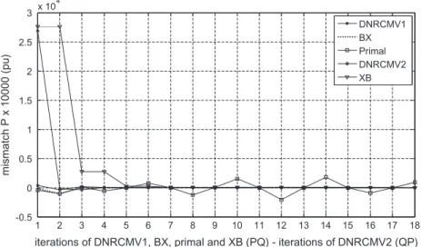
4.4. Convergence characteristics
The convergence characteristics of the duly specified five meth-ods, are described by plotting the p.u. mismatch tolerance against the iterations PQ of DNRCMV1, XB, BX and primal methods, as well as iterations QP of the DNRCMV2 method.
The graphs inFigs. 2–6, illustrate the active and reactive power mismatches from a particular bus of a power system of the IEEE. The graphics are designed to show the path convergence followed by the methods of the solution DNRCMV1, DNRCMV2, XB, BX and primal.
The graph inFig. 2, show the active power mismatches from bus 5 of the IEEE 14 bus system with the scale factorR= 1.0.
According to the figure shown above, the methods DNRCMV1 and DNRCMV2, have iterations that follow a shorter path to con-vergence compared to decoupled methods XB, BX and primal.
The graph inFig. 3shows the reactive power mismatch on bus 7 of the IEEE 14 buses system with the scale factorR= 1.0.
The graph inFig. 3shows that the second iteration of DNRCMV1 and DNRCMV2 methods, is a little further from a solution than the other methods. However, the solution path followed by the DNRCMV1 and DNRCMV2, is shorter than the methods XB, BX and primal.
The graph inFig. 4shows the power active mismatch on bus 8 of the IEEE 57 buses system with the scale factorR= 2.0.
The large difference between the methods based on Newton– Raphson with constant matrices and primal method is shown in Figs. 4 and 5. InFig. 4the residues of active power at bus 8 oscillate and the primal method cannot achieve convergence.
The graph inFig. 5shows the reactive power mismatch on bus 14 of the IEEE 57 buses system with the scale factorR= 2.0.
According toFig. 5, the oscillations of the reactive power mis-match in the primal method are quite high, while in the methods DNRCMV1 and DNRCMV2, there are no oscillations.
The graph inFig. 6, shows active power mismatch of the bar 2 in IEEE 14 buses. The scaling factor is X= 0.083. Furthermore, this
Table 3
Input time, s, requirements. Test
system
Scale factor R
Input time (s)
DNRCMV1 DNRCMV2 XB BX Primal IEEE 14 1.0 0.002 0.002 0.002 0.002 0.002 IEEE 30 1.0 0.006 0.006 0.003 0.004 0.005 IEEE 57 1.0 0.016 0.016 0.007 0.011 0.013 IEEE 118 1.0 0.055 0.055 0.023 0.041 0.042
Table 4
CPU time, s, requirements excluding input. Test
system
Scale factor R
CPU time (s)
DNRCMV1 DNRCMV2 XB BX Primal IEEE 14 1.0 0.004 0.004 0.004 0.006 0.008 IEEE 30 1.0 0.011 0.012 0.007 0.012 0.017 IEEE 57 1.0 0.050 0.040 0.026 0.033 0.088 IEEE 118 1.0 0.156 0.166 0.075 0.121 0.148
Table 5
CPU time, s, per iteration (P+Q). Test
system Scale factorR
CPU time per iteration (s)
DNRCMV1 DNRCMV2 XB BX Primal IEEE 14 1.0 0.0004 0.0004 0.0003 0.0004 0.0005 IEEE 30 1.0 0.0011 0.0011 0.0006 0.0009 0.0011 IEEE 57 1.0 0.0031 0.0026 0.0014 0.0024 0.0031 IEEE 118 1.0 0.014 0.012 0.0058 0.010 0.012
Table 6
Total execution time, s. Test
system
Scale factor R
CPU time (s)
DNRCMV1 DNRCMV2 XB BX Primal IEEE 14 1.0 0.006 0.006 0.006 0.008 0.010 IEEE 30 1.0 0.017 0.018 0.010 0.016 0.022 IEEE 57 1.0 0.066 0.056 0.033 0.044 0.101 IEEE 118 1.0 0.211 0.221 0.098 0.162 0.190
Table 7
Memory requirements. DNRCMV1 and DNRCMV2
XB BX PRIMAL
B1 – (NB-1)(NB-1) B0– (NB
-1)(NB-1)
B0– (NB
-1)(NB-1)
H– (NB-1)(NB-1) G1 – (NB-1)(NPQ) B0 0–
(NPQ)(NPQ) B0 0–
(NPQ)(NPQ)
M– (NPQ)(NB-1) B2 – (NPQ)(NPQ) N– (NB-1)(NPQ) G2 – (NPQ)(NB-1) L– (NPQ)(NPQ) Heq – (NB-1)(NB
-1)
Leq – (NPQ)(NPQ) Leq – (NPQ)(NPQ)
1 2 3 4 5 6 7 8 9 10 11 -8000
-6000 -4000 -2000 0 2000 4000 6000
iterations of DNRCMV1, BX, primal and XB (PQ) - iterations of DNRCMV2 (QP)
mismatch P x 10000 (pu)
DNRCMV1 BX Primal DNRCMV2 XB
Fig. 2.Active power mismatch on bus 6 of the 14 buses IEEE – scale factorR= 1.0.
1 2 3 4 5 6 7 8 9 10 11
-1000 0 1000 2000 3000 4000 5000 6000 7000
mismatch Q x 10000 (pu)
iterations of DNRCMV1, BX, primal and XB (PQ) - iterations of DNRCMV2 (QP) DNRCMV1 BX Primal DNRCMV2 XB
Fig. 3.Reactive power mismatch on bus 7 of the 14 buses IEEE – scale factorR= 1.0.
1 2 3 4 5 6 7 8 9 10 11 12 13 14 15 16 17 18
-0.5 0 0.5 1 1.5 2 2.5
3 x 10 4
mismatch P x 10000 (pu)
iterations of DNRCMV1, BX, primal and XB (PQ) - iterations of DNRCMV2 (QP) DNRCMV1 BX Primal DNRCMV2 XB
graphic is designed to emphasize the difference in convergence be-tween the methods DNRCMV1 and DNRCMV2 with the BX method. In the above stated graph, the BX method has a great oscillation, while the methods DNRCMV1 and DNRCMV2 converge smoothly.
5. Conclusions
This paper presented a comprehensive and comparative study between power flow methods with constant matrices. Among these methods, two new methods were presented, based on Newton–Raphson with constant matrices. Test results are analyzed regarding the number of iterations, memory requirements, CPU times and convergence characteristics. These tests have revealed the respective advantages and disadvantages of the five methods duly presented in the study.
It may be summarized that the XB and BX methods are both reliable and rapid in convergence, whereas the XB method is faster and may even fail to converge under severe ill-conditioning. The primal method was the method that obtained the worst results for convergence. DNRCMV1 and DNRCMV2 methods, present exe-cution times larger than the other methods. Memory requirements of two new methods are larger than the other decoupled methods tested. In general, the DNRCMV2 and DNRMCV1 methods, have a
performance in number of iterations for convergence better than the decoupled XB, BX and primal versions, on normalr/xratio sys-tems, as well as on highr/xratio systems.
Appendix A. Newton–Raphson power flow
Details of the algorithm of Newton–Raphson method for com-puting power flow are widely found in the literature, and readers interested in more details may consult[18].
The method is based on the solution of the Jacobian matrix:
½J
D
hD
V
¼
D
PD
Q
ð11Þ
whereJis the jacobian matrix;Dhis the vector of voltage angle cor-rections;DVis the vector of voltage magnitude corrections;Vis the voltage magnitudes vector; DPis the vector of real power mis-matches;DQis the vector of reactive power mismatches.
The Jacobian matrix can be represented as:
½J ¼ H N M L
ð12Þ
whereHis the matrix of dimensions (NPQ+NPV)(NPQ+NPV);N is the matrix of dimensions (NPQ+NPV)(NPQ);Mis the matrix of
1 2 3 4 5 6 7 8 9 10 11 12 13 14 15 16 17 18
-2.5 -2 -1.5 -1 -0.5 0 0.5 1 1.5 x 10
4
iterations of DNRCMV1, BX, primal and XB (PQ) - iterations of DNRCMV2 (QP)
mismatch Q x 10000 (pu)
DNRCMV1 BX Primal DNRCMV2 XB
Fig. 5.Reactive power mismatch on bus 14 of the 57 buses IEEE – scale factorR= 2.0.
1 2 3 4 5 6 7 8 9 10 11 12 13 14
-800 -700 -600 -500 -400 -300 -200 -100 0 100
iterations of BX and DNRCMV1 (PQ) - iterations of DNRCMV2 (QP)
mismatch P x 10 (PU)
BX DNRCMV1 DNRCMV2
dimensions (NPQ)(NPQ+NPV); L is the matrix of dimensions (NPQ)(NPQ); NPQis the number of buses type PQ; NPV is the number of buses typePV.
The elements of sub matrices [H], [N], [M] and [L] are given by
Hkk¼ V2kBkkVk X
n
m¼1
VmðGkm sinhkmBkm coshkmÞ ð13Þ
Hkm¼VkVmðGkm sinhkmBkm coshkmÞ ð14Þ
Nkm¼VkðGkm coshkmþBkm sinhkmÞ ð15Þ
Nkk¼VkGkkþ X
n
m¼1
VmðGkm coshkmþBkm sinhkmÞ ð16Þ
Mkm¼ VkVmðGkm coshkmþBkm sinhkmÞ ð17Þ
Mkk¼ V2kGkkþVk X
n
m¼1
VmðGkm coshkmþBkm sinhkmÞ ð18Þ
Lkm¼VkðGkm sinhkmBkm coshkmÞ ð19Þ
Lkk¼ VkBkkþ X
n
m¼1
VmðGkm sinhkmBkm coshkmÞ ð20Þ
The Jacobian matrix has few non-zero and Eq.(13)can be solved using bifatorization or LU factorization.
References
[1] Duncan Glover J, Sarma Mulukutla S, Overbye Thomas J. Power system analysis and design. 5th ed. Thomson Learning; 2011.
[2] Stott B, Alsaç O. Fast decoupled load flow. IEEE Trans Power Appl Syst 1974:859–69.
[3] Amerongen RAM. A general – purpose version of the fast decoupled load flow. IEEE Trans Power Syst 1989:760–70.
[4] Monticelli AJ, Garcia A, Saavedra OR. Fast decoupled load flow: hypothesis, derivations and testing. IEEE Trans Power Syst 1990:1425–31.
[5] Lee SC, Park KB. Flexible alternatives to decoupled load flows at minimal computational costs. Int J Electr Power Energy Syst 2003;25:319–26. [6] Moura AP, De Moura Adriano AF. Newton–Raphson decoupled load flow with
constant matrices of condutance and susceptance. In: 2010 9th IEEE/IAS international conference on industry applications (INDUSCON); 2010. p. 1–6. [7] Mallick Sourav, Rajan DV, Thakur SS, Acharjee P, Ghoshal SP. Development of a new algorithm for power flow analysis. Int J Electr Power Energy Syst 2011;33:1479–88.
[8] Kubba Hassan, Mokhlis Hazlie. An enhanced RCGA for a rapid and reliable load flow solution of electrical power systems. Int J Electr Power Energy Syst 2012;43:304–12.
[9] Kalesar Belal Mohammadi, Seifi Ali Reza. Fuzzy load flow in balanced and unbalanced radial distribution systems incorporating composite load model. Int J Electr Power Energy Syst 2010;32.
[10] Briceno Vicente WC, Caire R, Hadjsaid N. Probabilistic load flow for voltage assessment in radial systems with wind power. Int J Electr Power Energy Syst 2012;41:27–33.
[11] Hamouda Abdellatif, Zehar Khaled. Improved algorithm for radial distribution networks load flow solution. Int J Electr Power Energy Syst 2011;33:508–14. [12] Bo Rui, Li Fangxing, Tomsovic Kevin. Prediction of critical load levels for AC
optimal power flow dispatch model. Int J Electr Power Energy Syst 2012;42:635–43.
[13] Gallego Luis A, Padilha-Feltrin Antonio. Power flow for primary distribution networks considering uncertainty in demand and user connection. Int J Electr Power Energy Syst 2012;43:1171–8.
[14] Pereira LES, da Costa VM, Rosa ALS. Interval arithmetic in current injection power flow analysis. Int J Electr Power Energy Syst 2012;43:1106–13. [15] Yang Xiaoyu, Zhou Xiaoxin, Ma Yichen, Zhengchun Du. Asymptotic numerical
method for continuation power flow. Int J Electr Power Energy Syst 2012;43:670–9.
[16] Vinkovic Anton, Mihalic Rafael. Universal method for the modeling of the 2nd generation FACTS devices in Newton–Raphson power flow. Int J Electr Power Energy Syst 2011;33:1631–7.
[17] Yang Xiaoyu, Zhou Xiaoxin, Du Zhengchun. Efficient solution algorithms for computing fold points of power flow equations. Int J Electr Power Energy Syst 2011;33:229–35.