Interpolation strategy based on Dynamic Time Warping

UNIVERSIDADE FEDERAL DO CEAR ´A CENTRO DE CIˆENCIAS

DEPARTAMENTO DE F´ISICA

PROGRAMA DE P ´OS-GRADUAC¸ ˜AO EM F´ISICA

FELIPE GIOACHINO OPERTI

INTERPOLATION STRATEGY BASED

ON DYNAMIC TIME WARPING

FELIPE GIOACHINO OPERTI

INTERPOLATION STRATEGY BASED

ON DYNAMIC TIME WARPING

Presented by Programa de P´os-Gradua¸c˜ao em F´ısica da Universidade Federal do Cear´a, as partial requirement for the acquisition of the licence of Mestre em F´ısica. Field: Physics of Condensed Matter.

Orientador: Prof. Dr. Jos´e Soares de An-drade J´unior

FELIPE GIOACHINO OPERTI

INTERPOLATION STRATEGY BASED

ON DYNAMIC TIME WARPING

Presented by Programa de P´os-Gradua¸c˜ao em F´ısica da Universidade Federal do Cear´a, as partial requirement for the acquisition of the licence of Mestre em F´ısica. Field: Physics of Condensed Matter.

Approved in 29/01/2015

EXAMINERS

Prof. Dr. Jos´e Soares de Andrade J´unior (Orientador) Universidade Federal do Cear´a (UFC)

Dr. Erneson Alves de Oliveira Universidade Federal do Cear´a (UFC)

Prof. Dr. Liacir Dos Santos Lucena

International data for the publication Universidade Federal do Cear´a

Biblioteca Setorial de F´ısica A000p Operti, Felipe Gioachino .

Interpolation strategy based on Dynamic Time Warping / Fe-lipe Gioachino Operti. – 2015.

53 p.;il.

Disserta¸c˜ao de Mestrado - Universidade Federal do Cear´a, De-partamento de F´ısica, Programa de P´os-Gradua¸c˜ao em F´ısica, Centro de Ciˆencias, Fortaleza, 2015.

´

Area de Concentra¸c˜ao: F´ısica da Mat´eria Condensada Orienta¸c˜ao: Prof. Dr. Jos´e Soares de Andrade J´unior

1. Dijkstra’s Algorithm. 2. Optimal-Path. 3. Dynamic Time Warping. 4. Standard Linear Interpolation. 5. Dynamic Time Warping Interpolation. I.

To my parents, my family and to my

Acknowledgments

I would like to thank everyone who contributed to the thesis. In particular:

• First and foremost, my parents;

• Professor Dr. Jos´e Soares de Andrade J´unior for his orientation, his help and his support during this year and a half;

• Dr. Erneson Alves de Oliveira that with a lot of calm and patience supported me countless times;

• Rilder Pires for his help in programming;

• Samuel Morais for the many tips;

• Thiago Bento for the many discussions;

• Caleb Alves for his incentives;

• Tatiana Alonso Amor for her friendship;

• The Department of Physics (UFC), all the professors and the colleagues of the group of complex systems;

• CNPq for the financial support;

• My italian friends, Nicol´o, Simone and Alessandro for their tips;

I want to know how God created this world. I am not interested in this or that phenomenon, in

the spectrum of this or that element. I

want to know his thoughts; the rest are

details.

ABSTRACT

In oil industry, it is essential to have the knowledge of the stratified rocks’ lithology and, as consequence, where are placed the oil and the natural gases reserves, in order to efficiently drill the soil, without a major expense. In this context, the analysis of seismological data is highly relevant for the extraction of such hydrocarbons, producing predictions of profiles through reflection of mechanical waves in the soil. The image of the seismic mapping produced by wave refraction and reflection into the soil can be analysed to find geological formations of interest. In 1978, H. Sakoe et al. defined a model called Dynamic Time Warping (DTW)[23] for the local detection of similarity between two time series. We apply the Dynamic Time Warping Interpolation (DTWI) strategy to interpolate and simulate a seismic landscape formed by 129 depth-dependent sequences of length 201 using different values of known sequences m, where m = 2,3,5,9,17,33,65. For comparison, we done the same operation of interpolation using a Standard Linear Interpolation (SLI). Results show that the DTWI strategy works better than the SLI when m = 3,5,9,17, or rather when distance between the known series has the same order size of the soil layers.

LIST OF FIGURES

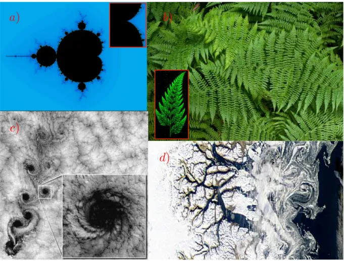
1 The Fig. ashows the Mandelbrot set with a zoom in a part of it. In Fig.

b, an image of a fern made available by the National Geographic, with a

simulation of a fern leaf. Fig. c and dare two images made available by

NASA; the first one shows a large-scale fractal motion of clouds and the

second image shows the fractal patterns of the fjords of the Greenland. p. 18

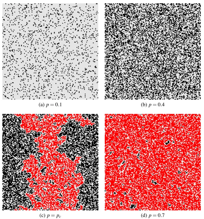
2 The figure shows four square lattice of dimension 128×128 for different values of p. The black squares are the occupied sites and the white

squares are the not occupied sites. In red are shown the clusters [18]. . p. 21

3 First neighbours of Von Neumann. The dark green represents the tree and in light green are represented the first neighbours of Von Neumann.

A tree could burn another tree only if this one is a neighbour of the first. p. 23

4 Lifetime htvi as a function of the probability of occupation for a lattice

of size sideL= 1024 for 1000 samples with Von Neumann neighbours [18]. p. 23

5 The forest fire model for a lattice of size side L = 1024 at p ∼= pc. The

trees are represented in green, the burning trees in red and the burned

trees in black [18]. . . p. 24

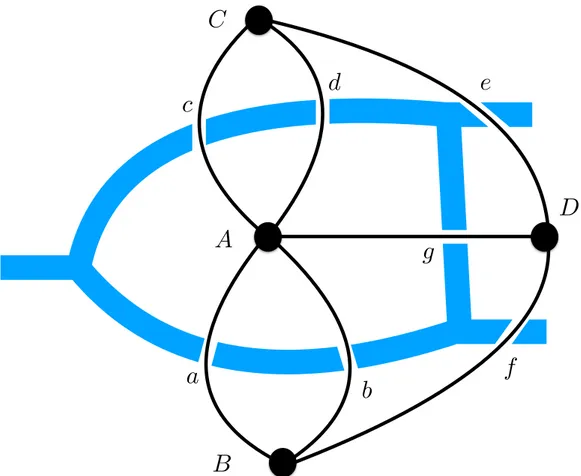
6 The Seven Bridges of K¨onigsberg. The seven bridges are represented by the letters a, b, c, d, e, f, g and the land is represented by the letters

A, B, C, D . . . p. 26

7 The Figure shows the shortest path between the source point S and the

target pointF. Every vertex is represented by a letterS, A, B, C, D, E, F, G

and it is assigned a time value for each edge. The red arrows represent

8 Example of an application of the Dijkstra’s algorithm step by step [18]. The black vertices belongs to the S set. The shaded vertices are those that have the minimum value within the Q set, where Q = V − S. The shaded edges represent the connections with the predecessors. The

algorithm will find all the shortest path among the source vertex and all

the other vertices [18]. . . p. 30

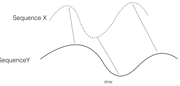
9 Alignment of two time-dependent sequencesX(t) ={xt₁, xt₂, ..., xtN}and

Y(t) ={yt1, yt2, ..., ytM}, where N, M ∈N. The grey lines represent the

correlations between the series. . . p. 32

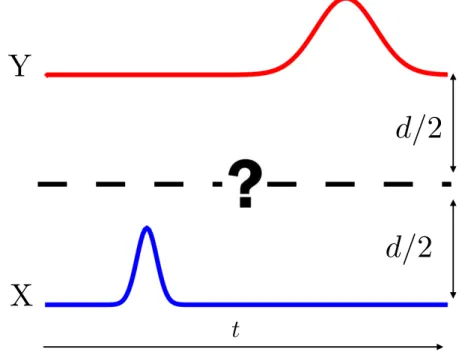
10 Two time-dependent gaussian sequencesX ={x1, x2, ..., xN}in blue and

Y ={y1, y2, ..., yN}in red, where N ∈N, separated by a distanced. The

dashed black line represents the unknown sequence to interpolate. . . . p. 33

11 Standard Linear Interpolation (SLI) between two time-dependent

gaus-sian sequences X = {x1, x2, ..., xN} in blue and Y = {y1, y2, ..., yN} in

red, where N ∈ N_{, separated by a distance d. The pink sequence} rep-resents the result of the SLI where the interpolated sequence is in the middle of X and Y. A SLI provides an interpolation where the time

flows from top to bottom or vice versa. . . p. 34

12 The figure shows the cost matrix generated starting from the two se-quences X and Y. Each site is defined by C(i, j) = |xi −yj| and the

colour scale represents the level of correlations between the two points

xi and yj of the sequences. Blue represents an high correlation and red

a low correlation.The black path represents the Optimal Warping Path

(OWP). . . p. 35

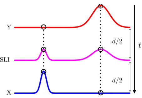
13 Dynamic Time Warping Interpolation (DTWI) between two time-dependent gaussian sequences X ={x1, x2, ..., xN} in blue and Y ={y1, y2, ..., yN}

in red, where N ∈ N_{, separated by a distance d. The green sequence} represents the result of the DTWI where the interpolated sequence is in the middle of X and Y. A DTWI provides an interpolation where the

14 Seismic data provided from WesternGeco [24]. The landscape is formed by 129 sequences made by 201 points each one. The colour scale repre-sents the variation of a characteristic of the soil. The red line reprerepre-sents

f1(y) and the blue line f2(y). I is the intensity of the seismic signal. . . p. 37

15 Sequences depth-dependent f1(y) in Fig. 15a andf2(y) in Fig. 15b. The

y represents the depth and f1(y) and f2(y) represent a characteristic of

the earth in function of the depth. . . p. 38

16 An example of the cost matrix generated by using the two sequences

f1(y) and f2(y) showed in Fig. 15a and 15b. The weight of each site is

given by c(i, j) = |f1(i)−f2(j)|, where i, j = {1,2, ..., N}. The colour

scale vary from blue (high correlation) to red (low correlation). . . p. 38

17 The second and the third conditions imply that the path at a given site could take three directions only. In order to develop the path, the blue

squares represent the predecessors of the dark green square. From the dark green square, the path may follow only one of the three directions marked by the red dashed arrows. The possible next site of the path can

be only one of the squares painted by light green. . . p. 40

18 In green the optimal warping path pk resulting from the cost matrix of

the Fig. 16, where the sequences used aref1(y) andf2(y). In light blue,

the external points of the path. . . p. 40

19 Linear Interpolation between two points of the sequencesf1(y) andf2(y) using DTWI. f1(y1) and f2(y2) are the two elements of the sequences that are correlated, where y1 and y2 are the respective depths. This

result comes from the optimal warping path. d is the distance between the two points of the sequences. dyj is the distance of the interpolated

point fi(yj) from the point f1(y1), and yj is its depth. . . p. 41

20 Interpolated landscape from seismic data using only the two series f1(y)

and f2(y) presented in Fig. 15a and 15b with DTWI. . . p. 42

21 Linear Interpolation between two points of the sequencesf1(y) andf2(y) using SLI technique. The f1(y) and f2(y) are two values of the known

sequences at the same depthy. fi(y) is the interpolated point, wheredis

the distance between the known sequences anddi is the distance between

22 DTWI applied to interpolate the lithology of the stratified rocks, starting from a real landscape (Fig. 14). The m value represents the number of known sequences, m = {2,3,5,9,17,33,65}. Each figure represents the interpolated landscape with a different value of m. I is the intensity of

the seismic signal. The dashed black lines represent the known sequences whenm= 2,3,5,9. Whenm = 17,33,65 there are not dashed black lines

because the distance among them is too small to be represented. . . p. 45

23 SLI technique applied to interpolate the lithology of the stratified rocks, starting from a real landscape (Fig. 14). The m value represents the number of known sequences, m={2,3,5,9,17,33,65}. Each figure rep-resents the interpolated landscape with a different value of m. I is the intensity of the seismic signal. The dashed black lines represent the known sequences when m= 2,3,5,9. Whenm= 17,33,65 there are not dashed black lines because the distance among them is too small to be

represented. . . p. 46

24 The graph represents the square errorErr2

for the DTWI interpolation strategy Err2

DT W I in red and for the SLI techniques Err

2

SLI in green in

function of the number of known sequences min a logarithmic scale. For

m = 3,5,9,17 the Err2

DT W I is less than the Err

2

SLI. . . p. 47

25 The figure represents the percentage difference %Dif fDT W I,SLI between

Err2

SLI and Err

2

DT W I for the value of m = 3,5,9,17,33. For the fourth

one, the DTWI strategy is ∼20% better than the SLI technique. . . p. 48

26 For m = 3,5,9,17, the figures represent the variation of the Err2

DT W I

and the Err2

SLI in function of the distance d from the first sequence,

in other words, for the cases where the DTWI is better than the SLI technique. The blue vertical lines represent the known sequences when

m = 3,5,9. When m= 17 there are not blue lines because the distance

LIST OF ACRONYMS

ABNT Associa¸c˜ao Brasileira de Normas T´ecnicas

CNPq Conselho Nacional de Desenvolvimento Cient´ıfico e Tecnol´ogico

OP Optimal path

OPW Optimal path warping

DTW Dynamic Time Warping

SLI Standard Linear Interpolation

SUMMARY

1 INTRODUCTION p. 15

2 THEORETICAL FOUNDATIONS p. 17

2.1 Introduction to Fractal Theory . . . p. 17

2.1.1 What is a Fractal? . . . p. 17

2.1.2 Hausdorff-Besicovith dimension . . . p. 19

2.1.3 Self-similarity and Self-affinity . . . p. 20

2.2 Introduction to Percolation Theory . . . p. 20

2.2.1 The percolation model . . . p. 20

2.2.2 The forest fire model . . . p. 22

2.2.3 Percolation theory applied to oil fields . . . p. 24

2.3 Introduction to Graph Theory . . . p. 25

2.3.1 The seven bridges of K¨onigsberg . . . p. 25

2.3.2 Shortest path problem . . . p. 27

2.3.3 Optimal path model . . . p. 28

2.3.4 Dijkstra’s algorithm . . . p. 28

3 DYNAMIC TIME WARPING AND INTERPOLATION

TECH-NIQUES p. 31

3.1 Dynamic Time Warping . . . p. 31

3.2 Interpolation with DTW . . . p. 33

3.2.1 Dynamic Time Warping Interpolation (DTWI) . . . p. 33

3.2.3 Interpolation strategy . . . p. 36

3.3 Results . . . p. 43

4 CONCLUSION p. 50

15

1

INTRODUCTION

The field of complex systems is extremely wide. It encloses different areas of research, such as biology, sociology, finance and geology [1, 2, 3, 4]. The relations between these

areas consist on the fact that all of them are made by parts connected, as the brain system is made of neurons, or a social network is made by people. The study of this “complex” connections is the aim of a complex systems researcher, in order to find the collective behaviors of given system. Despite being a modern field of research, it is difficult to

determine when these studies first took place. Science paper, entitled “How long is the coast of the Britain? Statistical Self-similarity and fractional dimension”, published by the mathematician Benoit B. Mandelbrot in 1967 [5]. He explained how complicated is to measure a coast of a country, in particular the coast of Britain which has a lot of inlets.

Mandelbrot cited the work of Richardson 1961 where he observed that the length depends on the scale of the measure. The Richardson’s formula is,

L(G) =F G1−D, (1.1)

where G is a positive scale, F is a positive pre-factor and D is a constant, called the

dimension. Richardson defined D as a “characteristic” of a frontier. For the coast of Britain, D= 1.25, and naturally,L is the approximated length of the coast.

The stratifications of rocks also can be studied using fractal models [6][7][8]. The interpretation of the stratigraphic sequences is very important in a lot of fields such as earth history or resources extraction [6]. Theself-affinity, one of the fractals main feature, is a characteristic of stratified rocks, therefore it is possible to apply fractal models to

better understand the structure of rocks in terms of their sections, that mathematically are converted into sequences. A section is a vertical sequence of a rock, geometrically represented by a vertical line segment with topological dimension 1. It is possible to plot the line above in the presence or not of some properties like density, resistivity or the

16

1, and if it appears in some points, the fractal dimension of the set will be between 0 and 1. That also could be treated as a sequence of sediments deposited during a particular periods of time. This mathematical approach based on fractal geometry can be used to study the lithology of stratified rocks.

This thesis is organized as follows: In Chapter 2, we present some theoretical foun-dations of the science of Fractals that played an important role in the geometry of last

century. We introduce the traditional concept of theHausdorff-Besicovith dimension and its relation with the fractal dimension, the self-similarity and self-affinity. Some ele-mentary notions about the percolation theory are then presented, introducing the forest

fire model and thepercolation model with some hints to its application in oil field. Some

elements of graph theory are presented, introducing the shortest path problem with its numeral solution, the Dijkstra’s algorithm.

In Chapter 3, we presented in details a method that was born from the spoken word

recognition, called Dynamic Time Warping(DTW), and was an inspiration to our

inter-polation strategy. Moreover, we also showed the results of our method applied to seismic

data, in order to predict the lithology of stratified rocks and make comparisons with standard technique.

17

2

THEORETICAL

FOUNDATIONS

Benoit B. Mandelbrot started his book, The Fractal Geometry of Nature, written in 1982, with the following phrase:

“Why is geometry often described as “cold” and “dry”?” — Benoit B. Mandelbrot

In a few words, Mandelbrot discovered that the Nature is “not that simple”. Actually, it is a complex world which the Euclidian geometry cannot explain properly in its totality and, in order to describe that world, he introduce the fractal theory. In this chapter, we

introduce the theoretical foundations of the complex systems presenting an introduction to fractal theory and percolation theory. After that, we explain some concepts of the graph theory, including the shortest path problem with its computational solution, the Dijkstra’s algorithm.

2.1

Introduction to Fractal Theory

2.1.1

What is a Fractal?

The word Fractal was coined by B. B. Mandelbrot in 1975 in his book Les Objects

Fractals: Forme, hasard et dimension[11]. Mandelbrot described some pure mathematical

objects, as Koch snowflake, Peano curve and many others, which in those years were

considered extremely far from reality, appearing in the nature. He created a new kind of geometry to explain the shapes in our world. In fact, the classical geometry, theEuclidean

geometry, is made out of perfect shapes, such as points, lines and planes, even though

nature is not that perfect, it can be, in fact, more complex and made of strange objects. In

18

As Mandelbrot explained in his another book,The Fractal Geometry of Nature[9], the wordfractalwas chosen by him referring to the latin word fractus that means “irregular” and the relative verb frangere that means “to break”. In this way, when we speak about

natural fractalwe think of a natural structure that is easily representable by a fractal set

like a Brownian curve from a Brownian motion.

A fractal could be defined as an object that has the same pattern under a change of

scale [12]. In nature, there are some examples: A river and its tributaries or the branching of trees and their roots and, also, a coastline with its multitude of inlets and peninsulas. Another clear example is the Fern leaf, where each leaf branch is similar to the entire leaf. This is the main characteristic of fractals and it is called “self-similarity”. The Fig. 1

shows the Mandelbrot set, .a famous fractal studied and popularized by Mandelbrot and fractal examples existing in nature

a

)

b

)

c

)

d

)

19

2.1.2

Hausdorff-Besicovith dimension

A much accurate definition of fractals was given by Mandelbrot:

“A fractal is by definition a set for which the Hausdorff-Besicovitch dimension strictly

exceeds the topological dimension.”

In the context of theEuclidean geometry, the topological dimension gives us an intuitive idea of the object and that dimension is an integer number. However, in case of fractals,

it does not necessarily give us an intuitive representation. For instance, the topological dimension of the Cantor set is 0 and its Hausdorff-Besicovith dimension is 0.6309. The Hausdorff-Besicovitch dimension is defined for a set of points S as a critical dimension whereMl of this set changes from 0 to ∞,

Ml =

X

h(l) =Xγ(l)δl= lim

δ→0γ(l)N(δ)δ

l _→

 



0 if l > D,

∞ if l < D,

(2.1)

whereN(δ) is the necessary number of test functionh(l) to complete theS set, γ(l) is a geometric factor,l is the dimension of the measure andδ is the measured object’s length

of the test function.

Here we mention two methods to calculate N(δ): The box counting method and the

yardstick method. Using the box counting method, we divide the landscape in boxes of

lengthδ. If δ→0, we have,

N(δ)∼ 1

δD. (2.2)

We also could find N(δ) using the yardstick method. It consists in trying to delimitate

the perimeter of the figure with segments of the same dimension δ. In this case we have a similar expression:

N(δ)∼ 1

δD. (2.3)

In the field of Complex Systems, the Hausdorff-Besicovith dimension is usually called the Fractal dimension. In 1967, Mandelbrot used the yardstick method to calculate the

20

2.1.3

Self-similarity and Self-affinity

We define fractals as self-similar objects; in other words, an object that has the same pattern under a change of scale. Aself-similar transformationorisotropic transformation

is a transformation that begins from a space of E-dimension with the following point

x = (x1, ..., xE) to the same space of E-dimension with the following new point x′ =

(rx1, ..., rxE), where r is the scale factor [14]. This is an isotropic transformation due to

the scale factor r that does not depend on the coordinates (it is always the same). Pure

geometrical objects, like the Koch snowflake or the Cantor set, are self-similar. Their structures do not change with different scales as well as theirfractal dimensions.

Are all the fractal self-similar? A. Lakhtakia et al. tried to answer this question in their paper [7]. The answer is no. They argued that there is another feature of fractals called self-affinity and the self-similarity is only a special case of this property. To understand it, they provided a variant of the question: how long is the coastline

of continental Europe, excluding all islands? The fractal dimension of the coastlines of France, Spain and Portugal are non-trivially different, but all have the same order of magnitude. In other words, there are different local fractal dimensions. They conclude that the coastline of continental Europe is notself-similarbut it isself-affine. Aself-affine

transformation or an anisotropic transformation is a transformation that begins from a

point x= (x1, ..., xE) in the E-dimension space to arrive in x′= (r1x1, ..., rExE) and the

factor of scale is not a scalar, but it is a vector #»_{r = (r1, ..., r}

E). Therefore, in general, a

fractal isself-affine.

2.2

Introduction to Percolation Theory

2.2.1

The percolation model

The word “percolation” is naturally associated with the movement of some fluids through porous media. Until the first half of the 20th century, the scientists studied the percolation phenomena mainly by experiments, due to the difficulty to find exact analytical solutions for most of the problems. After the advent of supercomputers, the

computational simulations of physical systems became a very important tool for the sci-entific community. In 1957, Broadbent and Hammersley published a study [17] that is considered the beginning of the percolation theory. In that paper, they defined a model

21

There, we present an introductory example that explain the main concepts of the percolation model and some phenomena associated. Consider a square lattice, initially empty, of dimensions 128×128. We paint some of those squares with black. We also could define a cluster as a group of neighbour squares painted in red in Fig. 2. Therefore,

the percolation theory deals with the properties of these clusters.

(a) p=0.1 (b) p=0.4

(c) p=pc (d) p=0.7

Figure 2: The figure shows four square lattice of dimension 128×128 for different values ofp. The black squares are the occupied sites and the white squares are the not occupied sites. In red are shown the clusters [18].

22

is black is p, so if we have N squares, where N → ∞, only pN squares are black and (1−p)N squares are empty. From Introduction to percolation theory [16], we cite the definition of percolation theory given by Stauffer:

“Each site of a very large lattice is occupied randomly with probabilityp, independent of its neighbours. Percolation theory deals with the clusters thus formed, in other words with the groups of neighbouring occupied sites.”

— Dietrich Stauffer

When the probability reaches p ≥ 0.6, there is one big cluster that extends from the top to bottom and from left to right of the lattice. When p = pc, the percolation

process reveals a second order transition from a locally connected state to a state where the connectivity covers globally network. The phenomena near to the probability pc are

called critical phenomena and the theory that deals with these type of problems is the

scaling theory.

2.2.2

The forest fire model

The forest fire modelis a simple model of percolation frequently used to studycritical

phenomena. There are two ways to study the propagation of a fire in a forest: One

experimental and the other using simulations. Since experimental study is complicated, the simulation is a way to gain some in right on the phenomena. The forest may be simulated using a lattice, exactly as we explained in 2.2.1, however in this case every

square is in place. The probability that one square is occupied by a tree with probability

p, so the probability that one square is not occupied is (1−p). If p = 1 all the squares are occupied and if p = 0 there are no trees in the forest. What happens in a natural forest when a fire begins is that the burning trees could burn others that are near them,

even though after a period of time the burning tree stops to burn, so it can not burn the others. One can start burning the first bottom row of the lattice. The trees burn for a unit of time and then they stop and disappear. A tree could burn another tree only if this one is a neighbour of the first. We define, as neighbours, only the nearest neighbours

of Von Neumann, as shown in Fig. 3.

When the probabilitypis the critical probability pc, the cluster formed is connected from

the bottom to the top. The life time of the fire increases up to pc and then it decreases,

23

Figure 3: First neighbours of Von Neumann. The dark green represents the tree and in light green are represented the first neighbours of Von Neumann. A tree could burn another tree only if this one is a neighbour of the first.

Figure 4: Lifetimehtvi as a function of the probability of occupation for a lattice of size

side L= 1024 for 1000 samples with Von Neumann neighbours [18].

24

Figure 5: The forest fire model for a lattice of size sideL= 1024 atp∼=pc. The trees are

represented in green, the burning trees in red and the burned trees in black [18].

2.2.3

Percolation theory applied to oil fields

At first sight, it is strange to associate the percolation model with oil field. However if you study the conformation of the rock, its structure is very similar to our lattice previously explained. In this context, it is possible to imagine the white squares as the solid part of the rock and the black squares as the pores where the oil could penetrate.

The average concentration of the oil in the rock is the probability of occupation p. The pores are random located with correlations among them and there are some models that allow to simulate this kind of situations [16].

We could start the study of this problem from the most simple case, using the previous structure where the black squares are allocated with a probability p. When working in

oil exploration, there is interest in finding large reservoirs of oil that it is represented as a large cluster in our lattice. Therefore, we could understand that if p < pc the clusters

formed are small and ifp > pc the cluster formed is large, so this is the case of interesting.

The percolation model can be used in order to simulate a large landscape which it would

25

structure of the entire rock based on that porosity can be extrapolated. This is a frame of dimensionL×L and it is possible to calculate how many points within this frame are connected with other points. We define the mass M(L, p) as the number of points that belongs to the largest cluster. When p < pc, M(L, p) grows in logarithmic form with

the dimension L. When p > pc, we may see that M(L) grows linearly with L2. When

p∼= pc the situation is different, the cluster possesses a fractal structure that is ramified

and many holes are formed within the frame. In this case,M(L, p) grow linearly with LD, where D is the fractal dimension. D = 1.9 in two dimensions. For a three dimensional

structure D= 2.5. Summarizing,

M(L, p) =           

ln(L) if p < pc,

LD _{if p =p}

c,

Ld _{if p > p} c,

(2.4)

where d is the Euclidean dimension [18]. Numerically, to calculate D we define the gyration radiusR as,

R2

=X

i

|ri−ro|2

s , (2.5)

where s is the mass of the big cluster M(L, p), ri is the position of thei-element and ro

is the position of the center of mass given by,

ro =

X

i

ri

s. (2.6)

Considering the statistics on various samples, in the thermodynamic limit and criticality, we have,

M ≡ hM(∞, pc)i ≡ hsi ∼ hRiD. (2.7)

2.3

Introduction to Graph Theory

2.3.1

The seven bridges of K¨

onigsberg

In 1736, the Graph Theory was introduced by Leonhard Euler through the solution

26

A

B

C

D

a

b

c

d

e

f

g

Figure 6: The Seven Bridges of K¨onigsberg. The seven bridges are represented by the lettersa, b, c, d, e, f, g and the land is represented by the lettersA, B, C, D .

The question was “is it possible to find a path through the city crossing all the bridges once?”. The Euler’s answer was no, it is not possible. He simplified the problem imagining the land masses as points, calledvertices, and the bridges as lines that connect the land

masses, called edges, as shown in Figure 6. Furthermore, the number of edges of each vertex is calleddegree.

It should be noted that from the verticesD, B andC come out three edges and from vertex A comes out five edges. Euler proposed a theorem that explain the viability of a graph, by stating that a graph could be covered if and only if all the vertices have even

degrees or if two of the all vertices have odd degrees. However it is necessary to start the navigation from one of these two vertices and finishing in the other one. In K¨onigsberg case, it is impossible to navigate all the graph without passing twice for an edge. In the following years, the graph theory was widely studied and, nowadays, it is a solid field with

several application in different areas.

A graph is an ordered pair defined as:

27

where V is the set of vertices and E is the set of edges. The order |V| of a graph is the number of vertices in V and the size |E| of a graph is the number of edges in E [19]. Another important property is the degree orvalency d(v) of a vertex v. The degree d(v) is the number of edges that end in that vertexv. If d(v) = 0, the vertex is called isolated

and ifd(v) = 1, the vertex is calledpendantorleaf. When all the vertices of a graph have the same degree, the graph is called regular.

An important graph is the lattice, which is a graph that forms a regular tiling. It is drawing embedded in Euclidean spaceRn.

2.3.2

Shortest path problem

In order to introduce the concepts related with the Shortest path problem, we present the following example. In the end of the day, you want to leave your work place and arrive at home as soon as possible, even though, like you, there are a lot of other people with the same desire. Therefore, you need to find the best route to arrive at your home.

In other words, the solution of this important problem is to find the best way from all possible ways. The newest GPS devices estimate the number of cars on the roads and solves this kind of problem for you. The Fig. 7 represents a graph where each vertex is labeled and every edge has a given weight. The shortest path is represented in red. Such

path connects thesource point S and thetarget point F.

2h

3h

30m

2h

1h 30m

15m

20m

10m

5m

10m

S

F

A

B

C

D

D

E

G

28

2.3.3

Optimal path model

In the context of Complex Systems, the shortest path is called the optimal path(OP) and we could also describe it using the mathematical formalism of the Graph Theory. If

we consider a graph,

G= (V, E), (2.9)

where V is the set of the vertex and E is the set of the edges (u, v), for each edge, we can define a weight function w(u, v) : E → R. The total weight of the path p = (vo, v1, ..., vk−1, vk)∈V ×V ×...×V is the sum of the weight of all the edges in the path,

w(p) =w(v0, v1, ..., vk−1, vk) = k

X

i=1

w(vi−1, vi). (2.10)

Finally, it is possible to define the weightδ of the shortest path from uand v,

δ(u, v) =  



min{w(p) :u v} if there is a path

∞ other cases

(2.11)

Therefore, the optimal path between the verticesu and v is defined as any possible path

pwith weight given by w(p) =δ(u, v).

2.3.4

Dijkstra’s algorithm

The simplest way to solve the optimal path problem, between two nodes of a graph, it is trying all the possible ways and finding the shortest one. However, over the years,

several algorithms have been developed to solve this type of problem. The most famous are the Dijkstra’s algorithm and the Bellman-Ford’s algorithm. The difference between them is that the Bellman-Ford’s algorithm finds the shortest path in a graph with negative and positive weight edges and, in the cad of Dijkstra’s algorithm, the weight edges must

be positive. Here, we present the Dijkstra’s algorithm.

Given the graph G = (V, E), we suppose the existence of two sets: The first set S

represents all the vertices that have already an optimal path and the second setQ=V−S

represents the vertices that do not have that path yet. For each vertexv ∈V, we define a “father”, thepredecessorπ[v]. Theπ[v] is the vertex which precedes the vertexv or if the

29

and for all the other vertices, which the shortest path is unknown, we supposed[v] =∞ ∀v 6= s and π[v] = 0 ∀v ∈ V. At this moment, we have Q = V, therefore S = {0}. Proceeding with the rest of the algorithm, we extract the vertex of minimum weight uin

Q, put it in the set S and calculate the total weight from the sourcesto all neighbours of

u. If the weight calculated is lower than the weight previously calculated, we update the

weight and the predecessor of that vertex. This procedure is called relaxation technique. After that, we restart the process: We find the minimum from the Q set, put it in the

30 10 5 2 3 3 2 u v y x t 1 s

∞

∞

∞

∞

∞

∞

∞

∞

∞

∞

∞

31

3

DYNAMIC TIME WARPING

AND INTERPOLATION

TECHNIQUES

3.1

Dynamic Time Warping

In 1978, H. Sakoe and S. Chiba introduced the Dynamic Time Warping (DTW) in a study about spoken word recognition [23]. The DTW allow us to relate two temporal

sequences with an non-trivial correlation between them by the introduction of a lattice problem. Precisely, DTW can be used when a sequence correspond to a distortion of the other or to automatically cope with time and speed deformations associated with time-dependent data [22]. Considering two time-dependent correlated sequence, X =

{x1, x2, ..., xN} and Y ={y1, y2, ..., yM}, where N, M ∈ N. The aim of this algorithm is

to find a relation between these sequences through alignment, as shown in Fig. 9.

We first define a feature space F, where xn, ym ∈ F for n ∈ [1 :N] and m ∈ [1 :M].

In order to compare these sequences, we define a local cost measure c(x, y), such that

c : F ×F → R _{≥ 0. If c(x, y) is small (low cost), x and y are similar, and if c(x, y) is} large (high cost),x and y are not similar.

Taking into account all the possible pairs of elements, we define the cost matrix,

C(n, m) = c(xn, ym), (3.1)

where C ∈ RN×M_{. After that, the aim is to find a path in the matrix to depict the}

correlations among the elements of each sequence.

Following [22], a (N, M)-warping path, or simply warping path, is a sequence p = (p1, ..., pL) with pl = (nl, ml) ∈ [1 :N]×[1 :M] for l ∈ [1 :L] satisfying the following

32

Sequence

X

SequenceY

time

Figure 9: Alignment of two time-dependent sequences X(t) = {xt1, xt2, ..., xtN} and

Y(t) = {yt₁, yt₂, ..., ytM}, where N, M ∈ N. The grey lines represent the correlations

between the series.

1. Boundary condition: p1 = (1,1) andpL= (N, M);

2. Monotonicity condition: n1 ≥n2 ≥...≥nL and m1 ≥m2 ≥...≥mL;

3. Step size condition: pl+1−pl ∈ {(1,0),(0,1),(1,1)}for l ∈[1 :L−1].

The boundary condition imposes the correlations between the sequences. In fact, the first and the last element of each sequence are correlated with themselves. Furthermore, the

monotonicity condition implies that the order of the elements in a sequence is the same in the another sequence and the step size condition is a continuity condition. Therefore, there are not replications in the alignment. We define the total cost cp(X, Y) of the

warping pathp between X and Y as:

cp(X, Y) = L

X

l=1

c(xnl, yml). (3.2)

Up to this point, we defined the general characteristics of the path. However, a lot of paths obey the conditions previous listed. Theoptimal warping pathp∗

is the path, among all the existing paths, that has the minimal total cost. The DTW distance DTW(X,Y) betweenX and Y is the cost of p∗

,

33

The DTW distance is well-defined if there are not several shortest paths. It is symmetric if the local cost measurecis symmetric. Once we find the optimal warping path, we have the evidence of correlation between the sequences.

3.2

Interpolation with DTW

3.2.1

Dynamic Time Warping Interpolation (DTWI)

As we already introduced in this chapter, H. Sakoe and S. Chiba defined a model called

Dynamic Time WarpingDTW [23] for the local detection of similarity between two

time-dependent sequences. We developed the Dynamic Time Warping Interpolation DTWI, an interpolation strategy based on DTW. Considering two time-dependent sequence, X =

{x1, x2, ..., xN} and Y ={y1, y2, ..., yN}, where N ∈N, placed with a distance d between

them. In Fig. 10 is shown an example where the two sequences are two gaussian. The result of a standard linear interpolation SLI, with the purpose to interpolate a sequence in the middle of the two, is shown in Fig. 11. The black arrow in the Fig. 11 shows that the SLI take into account the vertical correlations between the two sequences, the time grows

in the vertical direction. Instead, a DTWI strategy starts from the construction of the

t

X

Y

d/

2

d/

2

Figure 10: Two time-dependent gaussian sequences X = {x1, x2, ..., xN} in blue and

Y = {y1, y2, ..., yN} in red, where N ∈ N, separated by a distance d. The dashed black

line represents the unknown sequence to interpolate.

34

t

X

Y

SLI

d/

2

d/

2

t

Figure 11: Standard Linear Interpolation (SLI) between two time-dependent gaussian sequences X = {x1, x2, ..., xN} in blue and Y = {y1, y2, ..., yN} in red, where N ∈ N,

separated by a distance d. The pink sequence represents the result of the SLI where the interpolated sequence is in the middle ofXand Y. A SLI provides an interpolation where the time flows from top to bottom or vice versa.

warping path OWP, observing the Boundary condition, the Monotonicity condition and the Step size condition as explained in the previous section. The cost matrix and the OWP is shown in Fig. 12. A linear interpolation among the coordinates indicated by the

35

i

X

Y

c

(

x

, y

)

c

(

x

, y

)

Figure 12: The figure shows the cost matrix generated starting from the two sequences

X and Y. Each site is defined by C(i, j) = |xi−yj| and the colour scale represents the

level of correlations between the two pointsxi andyj of the sequences. Blue represents an

high correlation and red a low correlation.The black path represents the Optimal Warping Path (OWP).

t

X

Y

DTW

d/

2

d/

2

Figure 13: Dynamic Time Warping Interpolation (DTWI) between two time-dependent gaussian sequences X = {x1, x2, ..., xN} in blue and Y = {y1, y2, ..., yN} in red, where

36

3.2.2

Where is the oil?

In the modern world, our lifestyle depends on the energy. Actually, we live using an expressive quantity of energy daily wherever we are. This lifestyle began during the

industrial revolution by the massive exploration of the fossil fuels.

In the oil industry, it is essential to have the knowledge of the lithology of stratified

rocks. Therefore, the challenge is to know where are placed the oil and natural gases reser-voirs in order to drill the soil efficiently and consequently obtain an economical profit. In this context, the predictions of earth profiles through reflection of mechanical waves in the soil and the resulting analysis of seismological data is highly relevant for the extraction of

such hydrocarbons. The image of the seismic mapping due to wave refraction and reflec-tion into the soil could be analysed to find geological formareflec-tions of interest.In particular, we deal with the case that we want to reconstruct some depth profiles based on others.

3.2.3

Interpolation strategy

We apply the DTW model, previously used only to analyse the correlations between

two sequences, to build an interpolation strategy in order to recover the data of a given earth region. Thereby, we start from two depth profiles f1(i) and f2(j), where i, j =

{1,2, ..., N}, as shown in Fig. 15a and 15b from the landscape in Fig 14. In few words, these sequences represent a characteristic of the earth in function of the depth. The idea

is to apply theDynamic Time Warping Interpolation(DTWI) to these sequences, once we know they are correlated with each other. As we stated, the DTW technique deals with

spoken word recognition or other type of sequences and the DTW potentiality consists

in the analysis of distorted signals. Thereby, are we sure the depth-dependent sequences

37

f

₂

(

y

f

₁

(

y

)

I

f

₁

(

y

)

f

₂

(

y

)

Figure 14: Seismic data provided from WesternGeco [24]. The landscape is formed by 129 sequences made by 201 points each one. The colour scale represents the variation of a characteristic of the soil. The red line representsf1(y) and the blue line f2(y). I is the intensity of the seismic signal.

Initially, we use the two father sequences to build the cost matrix, where each site is

c(i, j) = |f1(i)−f2(j)|. The c(i, j) is small when the elements of the two sequences are

38

y

f

(

y

)

(a)f1

y

f

(

y

)

(b)f2

Figure 15: Sequences depth-dependent f1(y) in Fig. 15a and f2(y) in Fig. 15b. The y represents the depth andf1(y) andf2(y) represent a characteristic of the earth in function of the depth.

i

j

c

(

i, j

)

Figure 16: An example of the cost matrix generated by using the two sequences f1(y) and f2(y) showed in Fig. 15a and 15b. The weight of each site is given by c(i, j) =

39

After building thecost matrix, we have to find the warping path that allow us to show the correlations between the sequences. There are a lot of possible paths in this landscape, however the aim is to find the optimal warping path, the warping path with minimized total weight. Therefore, this path must be theshortest path between the points (1,1) and

(N, N), where N is the dimension of each sequence.The optimal warping path is defined as follows:

pk=ck(ik, jk) k ∈[1 :L], (3.4)

whereL is the length of the path whose weight is given by,

w(p) =min

( _L X

i=1

pi : (1,1) (N, N)

)

. (3.5)

Furthermore, we have imposed the following conditions:

1. Boundary condition: pinitial = (1,1) and pf inal= (N, N).

2. Monotonicity condition: i1 ≥i2 ≥...≥iL and j1 ≥j2 ≥...≥jL.

3. Step size condition: pl+1 −pl ∈ {(1,0),(0,1),(1,1)} for l ∈ [1 :L−1] where l ∈

[1 :L].

The second and third conditions imply which direction the path could take. Each point of the matrix is therefore “connected” only with three other points (Fig. 17).

As discussed in the previous chapter, there are several algorithms that allow us to find the shortest path. Here we use theDijkstra’s algorithm, which only riquires the condition

that each site must have a positive weight, and, in our case, each site is positive due to the structure of the cost matrix. One should notice that, in our case the weights are not in the edges but in the sites. This change does not create any problem since the only difference is that the weight will be counted whenever it passes through a site and not

40

Figure 17: The second and the third conditions imply that the path at a given site could take three directions only. In order to develop the path, the blue squares represent the predecessors of the dark green square. From the dark green square, the path may follow only one of the three directions marked by the red dashed arrows. The possible next site of the path can be only one of the squares painted by light green.

i

j

Figure 18: In green the optimal warping path pk resulting from the cost matrix of the

41

Each pointpk= (ik, jk) of the optimal warping path represents a correlation between the

two sequences. They are coordinated, so we can identify which point of one sequence is correlated with a point of the other sequence. We are simply following the DTW method with two sequences that derive from seismic data. Precisely, they are two

depth-dependent sequences of the landscape in Fig. 14, precisely they are the first and the last sequence.The innovation is here: we use the pieces of information obtained from the DTW to interpolate the space between the sequences. The Figure 19 shows a schematic representation of this strategy. However, there are a lot of other sequences we want to

simulate between the red and the blue sequences, precisely 127 that we assume to be unknown.

f

(

y

)

f

(

y

)

y

y

d

y

f

(

y

)

dy

Figure 19: Linear Interpolation between two points of the sequencesf1(y) andf2(y) using DTWI.f1(y1) and f2(y2) are the two elements of the sequences that are correlated, where

y1 and y2 are the respective depths. This result comes from the optimal warping path.

d is the distance between the two points of the sequences. dyj is the distance of the

interpolated pointfi(yj) from the point f1(y1), and yj is its depth.

In order to interpolate the values of the sequences between the two considered sequences, we use a simple linear interpolation,

fi(yj) =f1(y1) +

f2(y2)−f1(y1)

42

wherei∈[1,129] andyjis the depth of the interpolated point. Applying this interpolation

strategy for all the points of the sequence, we obtain a simulation of the full landscape as shown in Fig. 20.

f

₂

(

y

f

₁

(

y

)

I

f

₁

(

y

)

f

₂

(

y

)

Figure 20: Interpolated landscape from seismic data using only the two series f1(y) and

f2(y) presented in Fig. 15a and 15b with DTWI.

In particular, Fig. 20 shows the landscape simulated using the first and the last sequence. The results are not good, because the distance between the sequences is very large, making

43

in much smaller landscapes. After that, we compare our results with the real data and with the result of a standard linear interpolation (SLI) to verify that our technique is better than the standard. As shown in Fig. 21, astandard linear interpolation is merely a linear interpolation between the points with same depth-level in the two sequences,

fi(y) = f1(y) +

f2(y)−f1(y)

d di, (3.7)

where fi(y) is the intensity of the interpolated point and di is the distance between the

first known sequence and the simulated point.

f

(

y

)

f

(

y

)

y

y

f

(

y

)

d

d

y

Figure 21: Linear Interpolation between two points of the sequencesf1(y) andf2(y) using SLI technique. The f1(y) and f2(y) are two values of the known sequences at the same depth y. fi(y) is the interpolated point, where d is the distance between the known

sequences and di is the distance between the first known sequence and the simulated

point.

3.3

Results

44

due to the stratigraphy nature of the earth. During the years the different layers of rocks settled one above the other, forming the classic stratigraphy conformation. This implies that we can find different types of rocks, at the same depth, depending on the region. We have started applying the DTWI for the first and the last sequence of landscape.

After that, we divided the landscape in two and applied the same technique in each new landscape. Actually, we continued this process until only one sequence to interpolate remains. Initially, we consider that only two sequences are known from the real landscape. After that, three sequences used. In the third five sequences, and so forth. Therefore, the

number of known sequences is,

m= 2µ+ 1 µ∈[0 : 6]. (3.8)

For each m, we perform an interpolation for the entire landscape. The interval of m

depends on the number of sequences of the real landscape. The maximum value of m

represents a situation where between the two known sequences there is only one unknown

sequence. The results, for the different values of m, are presented in Fig. 22. Next, we simulated the same landscape, however using the SLI, as explained in the previous section. The results are shown in Fig. 23.

We presented the simulated landscapes obtained by using the DTWI and by using SLI for each value ofm. As shown in Fig. 19, the depth of the points interpolated by the DTWI do not coincide necessarily with the depth of the real points, because the interpolation is made by two points of different depths. The difference between the depths could create

area where we can not have information as shown in Fig. 22. In order to compare the results of DTWI and SLI, we calculate the square error for the DTWI case and for the SLI case. For the SLI case, as the points interpolated are at the same depth of the real data, as shown in Fig. 21, we calculated the square error in these points. For the DTWI case,

as the depth of the points interpolated by the DTWI do not coincide necessarily with the depth of the real points, before we interpolate the real data using a linear interpolation to find the points interpolated by the DTWI. Thesquare error Err2

DT W I is calculated as

follows:,

ErrDT W I2 =

PN

i=1[fDT W I(i)−frealinterpolated(i)]

2

N . (3.9)

Using the SLI, thesquare error Err2

SLI is calculated as following,

ErrSLI2 =

PN

i=1[fSLI(i)−freal(i)] 2

N , (3.10)

45 m= 2

I

m= 3

I

m= 5

I

m= 9

I

m= 17

I

m= 33

I

m= 65

I

Figure 22: DTWI applied to interpolate the lithology of the stratified rocks, starting from a real landscape (Fig. 14). The m value represents the number of known sequences, m={2,3,5,9,17,33,65}. Each figure represents the interpolated landscape with a different value of m. I is the intensity of the seismic signal. The dashed black lines represent the known sequences when m = 2,3,5,9. When

46 m= 2

m= 2

m= 2

m= 2

m= 2

m= 2

m= 2

m= 2

m= 2

m= 2

m= 2

m= 2

m= 2

m= 2

m= 2

m= 2

m= 2

m= 2

m= 2

m= 2

m= 2

m= 2

m= 2

m= 2

m= 2

m= 2

m= 2

m= 2

m= 2

m= 2

m= 2

m= 2

m= 2

m= 2

m= 2

m= 2

m= 2

m= 2

m= 2

m= 2

m= 2

m= 2

m= 2

m= 2

m= 2

m= 2

m= 2

m= 2

m= 2

m= 2

m= 2

I

m= 3

I

m= 5

I

m= 9

I

m= 17

I

m= 33

I

m= 65

I

Figure 23: SLI technique applied to interpolate the lithology of the stratified rocks, starting from a real landscape (Fig. 14). The m

47

techniques. freal(i) is the set of real data and frealinterpolated(i) is the set of real data

interpolated to find the points at the same depth of the points interpolated with the DTWI. N is the numbers of the interpolated points. The result of this comparison is presented in Fig. 24.

Err

2

m

Err

Err

SLI

Figure 24: The graph represents thesquare error Err2

for the DTWI interpolation strat-egyErr2

DT W I in red and for the SLI techniquesErr

2

SLI in green in function of the number

of known sequencesmin a logarithmic scale. Form = 3,5,9,17 the Err2

DT W I is less than

the Err2

SLI.

The Figure 24 shows that the DTWI is better than the SLI technique when sequences 3,5,9,17 are known. When m = 9 the Err2

DT W I is much lower then Err

2

SLI, with a

percentage difference of∼30%, as shown in Fig. 25. The Fig. 25 shows the evolution of the percentage difference,

%Dif fDT W I,SLI =

Err2

SLI−Err

2

DT W I

Err2

DT W I

100, (3.11)

48

%

Dif f

m

%

Dif f

Figure 25: The figure represents the percentage difference %Dif fDT W I,SLI between

Err2

SLI and Err

2

DT W I for the value of m = 3,5,9,17,33. For the fourth one, the DTWI

strategy is∼20% better than the SLI technique.

Fig. 24 does not show the interpolation when the number of known sequences is two, because the distance between them is large. It is an extreme case where any kind of interpolation would be inconsistent. In Figure 26, we present the results ofErr2

DT W I and

Err2

SLI obtained for each interpolated sequence. We observe that the DTWI interpolates

49

Err

d

Err2

DT W

Err2

SLI

(a) m= 3

Err

d

Err2

DT W

Err2

SLI

(b)m= 5

Err

d

Err2

DT W

Err2

SLI

(c)m= 9

Err

d

Err2

DT W

Err2

SLI

(d)m= 17 Figure 26: Form= 3,5,9,17, the figures represent the variation of the Err2

DT W I and the

Err2

SLI in function of the distancedfrom the first sequence, in other words, for the cases

50

4

CONCLUSION

In the Chapter 3, we presented a technique introduced in 1978, by H. Sakoe and S. Chiba in a study about spoken word recognition, called Dynamic Time Warping (DTW)

[23]. The DTW allows us to relate two correlated temporal sequences, f1(i) and f2(j) where i, j ∈[1 : N]. The construction of a cost matrix, formed by the elementsp(i, j) =

|f1(i)−f2(j)|, and the following search for an optimal warping path between the element in position (1,1) and (N, N) of that matrix lead us to find the global similarities between

the two sequences.

Next, we introduced our interpolation method starting from the description of the problem we wanted to solve. We used a seismic landscape formed by 129 depth-dependent sequences of length 201. Specifically, we applied the Dynamic Time Warping Interpo-lation (DTWI) to interpolate the unknown sequences existent between two known

se-quences. This operation was repeated for different values of known sequences m, where

m= 2,3,5,9,17,33,65. The same operation was performed using a Standard Linear

In-terpolation (SLI). The two results obtained were compared through the calculation of the square errors Err2

DT W I and Err

2

SLI. Both the square errors were calculated comparing

the simulated data with the remaining real data from the seismic landscape. We obtained a better interpolation, using the DTWI, for the values of m= 3,5,9,17. Specifically, for those cases, the percentage difference between them was ∼ 20% in favor of the DTWI. We conjecture that our strategy works better when the horizontal pattern of the soil has

the same order size of the distance between the sequences considered in the DTWI.

As a perspective for future work, we intend to extend our interpolation strategy to

three dimensions using data from soil drilling. The soil drilling data are more available, as it is not the result of the waves’ reflection and refraction, since they are taken onsite. A three-dimensional analysis is possible when we have three sequences correlated with each other. Another proposal is to apply an extension of the DTW recently developed by S.

51

52

BIBLIOGRAPHY

[1] S. N. Dorogovstev, J. F. F. Mendes. Evolution of Networks. Adv. Phys., 51, 1079, 2002.

[2] Bar-Yam, Yaneer.General features of Complex Systems, Encyclopedia of Life Support

Systems . Oxford: UNESCO Publishers, 2002.

[3] M. E. J. Newman.Networks: An Introduction. United Kingdom: OXFORD University Press, 2010.

[4] Albert-L´aszl´o Barab´asi.Linked. USA: Plume, 2003.

[5] B. B . Mandelbrot. How long is the coast of Britain? Statistical self-similarity and

fractional dimension. Science: 156, 636-638, 1967.

[6] C. C . Barton, P. R. La Pointe. Fractals in Petroleum Geology and Earth Processes. USA: Springer, 1995.

[7] B. B . Mandelbrot. Self-Affine Fractals and Fractal Dimension. Physica Scripta, 32,

p. 257-260, 1985.

[8] M. F. Barnsley, R. L. Devaney, H. Peitgen, D. Saupe, R. F. Voss, B. B . Mandelbrot.

The science of Fractal Images. Springer: Heiz-Otto Peitgen and Dietmar Saupe, 1988.

[9] B. B . Mandelbrot.The Fractal Geometry of Nature. New York: W. H. Freeman, 1982.

[10] Harry Kesten. Percolation Theory for Mathematicians. Paris: P. Huber and M.

Rosenblatt, 1975

[11] B. B . Mandelbrot. Les Objects Fractals: Forme, hasard et dimension. Paris: Flam-marion, 1982.

[12] McGraw-Hill. Concise Encyclopedia of Science and Technology, 5th. United States

of America: RR Donnelley, 1987.

53

[14] A. Lakhtakia, R. Messier, V. V. Varadan, V. K. Varadan. Self-similarity versus self-affinity: the Sierpinski gasket revisited.J. Phys. A, 19, L985-L989, 1986.

[15] B. B . Mandelbrot.Fractal and Chaos: the Mandelbrot Set and Beyond. New York: Springer, 2004.

[16] D . Stauffer, A. Aharony. Introduction to percolation theory. London: Taylor and

Francis, 1995.

[17] S . R. Broadbent and J . M. Hammersley. Percolation processes. Mathematical

Proceedings of Cambridge Philosophical Society,53, L629-L641, 1957.

[18] Erneson Alves de Oliveira.Linhas divisoras de `aguas e fraturas de caminhos `otimos

em meios desordenados. Fortaleza: Universidade Federal do Ceara, 2012.

[19] W. D. Wallis.A Beginner’s Guide to Graph Theory. USA: Birkh¨auser, 2000.

[20] T. H. Cormen, C. E. Leiserson and R. L. Rivest. Introduction to algorithms. Cam-bridge: McGraw-Hill Book Company and The MIT press, 1990.

[21] E . W. Dijkstra. A Note on Two Problems in Connexion with Graphs. Numerische

Mathematik,1, 269-271, 1959.

[22] M. Muller.Information Retrieval for Music and Motion. Germany: Springer, 2007.

[23] H . Sakoe, S . Chiba. Dynamic Programming Algorithm Optimization for Spoken Word Recognition. IEEE Transaction on Acoustics, Speech, and Signal Processing,1,

ASSP-26, 1978.

[24] S . M . Hope, A . A . Moreira, J . S . Andrade Jr, A . Hansen. Reservoir mapping by global correlation analysis. International Journal of Rock Mechanics and Mining