DEPARTAMENTO DE ENGENHARIA DE ESTRUTURAS
IGOR FREDERICO STOIANOV COTTA
SPLITTING METHOD IN MULTISITE DAMAGE
SOLIDS: Mixed Mode Fracturing and Fatigue Problems
CORRECTED VERSION
(Original version is available at EESC-USP)
SPLITTING METHOD IN MULTISITE DAMAGE
SOLIDS: Mixed Mode Fracturing and Fatigue Problems
CORRECTED VERSION
(Original version is available at EESC-USP)
SÃO CARLOS
Text presented to the São Carlos School of Engineering of the University of São Paulo as one of the requisites for obtaining the Doctor in Science degree.
I’d like to thank the Prof. Sergio Persival Baroncini Proença for the friendship and for sharing his knowledge with me.
To my beautiful and special wife Andreza Marques de Castro Leão, for the comprehension and love.
To my mother Olga Stoianov for all love given to me in my whole life. To aunt Maria for the support.
I am also grateful to the colleagues Ayrton, David Amorim, Dorival Piedade Neto, Manoel Denis da Costa Ferreira and Rafael Marques Lins for theirs friendship.
COTTA, I.F.S. Splitting Method in Multisite Damage Solids: Mixed Mode Fracturing and Fatigue Problems. 2015. 157p. PhD Thesis (Doctor in Structure Engineering) - School of Engineering of São Carlos, University of São Paulo, São Carlos, 2015.
The design of complex structures demands the prediction of possible fracture-dominant failure processes, due to the existence of unavoidable preexistent flaws and other defects, as well as sharps and cracks. On one hand, the complexity of the structure and the presence of many defects to be accounted for in the modeling can become the computational effort impracticable. On the other hand, it is important to seek the development of a computational framework based on some numerical method to study these problems. A way to overcome the difficulties mentioned, therefore making feasible the analysis of complex structures with many cracks, flaws and other defects, consists of combining a representative mechanical modeling with an efficient numerical method. This is precisely the fundamental aim of this work. Firstly, the Splitting Method is used aiming to build a representative modeling. Secondly, the Generalized Finite Element Method (GFEM) is chosen as an efficient numerical method, in which enrichment strategies of the approximated solution using stress functions in particular can be explored. The GFEM framework also allows avoiding the excessive refinement of the mesh, which increases the computational effort in conventional finite element analysis. In the Splitting Method, a kind of decomposition method, the original problem is subdivided in local and global problems which are then combined by imposing null traction at the crack surfaces. In this work, the Splitting Method was completely programmed in Python language and its use extended to analyze crack propagation including fatigue crack growth. The generated code presents in addition to several features related to Fracture Mechanics concepts, as the computation of the stress intensity factor (mode I and II) trough J Integral. Some examples are presented to depict the propagation of the cracks in multisite damage structures. It is shown that for this kind of problems the enrichment strategy provided by GFEM is essential. Moreover, the final example demonstrates that the computational tool allows for investigation of different possible crack scenarios with a low cost analysis. One concludes about the representativeness and efficiency of the methodology hereby proposed.
COTTA, I.F.S. O Método da Partição em Sólidos Multi-Fraturados: Fraturas em modos mistos e problemas de fadiga. 2015. 157p. Tese de doutoramento (Doutorado em Engenharia de Estruturas) - Escola de Engenharia de São Carlos, Universidade de São Paulo, São Carlos, 2015.
O projeto de estruturas complexas demanda a previsão de possíveis processos de ruptura governados por fraturamento, devido à existência de inevitáveis defeitos pré-existentes, como entalhes e fissuras. Por um lado, a complexidade da estrutura e a presença de muitos defeitos a serem considerados no modelo podem tornar a análise inviável devido ao esforço computacional necessário. Por outro lado, é importante procurar desenvolver uma estrutura computacional baseada em métodos numéricos para estudar estes problemas. Um modo de superar as dificuldades mencionadas, portanto tornando possível a análise de estruturas complexas com muitas fissuras e outros defeitos, consiste em combinar um modelo mecânico que seja representativo com um método numérico eficiente. Este é precisamente o objetivo fundamental deste trabalho. Primeiramente, o Método da Partição é utilizado para a construção de um modelo representativo. Em segundo lugar, o Método dos Elementos Finitos Generalizados (GFEM) é empregado por ser um método numérico eficiente, no qual as estratégias de enriquecimento da solução aproximada usando funções de tensão, em particular, podem ser exploradas. A estrutura do GFEM também permite evitar o excessivo refinamento da malha, que aumenta o esforço computacional em análises convencionais nas quais se utiliza o método dos elementos finitos. No Método da Partição, um tipo de método de decomposição, o problema original é subdividido em problemas locais e globais que são então combinados impondo-se a nulidade do vetor de tensões na superfície da fissura. Neste trabalho, o Método da Partição foi completamente programado em linguagem Python® e sua utilização estendida para analisar a propagação de fissuras, incluindo-se a associação do crescimento com a resposta em fadiga. Além disso, o código gerado apresenta diversas características relacionadas aos conceitos da Mecânica da Fratura, como o cálculo do fator de intensidade de tensão (modos I e II) mediante a Integral J. Alguns exemplos são apresentados para ilustrar a propagação de fissuras em estruturas multi-fraturadas. Mostra-se que para este tipo de problemas a estratégia de enriquecimento fornecida pelo GFEM é essencial. Além disso, o exemplo final comprova que a ferramenta computacional permite a investigação de diferentes possíveis cenários de fissuras com uma análise de baixo custo. Conclui-se sobre a representatividade e eficiência da metodologia proposta.
List of Figures
Figure 1.1 Liberty ship ... 32
Figure 1.2 Aircraft accident of the Aloha Boeing 737 ... 32
Modes of crack surface displacements (Figure extracted of JANSEEN, 2002) ... 36
Stress element close to the crack tip and local coordinate system ... 37
Rectangular plate subjected to a constant load ... 40
Stress field yy ... 41
Displacement field uy ... 42
Arbitrary path Г enclosing a crack tip. Traction vector T and normal vector n to the segment ds ... 43
Path of integration ... 45
Symmetric and anti-symmetric components of the displacement field for Modes I and II ... 48
J Integral at the crack surfaces ... 49
COD and CSD (Source: Leonel, 2010) ... 51
Stress element rotated in relation to a local system ... 52
Cracked plate (Extracted of JANSEEN, 2002) ... 54
Level of the tensile load x time ... 55
KI,eq x a for an arbitrary crack ... 58
ΔKI,eq x a for an arbitrary crack ... 59
Figure 3.1 Bueckner principle ... 61
Figure 3.2 Two-dimensional domain containing holes and cracks. ... 62
Figure 3.3 Local Sub-Problem ... 65
Figure 3.4 Global Sub-Problem ... 68
Figure 3.5 Segments of the crack i ... 71
Figure 3.6 Applied loads on the Sci ... 71
Figure 3.7 Hierarchy of the vector {α} ... 72
Figure 4.1 Restriction to the internal angles of the triangles ... 81
Figure 4.4 Automatic generation of the nodes at the boundary and Г contour .. 84
Figure 4.5 Automatic generation of the nodes at crack surfaces ... 84
Figure 4.6 Subdivision of the first segment of a crack ... 85
Figure 4.7 Refinement at the crack tip ... 86
Figure 4.8 Final result after generating initial nodes ... 86
Figure 4.9 Plate containing a centered hole. Stress state represented in polar coordinates 87 Figure 4.10 Stress components close to the edge of the hole. ... 88
Figure 4.11 Modeled crack and associated hole ... 89
Figure 4.12 Enrichment of the nodes close to the crack tip ... 90
Figure 4.13 General aspects of the procedure to apply the loads at the crack surface 91 Figure 4.14 Details of the procedure to apply the loads to the crack surface ... 92
Figure 4.15 Region close to the Г contour in the ... 93
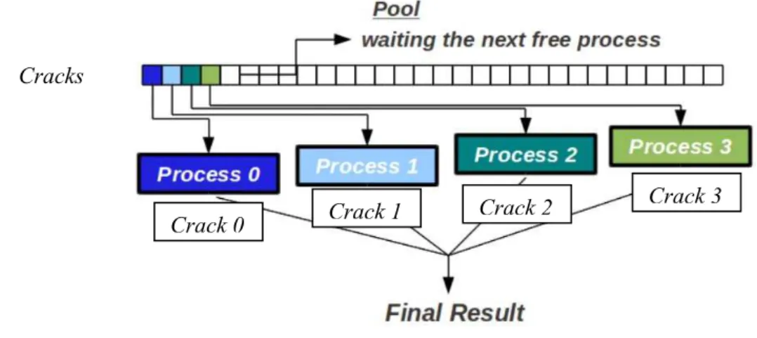
Figure 4.16 Relation between process and cracks (Adapted from Piedade Neto et al, 2011) 96 Figure 5.1 Clouds ωj in R2(Extracted of Barros, 2002) ... 97
Figure 5.2 Partition of Unit from FE in R1(Extracted of Barros, 2002) ... 100
Figure 5.3 Enrichment of the PUM(Extracted from Barros, 2002)... 101
Figure 6.1 Example 1 – Geometry and mesh used in ... 103
Figure 6.2 Example 1 – Fields of interest of the ... 104
Figure 6.3 Example 1 - Local problem and the generated mesh ... 105
Figure 6.4 Example 1 - Stress and displacements fields in the Local problem 106 Figure 6.5 Example 1 – Effects of the enrichment ahead the crack tip ... 107
Figure 6.6 Example 1 – Stress component ahead the crack tip, without the enrichment 107 Figure 6.7 Example 1 - Effects of the enrichment x analytic curves ... 108
Figure 6.8 Example 1 - Analysis of the local problem using Franc-2D® ... 108
Figure 6.9 Example 1 - Mesh of generated by SCIEnCE ... 110
Figure 6.10 Example 1 - Fields of interest of ... 111
Figure 6.11 Example 1 - Propagation of the crack ... 113
Figure 6.13 Example 1 - Fatigue crack growth curve ... 117
Figure 6.14 Example 2 - Three parallel cracks (extracted from Dong and Atluri, 2013) 117 Figure 6.15 Example 2 - Used mesh and displacement fields ... 118
Figure 6.16 Example 2 - Adopted mesh and stress component yy ... 119
Figure 6.17 Example 2 - Propagation of the three parallel cracks in 9 steps ... 119
Figure 6.18 Example 2 - Propagation of the three parallel cracks after 9 steps . 120 Figure 6.19 Example 2 - Propagation of the three parallel cracks after 9 steps . 121 Figure 6.20 Example 3 - An Embedded Slanted Crack ... 122
Figure 6.21 Example 3 - Used mesh and some fields of interest ... 122
Figure 6.22 Example 3 - Propagation of the crack in 5 steps ... 123
Figure 6.22 (continued) Example 3 - Propagation of the crack in 5 steps ... 124
Figure 6.23 Example 4: Domain with embedded slanted crack and hole with crack 125 Figure 6.24 Example 4:Adopted meshes and stress fields of interest ... 126
Figure 6.25 Example 4: SIFs obtained using Franc2D x SCIEnCE (Splitting Method) 127 Figure 6.26 Example 4 - Plate subjected to a tensile load, with 36 holes, and a given pattern of cracks (Andersson & Babuska, 2005) ... 128
Figure 6.27 Example 4 - Model of ... 129
Figure 6.28 Example 4 - (cracks 2, 6, 5, 9, 12) ... 130
Figure A.1 Crack of length equal to 2a, embedded in a remotely loaded plate (Source: Wang, 1996) ... 146
List of symbols
: Vector containing the “ ” parameters ai: Length of the crack i
: Number of the element
C: Constant depending on the material in the fatigue analysis
: Space of functions that, together with all theirs partial derivatives, are continuous and have compact support on
da/dn: Fatigue Crack Growth Rate : Second order stress tensor
: Jump in the traction vector applied in Г contour : Jump in the displacement vector applied in Г contour ΔK: Variation of the Stress Intensity Factor
: Real shape function defined in
: Set of linearly function that generates the enrichment space
, : Set of functions that provides the HP-Clouds
E: Young’s modulus
EPFM: Elastic-Plastic Fracture Mechanics
Г : Rectangular contour of the local sub-problem G: Energy release rate
: General Influence Matrix
GFEM: Generalized Finite Element Method
J: J Integral
: Kolosov constant
Lji: Function in
Lα: Enrichment functions space
m: Constant depending on the material in the fatigue analysis n: Number of cycles in fatigue analysis
Nj(x): Shape function
: Poisson’s ratio
KI, KII, KIII: Stress Intensity Factor, referred to Modes I, II and III, respectively
PK: Basis of the approximation function
: Global sub-problem, similar to the original problem, but without the cracks
: Global sub-problem of the Splitting Method : Local sub-problem of the Splitting Method ( i, i): Coordinate system used to analyze cracks
: Vector containing the weighted tractions in the crack lines in the global problem
R: Energy required per increment of crack extension Rn: Euclidean vector space of dimension n
: Radius of the plastic zone in the plane stress state S: Contour line of the domain V
: Contour of the local domain in the local sub-problem Sci: Contour line of the crack i
: “Positive” crack surface of the crack i : “Negative” crack surface of the crack i Sj: Contour line of the hole j
SIF: Stress Intensity Factor
S : Obtained functions by the multiply of the by the PU in the element Su: Contour where the displacements are imposed
St: Contour where the tractions are imposed
T: Traction vector : Total traction vector
: Traction vector applied in : Traction vector applied in
: Imposed displacement field
ũ : Approximation function
: Displacement field in the Г contour
, : Displacement fields in the x and y directions, respectively
, : Decomposition of the displacements fields in directions 1 and 2, respectively, referred to Mode I
, : Decomposition of the displacements fields in directions 1 and 2, respectively, referred to Mode II
V: Domain of the sub-problems : Local domain containing the crack i
W: Strain energy density
We(xi): Weight function evaluated in xi
XFEM: Extended Finite Element Method
xj: Point in Ω
List of Tables
Table 2.1 ΔKI,eq x a (for a fixed crack) ... 59
Table 6.1 Example 1 – Number of assembled problems to solve example 1 using Splitting Method ... 102 Table 6.2 Example 1 - SIFs obtained from SCIEnCE (GFEM) and Franc-2D®
(FEM) 109
Table 6.3 Example 1 - Error between SIFs obtained from SCIEnCE and Franc-2D® (left crack tip) ... 109
Table 6.4 Example 1 - SIFs obtained from Franc-2D® using different methods
110
Table 6.5 Example 1 - Comparison with analytic solution ... 112 Table 6.6 Example 1 - Values of KIfor a sequence of “half-lengths” ... 114
Table 6.7 Example 3 - KI: Stazi et al x SCIEnCE (Splitting Method) ... 124
Table 6.8 SIFs obtained using Franc2D®et al x SCIEnCE (Splitting Method)
127
Table 6.9 Example 4 - Data for analysis ... 128 Table 6.10 Example 4 - Values obtained by Andersson & Babuska (2005) x
SCIEnCE 130
Table 6.11 Example 4 - KI,max and the respective pattern of cracks ... 131
Nomenclature
COD: Crack Opening Displacement CSD: Crack Sliding Displacement CST: Constant Strain Triangle FEM: Finite Element Method
GFEM: Generalized Finite Element Method LSM: Least Square Method
LST: Linear Strain Triangle PUM: Partition of Unit Method
SGBEM: Symmetric Galerkin Boundary Element Method XFEM: Extended Finite Element Method
Index
Chapter 1: Introduction ... 31 Chapter 2: Fracture Mechanics Topics ... 36 2.1 Opening modes. ... 36 2.2 Stress Functions. ... 37 2.3 On the use of the Generalized Finite Element Method. ... 39 2.4 J Integral ... 42 2.5 “Crack Open Displacement” (COD) and “Crack Sliding Displacement” (CSD) ... 50 2.6 The maximum principal stress criterion. ... 51 2.7 Fatigue Crack Growth. ... 53 2.8 Slow Stable Crack Growth and the R‐Curve ... 60 Chapter 3: The splitting method as a tool for analysis of problems of the Linear-Elastic Fracture Mechanics ... 61
3.1 Introduction ... 61 3.2 The Bueckner principle and superposition models ... 61 3.3 The Splitting Method ... 62 3.4 The global sub‐problem ... 63 3.5 Local Sub‐problem ... 65 3.6 The Global Sub‐problem ... 67 3.7 Assemblage of the problems. Coefficients provided by and ... 69 3.8 Additional features of sub‐problems. ... 70 3.9 Assemblage of the Г contour ... 72 3.10 On the inner product character of the weak form of traction vector nullity
condition. ... 72 3.11 Assemblage of the linear system on the “α” coefficients considering multiple cracks. 74
Chapter 6: Numerical examples ... 102 6.1 Example 1: An Embedded Through‐Thickness Crack ... 102 6.2 Example 2: Three Embedded Parallel Cracks ... 117 6.3 Example 3: An Embedded Slanted Crack ... 121 6.4 Example 4: Plate subjected to a tensile load with a slanted crack and a crack
associated to a hole ... 125 6.5 Example 5: Plate subjected to a tensile load with several cracks attached to holes 128
Chapter 1: Introduction
It is well known that strength failures can be either of the yielding-dominant or fracture-dominant types. Defects are important for both types of failure, but those of primary importance to fracture differ remarkably from those influencing yielding.
For fracture-dominant failures, i.e. fracture before complete yielding of the net section, the size scale of the defects which are of major significance is essentially macroscopic. In other words, the defects can be visualized and, in some circumstances, can be measured. Therefore, it is of great interest to model the effects of cracks on the behavior of solids to more precisely simulate the failure.
The commonly accepted first successful analysis of a fracture-dominant problem was that of Griffith in 1920. Quoting the words of Janssen et al (2006):
“Griffith formulated the now well-known concept that an existing crack will propagate if thereby the total energy of the system is lowered, and he assumed that there is a simple energy balance, consisting of a decrease in elastic strain energy within the stressed body as the crack extends, counteracted by the energy needed to create the new surfaces.”
In the middle of 1950 decade Irwin contributed with another major advance by showing that the energy approach is equivalent to a stress intensity factor (K) approach, according to which fracture occurs when a critical stress distribution ahead of the crack tip is reached. Since then, several methods have been developed to allow evaluating the stress intensity factors in order to offer a description of the crack growth.
Further confirming the importance of fracture mechanics, back to the nineteenth century, the Industrial Revolution led to an enormous increase in the use of metals (mainly irons and steels). Unfortunately, many accidents owing to failure of these structures started to occur. Some of these accidents were due to poor design, but it was also gradually discovered that material deficiencies in the form of pre-existing flaws could initiate cracks and fracture.
Figure 1.1 Liberty ship
(Source: http://inspecaoequipto.blogspost.com.br/2013_11_01_archive.html Researched in 05/01/2015)
The aircraft accident of the Boeing 737-200, which occurred near Maui, Hawaii, in April 28, 1988, is another important example, closer to the field of interest of this work. According to the Official Accident Report, the Failure of the Aloha Airlines maintenance program detected the presence of significant disbanding and fatigue damage which led to failure of the lap joint and the separation of the fuselage upper lobe.
Figure 1.2 Aircraft accident of the Aloha Boeing 737
On the other hand, the analysis of structures of complex geometry, for example, demands the development and employment of robust numerical methods. Moreover, achieve accurate estimates to the stress fields close to the crack tips can be a challenging task, often requiring high cost computational work. In this study, the Generalized Finite Element Method (GFEM) (Duarte et al, 2000; Duarte; Kim, 2008) is explored in face of its known efficacy in the analysis of the linear elastic fracture mechanics problems. In short, GFEM consists of a Partition of Unity Method (PUM) “enriched” with a special class of functions, in which the partition of unity is provided by the shape functions of conventional finite element method.
Even if a good numerical tool is available for the analysis of a cracked solid, in many engineering problems there is a need to analyze the effect of different local crack scenarios in the same structure. For example, recent aircraft accidents have strongly appointed to the need for considering combined effects of multiple growing cracks where each individual crack can be harmless, but the combined effect caused by several cracks can be disastrous. Hence, often it is necessary to consider many possible damage locations and damage sizes in the structures. Obviously, find out the worst scenario can demand an excessive computational effort.
In order to reach this goal, the so called decomposition methods started to be developed. Quoting Alves (2010), Lachenbruch (1961) was pioneered in the use of the Schwartz-Newmann Alternating Method to analyze Fracture Mechanics problems. Such method deals with the Superposition Principle, and the final result is obtained by summation of the solution of two different problems. The first one presents an infinite body containing a crack and aims to capture the local singularity of the problem. The second one refers to a finite domain without cracks. The regular parcel of the solution is obtained of this last problem.
In the sequel, in the work of Nishioka and Atluri (1983), the Finite Element Method was used with analytical solutions of the Alternating Method. However, the calculus of the Stress Intensity Factors was done by an iterative process. As an alternative, Babuška and Andersson (2005) developed the Splitting Method, which consists of a direct method to solve problems containing multiple cracks, therefore avoiding iterative procedures.
solutions for different crack sizes and crack patterns are needed. Aiming a further contribution to the original formulation of the method, a new improved version including mixed mode crack opening effects and aiming the analysis of fatigue by a propagation method is hereby proposed. In this manner, it is possible to realize a deterministic rupture analysis including fatigue and multi-site damage not considered in the early works on the method.
The Splitting Method was implemented in a pre-existent toolkit for the Generalized Finite Element Method program. The SCIEnCE (São Carlos Integrity Environment Computational Engineer) explores the object oriented programming methodology, being its class structure originally conceived by the research group of the Structural Engineering Department of the School of Engineering of São Carlos. More details about the code can be found in Piedade Neto (2013).
Structure of the thesis
As an overall comment, it was the intention of the author to provide a text as concise as possible about the new proposed developments and applications of the Splitting Method, also emphasizing the main features of the developed computational framework. In Chapter 2, the Stress Functions are presented, since they constitute the basis of the enrichment strategy used in GFEM. In addition, concepts like COD, CSD and J Integral are explained because they were implemented in the computational code. Finally, some comments about fatigue crack growth are presented.
Chapter 3 is devoted to the description of the Splitting Method. The mathematical aspects are omitted; however related references are indicated to fulfill this gap.
In Chapter 4, some computational aspects related to the implementation of the Splitting Method are commented either to evidence the difficulties in programming the Splitting Method or to make clear the possibilities for future improvements.
In Chapter 5, a brief review about GFEM is presented, since this strategy was used to reach better accuracy in the numerical results.
Chapter 2: Fracture Mechanics Topics
When modeling multi-cracked solids it is important to have in mind the necessity for answering the following questions, proposed by Broek (1986):
1. What is the residual strength as a function of crack size?
2. What is the maximum size of a crack than can be tolerated at the expected service load; i.e. what is the critical crack size?
3. How long does it take for a crack to grow from a certain initial size to the critical size?
Moreover, the approach hereby adopted also allows addressing the following question:
4. Given many patterns of possible cracks, is it possible to detect the most critical one?
In order to answer properly these questions, firstly some of the main concepts of the Fracture Mechanics of interest must be reviewed. Next, an explanation of how those concepts are used in this research is presented.
2.1 Opening modes.
The “opening modes” are concepts of major significance in Fracture Mechanics and, from now on, they will be claimed along all the work. It is important to mention that there are three independent movements between the crack surfaces, shown in Figure 2.1.
Modes of crack surface displacements (Figure extracted of JANSEEN,
Mode I or “Opening Mode”: the relative movement between the crack surfaces occurs in the perpendicular direction to the plane of the crack;
Mode II or “Sliding Mode”: the displacement of the crack surfaces is in the plane of the crack and in direction perpendicular to the leading edge of the crack;
Mode III or “Tearing Mode”: relative sliding between the crack surfaces caused by out-of-plane shear.
In this work, as the modeling is restricted to two-dimensional analysis, only the Modes I and II are considered.
2.2 Stress Functions.
The Elastic Fracture Mechanics encompasses problems consisting of elastic solids with cracks. An important feature is that, at the crack tips, a singular stress concentration occurs.
The Westergaard (1939) complex stress functions provide the analytical solutions to the fracture mechanics problems. In order to present a brief review of these functions, let be considered an infinite two-dimensional domain containing a crack of length equal to 2a, as shown in Figure 2.2-a. The plate is bi-axially loaded in tension by a stress ∞. According to Janssen et al (2006), the boundary conditions for this problem are:
a. Bi-axially loaded plate (repeated in Appendix A)
b. Local coordinate system
Stress element close to the crack tip and local coordinate system
x y
r
y
ii. x→ ∞and y→ ∞ for x → ±∞ and/or y → ±∞;
iii. y→∞ for x = ±a and y = 0.
Actually, the condition (iii) is a characteristic of the fracture mechanics problems and is obtained from the analysis. However, since it is necessary to find out a complex function that encompasses this condition, it can be stated as a boundary condition.
As detailed in Appendix A, a complex Airy stress function that fulfills the above boundary conditions is:
√ (2.1)
where z = x + iy. The Cartesian axes are placed with origin at the crack tip as shown in Figure 2.2-b.
To the purpose of this section, it is sufficient to know the solutions to the displacements and stress fields in the neighborhood of the crack tip with respect to each fracture opening mode. As already mentioned, more details are given in Appendix A.
Related to Mode I, the components of the solution to the displacements fields are given by:
(2.2)
(2.3)
And, for stress fields:
√ (2.4)
√ (2.5)
√ (2.6)
lim→ √ , (2.7)
The variables r and are the polar coordinates, presented in Figure 2.2-b. In addition, in correspondence to the Mode II, the components are given by:
(2.8)
(2.9)
And for stress fields:
√ (2.10)
√
(2.11)
√
(2.12)
The Stress Intensity Factor (SIF), in equations (2.8)-(2.12), is given by:
lim→ √ , (2.13)
The constant κ appearing in the previous relations for the displacement fields is the Kolosov constant and it can assume the following values:
, for Plane Strain; ⁄ , for Plane Stress.
It is immediate to verify that the stress components tend to infinity at the crack tip (r=0), i.e.:
lim→ ∞; lim
→ ∞ ; lim→ ∞ (2.14)
At this point, it is enough to address directly to the use of Generalized Finite Element Method, from now on called GFEM. More details about GFEM, not necessary to the aim of this section, are given in Chapter 5.
The main feature of the GFEM consists of the “enrichment” of the nodes of the elements that are completely or partially cut by a crack. The enrichment is advantageous when using appropriate functions to capture the displacement fields and the high stress gradients. Taking this into account, the stress functions provided from classical analysis of Fracture Mechanics are adequate to be used as enrichments.
The enriched element shape functions space can be spanned from the following enrichment basis functions:
To elucidate the enrichment effects, the example depicted in Figure 2.3 is presented. This example consists of a plate subjected to a constant traction load, containing a crack on the right edge.
Rectangular plate subjected to a constant load
y x
x = 0
x = 0.75
x = 1.0
x = 2.0
} sin 2 cos , sin 2 sin , 2 sin , 2 cos , 1 {
r r r r
Data of the problem, adopted without units for convenience:
i. Young’s modulus (E) = 1.0; ii. Poisson’s ratio ( ) = 0.3; iii. Traction load (σ) = 1.0; iv. Length of the crack (a) = 1.0.
The plate was discretized using a single quadrilateral finite element. Figures 2.4 and 2.5 depict the enrichment effects, considering several lines positioned along the x-axis.
Stress field yy
-4 -3 -2 -1 0 1 2 3 4 5 6
00 02 04 06 08 10 12 14 16 18 20
S
tr
ess F
ie
ld
σ
yy
y-coordinate (Figure 2.3)
Displacement field uy
It is possible to note in Figure 2.4 that the stress component yy tends to infinity at
crack tip (x = 0.9999…) and there was a discontinuity in the displacement component uy
for x < 1.0.
This example is very simple but shows the effectiveness of the enrichment in the modeling of the phenomenon that occurs in the neighborhood of the crack tip. Use of the GFEM combined with the refinement of the mesh must provide better results.
2.4 J Integral
Aiming to evaluate the Stress Intensity Factors (SIFs), Rice (1968) formulated the J Integral concept. It addresses a path-independent line integral which value has correspondence to the decreasing in potential energy when an increment of crack extension occurs. The J Integral applies either in linear or nonlinear elastic materials.
Moreover, an important advantage of the J Integral, quoting Broek (1986) is that “within certain limitations, the J Integral provides a means to determine an energy release rate for cases where plasticity effects are not negligible”. This characteristic of the J Integral is important in order to guarantee that the Splitting Method can be extended do analyze problems involving ductile materials. However, this aspect was not considered in this work. -12 -11 -10 -9 -8 -7 -6 -5 -4 -3 -2 -1 0 1 2 3 4 5 6 7 8 9 10 11 12
0 2 4 6 8 10 12 14 16 18 20
D is p la cem ente co m p o n ent dy
y-coordinate (Figure 2.3)
The J Integral can be represented by:
∙
Г (2.22)
or, in an alternative expression, conveniently using indicial notation, as:
n ∙
Г (2.23)
where:
i. W is the strain energy density:
, (2.24)
ii. The traction vector T is a force per unit area acting at a point with respect to a plane defined by a normal versor n, as shown in Figure 2.6.
(2.25)
Arbitrary path Г enclosing a crack tip. Traction vector T and
normal vector n to the segment ds
It is important to verify in Figure 2.6 that the path of integration Г is not, necessarily, circular. However, in this work a circular path was adopted in order to take advantage of some favorable features of the polar coordinates. Therefore:
x y
o
ds
cos (2.26)
The J Integral can be viewed as an energy parameter, comparable to the energy release rate G, or else, G=J, in the elasticity limit. Finally, it is important to remind the relations between J Integral and the Stress Intensity Factors:
(Plane Stress) (2.27a)
(Plane Strain) (2.27b)
To evaluate the J Integral numerically, a particular procedure is hereby proposed. First of all, let be a circular path of integration around the crack tip. This path is divided into 4 segments. Next, each segment is further subdivided into 3 segments. Therefore, there are 4 segments, each one with 2 intermediate points. The reason is due to the option of mapping an arc of circumference through a polynomial of order 3. In Figure 2.7a, the referred segments can be observed: i) 0-1-2-3; ii) 3-4-5-6; iii) 6-7-8-9; iv) 9-10-11-12.
Remark: The finite element mesh adopted to discretize the neighborhood of the crack tip is omitted to focus only the integration path. The axes depicted in the figure are local axes.
a. Circular path subdivided into segments b. Natural coordinates
Path of integration
In the next step, the integration along the path Г must be done using each discretized segment. In other words, the integration along Гis substituted by a sum of integrals along each segment, as shown in Equation 2.28:
∙ n ∙
Г ∑ Г ∙ n ∙ (2.28)
where nseg is the number of segments in which the path Г is divided. In the example shown in Figure 2.7a, nseg is equal to 4.
Afterwards, each integral on the right hand side of Equation (2.28) is made using the natural coordinate system defined above and shown in Figure 2.7-b:
∙ n ∙
Г ∙ n ∙
.
. . , . . (2.29)
where Jac is the Jacobian operator relating the natural coordinates to the local coordinates.
The relation between natural coordinates and local coordinates is well known and given by:
(2.30a)
(2.30b) where:
/ (2.31a)
/ (2.31b)
/ (2.31c)
/ (2.31d)
Finally:
/
Finally, the right hand side of Equation (2.28) can be substituted by a numerical integration:
∙ n ∙
.
. . ∑ ∙ .
(2.33) where:
1. ngp is the number of sampling points of the Gauss quadrature; 2. xi is the ith sampling point;
3. We(xi) is the weight function evaluated in xi.
The sampling points of the Gauss quadrature ngp coincide with the points shown in Figure 2.7-b. In order to calculate Equation (2.33), the required displacements and stress fields must be obtained only at the points shown in Figure 2.7-a, owing to the correspondence between them and the points of the mapping shown in Figure 2.7-b. Both fields can be obtained by using the procedures described in Section 4.1 and Appendix B. However, instead of computing Equation (2.33) directly, it is necessary to divide J in order to obtain KI and KII separately. This procedure was presented by Ishikawa et al
(1980) and used by Kzam (2009). According to Equation (2.34), the J Integral can be separated into two parts:
J = JI + JII (2.34)
where:
1. JI refers to Mode I of opening;
2. JII refers to Mode II of sliding.
To calculate JI, the displacements and stress fields are replaced by auxiliary fields
uI and I, respectively, according to Equations (2.35) and (2.36):
(2.36)
In Equation (2.35), , is the displacement field at a symmetric point of the point that is been analyzed in relation to the local x-axis. Similarly, in Equation (2.36) , is the stress field at the same point. For example, in Figure 2.7a, the point “12” is the symmetric of point “0”, point “11” is the symmetric of point “1” and so on. Obviously, the reciprocal is also true.
Furthermore, to evaluate JII, the auxiliary fields are given by:
(2.37)
(2.38)
In Figure 2.8, the results of the operations correspondent to Equations (2.35)-(2.38) are presented for an arbitrary point P and its symmetrical point P’.
Mode II
Symmetric and anti-symmetric components of the displacement
field for Modes I and II
Analyzing Equations (2.35)-(2.38), and by observing Figure 2.8, it can be calculated that for Mode I:
i. , , ´
ii. , , ´
iii. , , ´
iv. , , ´
v. , , ´
And, for Mode II:
vi. , , ´
vii. , , ´
x y o 11,P I 22,P I 12,P I 22,P' I 12,P' I 11,P' I P P' x y o
u1, P
I
u2, P
I
P
P'
u1, P' I
u2, P' I x y o 11,P II 22,P II 12,P II P 22,P' II 12,P' II 11,P' II P' x y o
u1, P
II
u2, P
II
P
P' u2, P'
II
u1, P
viii. , , ´
ix. , , ´
x. , , ´
An important aspect that must be mentioned is that loads are applied to the crack surfaces and their contributions must be considered in the calculus of the J Integral. To address this issue, the solution proposed by Karlsson and Bäcklund (1978), was hereby adopted. Accordingly, a decomposition of the J integral is assumed as:
J = Jcp + Jscs + Jics (2.39)
where Jcp is the contribution of the circular path to the J Integral and Jscs , Jics are the
contributions of the superior and inferior crack surfaces, respectively.
The procedure to compute the values of Jscs and Jics is identical to that described
above for the calculus of the J Integral in the circular path, and each crack surface is analogously divided into 3 segments and then mapped into a linear segment. See Figure 2.9.
J Integral at the crack surfaces
It is important to observe the direction of the integration indicated by the arrows in the Figure 2.9. The positive outward normal vector n to each crack surface is also indicated.
The procedure to evaluate the contribution of the crack surfaces for the J Integral is identical to that described for the contributions in the circular path. However, it was treated separately in this paper in order to emphasize some important features:
x y
0 1 2 3
0' 1' 2'
n'
1. Most of the programs containing routines for calculating J require a specification of an integration path around the crack tip from the user, assuming that the crack surface is traction free. This is not an assumption in the developed code;
2. The error in the calculus of the J Integral including the crack surfaces can be strongly affected by the accuracy of the stress field very close to the crack tip. Therefore, special care must be taken aiming to improve the accuracy in that region, for example, by refining the mesh or, as hereby adopted, by using enrichment strategies.
2.5 “Crack Open Displacement” (COD) and “Crack Sliding Displacement”
(CSD)
The COD method was hereby considered in order to provide an alternative respecting the J Integral. The extraction of SIFs by means of displacement correlation technics is done using the displacements at the crack surface resulting from the analysis.
∙ ∙ (2.40a)
∙ ∙ (2.40b)
where:
1. COD (“Crack Opening Displacement”) is the difference between the normal displacements in correlated points placed at the crack surfaces. It is recommended, or better, it is usual to place the referred points at a distance between 15% up to 50% of the half-length of the crack;
COD and CSD (Source: Leonel, 2010)
2.6 The maximum principal stress criterion.
The main purpose of this section is to establish a criterion to evaluate the angle in which the crack growth will occur. This topic is worth to addressing, once the computational program developed in this work treats of the fatigue crack growth under mixed mode loading.
The maximum principal stress criterion postulates that crack growth will take place in the direction perpendicular to the maximum principal stress. If a cracked solid is loaded in combined mode I and II, the and r at the crack tip (i.e., when dr tends to zero, see
Figure 2.11) are given by the following expressions:
√ cos sin (2.41)
Stress element rotated in relation to a local system
The stress will be the principal stress if r = 0. This is the case for = c where c is found from equating the Equation (2.42) to zero:
sin cos (2.43)
The Equation (2.43) can be solved by writing:
sin cos (2.44)
which yields:
(2.45)
so that:
, (2.46)
and finally:
x y
dr
r
, atan (2.47a)
, atan (2.47b)
The principal stresses are then given as:
, √ , , , (2.48a)
, √ , , , (2.48b)
If | | | |, then , is used as the propagation angle. In the other hand, if | |
| |, then , is used as the propagation angle.
2.7 Fatigue Crack Growth.
In this section, the description of the Fatigue Crack Growth using the Splitting Method is presented. The possibility of taking into account several patterns of cracks and their respective paths of propagation is indeed an important advancement achieved by this work.
The main aim of this analysis is to determine the so-called Fatigue Crack Growth Rate Curve (da/dn x ΔK) and construct the crack length versus the number of cycles curve (a x n). It is important to stress that:
1. da/dn is the crack length growth with respect to the number of cycles;
2. ΔK is the amplitude of the Stress Intensity Factor. In fact, ΔK is a function of a and , or else, ∆ , .
and a crack growth law, the aim is to determine the so-called Fatigue Crack Growth Rate Curve by means of an analytic integration.
In order to elucidate these concepts, let’s consider the cracked plate of the Figure 2.12.
Cracked plate (Extracted of JANSEEN, 2002)
In this case, the Stress Intensity Factor related to the Mode I is given by the Equation (2.49):
∙ √ (2.49)
where a is the half-length of the crack. According to Feddersen (1967), Cg is given by
Equation (2.50):
sec (2.50)
It is clear that, for a given crack length, the Stress Intensity Factor depends upon of the level of the applied load. It follows that the amplitude of the Stress Intensity Factor is directly related to the amplitude of the applied load. Thus, the Equation (2.49) becomes:
In Figure 2.13 a possible variation of an applied cyclic load is exemplified.
Level of the tensile load x time
For an arbitrary, but fixed, crack length 2a, there is a maximum Stress Intensity Factor KI,max associated to max and a minimum Stress Intensity Factor KI,min associated to
min. Therefore, the amplitude of the Stress Intensity Factor is calculated as follows:
∆ , , (2.52)
For the Fatigue Crack Growth Rate Curve da/dn x ΔK, in this work it is adopted the most widely known crack growth law, the Paris equation:
∆ (2.53)
where C and m are constants depending on the material.
Once integrating the Equation (2.53), it is possible to construct a crack length versus
time
x time
σmax
∙ ∆ √ (2.54)
Integrating the Equation (2.54), the crack length versus the number of cycles curve (a x n) arises. However, many structures are not only subjected to pure tension but they can be subjected to shear and torsional loading. Cracks may therefore be exposed to tension and shear, which leads to mixed-mode crack opening, i.e., a mixture of modes I and II. In order to taking in account the mixed mode fracture, ΔKI must be replace by
ΔKI,eq in Equation (2.53), which is determined as follows:
, ∙ cos ∙ ∙ cos ∙ sin (2.55a)
and, consequently:
∆ , ∆ ∙ cos ∙ ∆ ∙ cos ∙ sin (2.55b)
where c is the direction of crack growth, defined in Section 2.6. For more details about
Equations (2.55a) and (2.55b), see Broek (1986).
For a few problems it is possible to find relations such as (2.49) and (2.51), which are closed forms that can be integrated analytically. Nevertheless, for more complex problems, presenting complex geometry, loading and patterns of cracks, such relations are not available. A possible manner to solve this problem is to determine the amplitude of the Stress Intensity Factors versus the crack length curve using discrete values of the crack lengths and calculating theirs respective SIFs using the Splitting Method, which has provide good numerical estimates for the Stress Intensity Factors.
A simple methodology based on the Splitting Method is hereby proposed for solving problems with many cracks in order to determine each singular crack growth law and evaluate the fatigue crack growth rate.
The main steps of the conceived procedure are described in the sequel:
1. Choose a suitable increment of crack growth Δamax, which must be small enough
2. By using the Splitting Method, calculate the Stress Intensity Factors KI and KII
for each crack tip, considering theirs original lengths. By using the Equations (2.55a) and (2.55b), calculate ΔKI,eq. Comparing the whole set of values,
determine the maximum value of ΔKI,eq, from now on indicated as ΔKI,eq. max.
Therefore;
∆ , . ∆ , , . . (2.56)
Remark: for internal cracks, there will be more than one tip for each crack.
3. The crack length increments are defined as suggested by Sing et al (2012), “for multiple crack problems, first a principal crack tip is decided on the basis of maximum value of ΔKI,eq, then a constant value of maximum crack (Δamax) can
be taken for this principal crack tip”. Then, the remaining crack increments are obtained as:
∆ ∆ ∙ ∆ , ,
∆ , . j = 1...number of crack tips (2.57)
where m is the exponent of the Paris Law, see Equation (2.53).
4. The previous steps must be repeated over the required number of steps, previously established in the analysis. Each crack must be increased according to Equation (2.57). For example, in the first iteration, for an arbitrary crack tip j, the length will be:
aj,1 = aj,0 + Δaj (2.58)
where:
i. aj,1 is the half-length of the crack tip j in the first iteration;
ii. aj,0 is the half-length of the crack tip j in the original configuration;
iii. Δaj is the increment calculated using the Equation (2.57).
In Figure 2.14, a graph relating KI,eq and the half-length a of an arbitrary crack is
( min). It is possible to verify from the graph that discrete values are presented and each
pair of values is related to a fixed crack length. An example is shown in Figure 2.15.
KI,eq x a for an arbitrary crack
Using the values of KI,eq related to max and min, it is possible to evaluate ΔKI,eq:
∆ , , , , , (2.59a)
Obviously:
, , , ∙ cos ∙ , ∙ cos ∙ sin
, , , ∙ cos ∙ , ∙ cos ∙ sin
(2.55a – repeated)
After solving the problem using this procedure for a considerable number of steps, it is possible to construct a table relating ΔKI,eqand a for each crack, by using Equation
(2.55b):
KI,eq
a (half crack length)
ΔKI,eq
σmax
σmin
Table 2.1 ΔKI,eq x a (for a fixed crack)
a a0 (original
crack)
a1 a2 … anstep
ΔKI,eq ΔKI,eq, 0 ΔKI,eq, 1 ΔKI,eq, 2 … ΔKI,eq, nstep
Next, a polynomial approximation function of degree p can be constructed from the obtained values by means of the LSM.
∆ , ≅ ∙ ∙ ∙ (2.60)
Remark: in fact, the Equation (2.60) is a function that depends only on the crack length a for an arbitrary, but fixed, Δ . However, it is feasible to construct an approximation function in which Δ be a function of a or the number of cycles n.
The polynomial approximation function of ΔKI,eq is shown in Figure 2.15.
ΔKI,eq x a for an arbitrary crack
Substituting (2.60) in (2.53) and integrating, it is possible to recover the relation between the length of the crack (a) and the number of cycles of alternating stress (n).
The presented method is especially useful when the relation between ΔK and a is unknown. In this work, the analysis of a problem containing a closed expression relating ΔK and a was performed aiming to validate the procedure and is presented further on in
ΔKI,eq
2.8 Slow Stable Crack Growth and the R-Curve
To conclude the review of the Fracture Mechanics topics, the author deems be necessary to establish a criterion to assess the crack resistance and consequent failure of the analyzed solid. Accomplished with that criterion the proposed method becomes feasible for performing a complete study of a given problem, including the verification of some possibilities of failure.
It is possible to state that there are at least two main reasons that endorse the necessity for establishing a criterion to stop the incremental process used in this work:
1. The proposed method will model the real phenomenon with better accuracy of an engineer view point, since the limit to the crack growth from which the failure follows could be determined;
2. If a criterion to stop the incremental process is established, it is possible to avoid an excessive number of increments and, consequently, saving computational effort. The time saved in the process could be used to analyze other patterns in other problems with many cracks, for example.
It was already mentioned that, for each crack tip, and for each step of the analysis described in the Section 2.7, the method will provide the Stress Intensity Factors KI and
KII. To assess if the crack growth will be unstable, one can to apply the Equation (2.61)
using the referred SIFs (BROEK, 1986):
(2.61)
where KIc and KIIc is the critical Stress Intensity Factor referred to the opening Modes I
and II, respectively, and are material properties.
In many cases, KIc = KIIc. In these cases, it is possible to apply the Equation (2.62):
Chapter 3: The splitting method as a tool for analysis of problems
of the Linear-Elastic Fracture Mechanics
3.1 Introduction
The superposition technic is probably the most common technic for obtaining the SIFs. In this chapter it is shown how such technic is explored in the Splitting Method in order to solve two-dimensional problems of solids presenting internal and external cracks, as well as cracks linked to the borders of holes.
3.2 The Bueckner principle and superposition models
Bueckner (1958) stated that “[a]ny crack or notch problem can be reduced to one where the external load appears in the form of tractions distributed over the faces of the crack.” This is called the Bueckner’s principle, illustrated in Figure 3.1.
Figure 3.1 Bueckner principle
In addition, according to Janssen (2006), “in the vicinity of the crack tip the total stress field due to two or more different mode I loading systems can be obtained by an algebraic summation of the respective stress intensity factors.” This is the superposition principle.
3.3 The Splitting Method
The Splitting Method belongs to the class of decomposition methods and was originally proposed by Andersson & Babuska (2005). In this section, the main concepts of the method are addressed. Complementary aspects can be found in Alves (2010).
Figure 3.2 illustrates the problem to be analyzed using the Splitting Method. The two-dimensional linear elastic domain Vc has a boundary S divided into two
non-intersecting complementary parts Su and St (S = St U Su and St ∩ Su = ø) on which
restrictions over displacements and loading can be prescribed, respectively. The domain contains holes with cracks, an internal crack and a border crack and is submitted in its boundary St to a tensile load.
Figure 3.2 Two-dimensional domain containing holes and cracks.
Assuming that in Su the displacement vector u is prescribed, the equations
governing the equilibrium conditions and the static boundary conditions of the problem are:
∆ on Vc (3.1a)
⁄ on St (3.1b)
⁄ on Sci, i = 1…4 (3.1c)
where Δ(.) is the ‘generalized’ Laplacian operator. In fact, the first condition is a condensed form of representing Lamé’s equations, in which also the geometrical characteristics of deformations and the elastic properties of the material are implicit. Equation (3.1b) is a boundary condition making the stress tensor T and the applied loading compatible. In particular, Equation (3.1c) means that the crack surfaces are traction free.
n
internal crack border crack
hole border crack
S Sc1
S1 a1
S S3
u = 0
n
internal crack border crack
hole border crack
S Sc1
S1 a1
S S3
u = 0
In the Splitting Method the above problem is divided into sub-problems. The basic aim is to find a stress vector solution t at the crack faces such that:
(3.2)
where and are stress vector solutions at the crack lines obtained from the sub-problems and , respectively, and is the stress vector prescribed at the crack faces in the local sub-problem .
In Alves (2010), the numerical performance of the Splitting Method was improved by combining it with enrichment strategies of the approximation functions.
The main aim of the present research is to extend the scope of the Splitting Method to assess fatigue problems, by incorporating a step-by-step crack propagation procedure. An additional important improvement included in the extended scope is the possibility of evaluating SIFs for I-II mixed mode.
According to the theoretical conception of the method, it is possible to consider border cracks, holes with cracks and internal cracks. However, in the computational code developed in this work, only holes with cracks and internal cracks were considered.
This chapter is mostly devoted to describe the sub-problems composing the method. Each sub-problem will be described in detail in the sequel.
3.4 The global sub-problem
The global sub-problem is basically the original problem without the cracks. However, identification lines are placed where should be the center lines of the original cracks. From the analysis of the , traction vectors will be identified in those lines.
Thus, the governing equations of this type of sub-problem are:
∆ on V (3.3)
⁄ on St (3.4)
where V is the domain of the un-cracked domain and is the displacement field related to it.
Therefore, it is also important to highlight the following geometric features and variables:
3. Identification line Sci of the crack i. In fact, this line is not modeled, but it
must be considered in order to evaluate the traction vector;
4. Boundary line Sj of the hole j. It is possible to solve problems with different
numbers of cracks and holes (see Figure 3.2);
5. Local coordinate system ( i, i). The i-axis must be aligned with the crack ai.
The origin of the local system must be placed at crack tip, as depicted in Figure 3.2;
6. Length of the crack: ai.
It is also important to mention:
i. Segment Su of the boundary line S where displacement components are
prescribed:
on Su; (3.5)
ii. Complementary segment St of the boundary line where traction vector is
imposed:
⁄ . ̅ on St; (3.6)
Obviously, S =St U Suand St∩ Su =
ø
.iii. Null traction vector along the internal hole boundary Si:
. on Si. (3.7)
Due to the simplicity of this sub-problem, it is possible to use a coarse mesh in the discretization can be defined. In fact, it is adequate to adopt a refinement in the mesh only to ensure some accuracy around the holes and identification lines corresponding to the original cracks. Therefore, local enrichment of the approximation may be exempt, by setting up a situation in which GFEM/ XFEM coincides with FEM.
sub-problem. In fact, as the numerical solution provides components of the traction vector at some arbitrary points along the line Sci, a continuous approximation of these components
can be recovered by means of the Least Square Method (LSM). More specifically, the continuous approximation is written as a linear combination of an adopted polynomial basis function.
3.5 Local Sub-problem
The basic aim of this sub-problem is to compute the SIFs using GFEM/XFEM. By using fracture functions as local enrichments it becomes feasible to consider the effects of the singularities without demanding an excessive mesh refinement.
In each local sub-problem, only one crack is considered. This crack may be an internal crack or a hole with a crack, as depicted in Figure 3.3. Surrounding the crack or the crack and hole, an arbitrary rectangular contour should be made, hereafter represented as Г . It is important to mention that Г cannot intercept other cracks.
In each sub-problem, a set of internal pressure loads is applied to the crack faces, using the same normalized polynomial basis (it means, each component has a maximum unitary value) employed in the global sub-problem to identify the continuous traction vectors along the crack lines. Finally, as well as the SIFs, for each component of the polynomial basis, the displacement field and the traction vector t(i) along Г are
also computed.
Figure 3.3 Local Sub-Problem
The governing equations of this type of sub-problem are:
1. Local domain containing the crack: ; 2. Boundary line of the local domain: ; 3. Line Sci of the crack i;
4. Local coordinate system ( i, i). The origin of the system must be placed at
the crack tip;
5. Length of the crack i: ai;
6. Arbitrary rectangular contour enclosing the hole and the crack i: Г . Moreover, the main features of this type of sub-problem are:
i. Prescribed displacement field in , aiming to avoid rigid body movement of :
on ; (3.9)
Remark: The boundary conditions are arbitrary. The only restriction is that they must avoid the rigid body movement.
ii. Null traction vector at the hole border:
⁄ . on Si; (3.10)
iii. Traction vector applied at the crack surface: the components of this vector are polynomial functions of the natural coordinate i:
⁄ on , (3.11a)
⁄ on . (3.11b)
Where:
⁄ ⁄ , , , (3.12)
It is clear that any approximation function will be represented as a linear combination using elements that belongs to this set.
3.6 The Global Sub-problem
The Global Sub-problem is geometrically similar to . Therefore, geometry is described without cracks as well and the same boundary conditions of the are considered. However, only the displacement field and traction vectors identified in Г of the correspondent local sub-problem are imposed as “jumps” on . It is important to note that the number of global sub-problems coincides with the number of local sub-problems.
It is important to state in this point that represents the solution of the sub-problem and consists of the displacement field in the domain V of the plate.
The governing equations of this type of sub-problem are:
∆ on V (3.13)
⁄ on St (3.14)
The main imposed restrictions to this sub-problem are:
1. Dirichlet boundary conditions, which are the same ones as the sub-problem :
on Su (See also Equation 3.5); (3.15)
2. Newman boundary conditions consisting of null traction vector in St and in
the hole borders:
⁄ on St, (3.16)
⁄ on Si. (3.17)
Finally, it is very important to highlight the “jumps” that must be prescribed: 3. “Jump” in the traction vector on the Г :