www.atmos-chem-phys.org/acp/3/233/
Chemistry
and Physics
Modeling the chemical effects of ship exhaust in the cloud-free
marine boundary layer
R. von Glasow1,3, M. G. Lawrence1, R. Sander1, and P. J. Crutzen1,2
1Max-Planck-Institut f¨ur Chemie, Atmospheric Chemistry Division, PO Box 3060, 55020 Mainz, Germany
2Center for Atmospheric Sciences, Scripps Institution of Oceanography, University of California at San Diego, La Jolla, CA
92093-0221, USA
3now at Scripps
Received: 19 April 2002 – Published in Atmos. Chem. Phys. Discuss.: 7 June 2002 Revised: 31 January 2003 – Accepted: 3 February 2003 – Published: 21 February 2003
Abstract. The chemical evolution of the exhaust plumes of ocean-going ships in the cloud-free marine boundary layer is examined with a box model. Dilution of the ship plume via entrainment of background air was treated as in stud-ies of aircraft emissions and was found to be a very impor-tant process that significantly alters model results. We esti-mated the chemical lifetime (defined as the time when dif-ferences between plume and background air are reduced to 5% or less) of the exhaust plume of a single ship to be 2 days. Increased concentrations of NOx(= NO + NO2) in the
plume air lead to higher catalytical photochemical produc-tion rates of O3and also of OH. Due to increased OH
con-centrations in the plume, the lifetime of many species (espe-cially NOx) is significantly reduced in plume air. The
chem-istry on background aerosols has a significant effect on gas phase chemistry in the ship plume, while partly soluble ship-produced aerosols are computed to only have a very small ef-fect. Soot particles emitted by ships showed no effect on gas phase chemistry. Halogen species that are released from sea salt aerosols are slightly increased in plume air. In the early plume stages, however, the mixing ratio of BrO is decreased because it reacts rapidly with NO. To study the global ef-fects of ship emissions we used a simple upscaling approach which suggested that the parameterization of ship emissions in global chemistry models as a constant source at the sea surface leads to an overestimation of the effects of ship emis-sions on O3of about 50% and on OH of roughly a factor of
2. The differences are mainly caused by a strongly reduced lifetime (compared to background air) of NOx in the early
stages of a ship plume.
Correspondence to:R. von Glasow ([email protected])
1 Introduction
The effects of the emissions of ships on cloud albedo were first described by Conover (1966). In the last decades many more studies dealt with the impact of ship exhaust on cloud albedo and microphysics (e.g. Coakley et al., 1987; Acker-man et al., 1995; Ferek et al., 1998; Durkee et al., 2000b). The impact of ship exhaust on the chemistry of the marine boundary layer (MBL), however, has only recently received attention. Streets et al. (1997) published estimates of SO2
emissions from international shipping in Asian waters and of the contribution of ship emissions to the deposition on land around the Asian waters. The first global compilation of NOxand SO2emissions from ocean-going ships was
pre-sented by Corbett and Fischbeck (1997) and Corbett et al. (1999). They estimated global annual emissions of NOx to
be 10.12 teragram (Tg) per year (3.08 Tg N a−1) and 8.48 Tg of SO2 per year (4.24 Tg S a−1) in 1993. The sulfur
emitted by ships corresponds to roughly 20% of the biogenic dimethylsulfide (DMS) emissions from the oceans. In some regions of the Northern Hemisphere ship emissions can be of the same order of magnitude as model estimates of the flux of DMS whereas they are much smaller than DMS emissions in the Southern Hemisphere. Streets et al. (2000) published updated values for the sulfur emissions in and sulfur depo-sition around Asian waters. They also estimated that ship emissions in the oceans off Asia increased by 5.9% yearly between 1988 and 1995.
be a dominant contributor to SO2concentrations over much
of the world’s ocean and in several coastal regions. Further-more they estimated the global indirect radiative forcing due to ship derived particles to be−0.11 W m−2. In ocean ar-eas with busy ship traffic 30–50% of the predicted non-sea salt sulfate was due to ship emissions and even in the South-ern Hemisphere with very little ship traffic about 5% of the nss-sulfate was predicted to be derived from ship emissions. In another study with a different global chemical transport model Lawrence and Crutzen (1999) investigated the effects of NOx emissions on the budget of O3and OH and found
that in heavily traversed ocean regions the OH burden was predicted to increase up to fivefold. This would reduce the atmospheric lifetimes of reactive trace gases and could have an effect on aerosol particle production and cloud properties as OH is an important oxidant for DMS. O3concentrations
were estimated to increase by a factor of more than 2 over the central North Atlantic and Pacific.
Using an updated emissions inventory and a different global model, Kasibhatla et al. (2000) qualitatively con-firmed the effects predicted by Lawrence and Crutzen (1999), though due to a different geographic distribution of the emis-sions, the effects were more widespread and peak enhance-ments not as large. Comparing the model predictions with results from measurement campaigns they found a difference in NOxof about a factor of 10, therefore showing no support
for the model predicted enhancements of NOx. They
con-cluded that the parameterized description of plume dynamics and/or missing knowledge of the plume chemistry could be the cause for an overestimation of the effects of ship emis-sions.
Davis et al. (2001) used the global model of Kasibhatla et al. (2000) to further examine the issue using data taken over the north Pacific Ocean during five field campaigns over the time period 1991 to 1999. They also found a tendency for this global model including ship emissions to overestimate the observed NOxlevels by a factor of 3.3 during spring and
a factor of 5 during fall. However, even without ships, their simulations overestimate the observed NOxby about 100%,
for unknown reasons (all numbers are from their Table 1). Davis et al. (2001) also proposed a possible reason for the large overestimate with ship emissions. The OH concentra-tion is one of the main factors in determining the NOx
life-time (via reaction with NO2 to form HNO3, which is then
generally deposited). OH concentrations depend strongly on NOx levels. They suggested that in plume air [OH] is high
and therefore the NOxlifetime reduced, resulting in smaller
NOxmixing ratios. This could help explain the tendency for
global models to overestimate the observations because the different plume stages are not resolved in global models.
To yield a better understanding of the chemical processes and the importance of plume dilution we developed a box model to study these processes in detail. With the help of this model, we discuss ship plume chemistry in greater detail than previous studies; in particular we include in a simplistic
way the dilution of a ship plume, which is highly concen-trated directly after emission and subsequently diluted. Our box model includes detailed gas and aerosol phase chem-istry as well as the entrainment of clean background air. We included halogen chemistry (bromine and chlorine released from sea salt aerosol) and emissions of aerosol particles by the ships. In Sect. 2 we describe the model and the treat-ment of the plume expansion. In Sect. 3 we discuss model results of a single plume in detail to point to the most im-portant processes. In Sect. 4 we consider the effects of over-lapping plumes and use an upscaling approach to assess po-tential global effects of ship emissions. Given the scarcity of field measurements and other studies this paper is of ex-ploratory nature rather than trying to find final answers.
2 Model description
The time dependent photochemical box model employed here is based on an updated version of the box model MOCCA by Sander and Crutzen (1996) and Vogt et al. (1996) (the updated set of reactions can be found under http:// www.mpch-mainz.mpg.de/∼sander/mocca). The model con-siders 131 gas phase (H-O-S-C-N-Br-Cl) reactions that are important for the chemistry of the MBL including halogen chemistry. A very comprehensive reaction set with 136 aqueous phase reactions, 11 heterogeneous reactions and 22 equilibria is used for sulfate and sea salt aerosols. We also included 4 irreversible heterogeneous reactions on soot aerosol. The model uses a Gear solver as part of the FAC-SIMILE software (Curtis and Sweetenham, 1987). The pho-tolysis rates are calculated with a four-stream model using the approach of Br¨uhl and Crutzen (1989).
2.1 Mixing of background and plume air
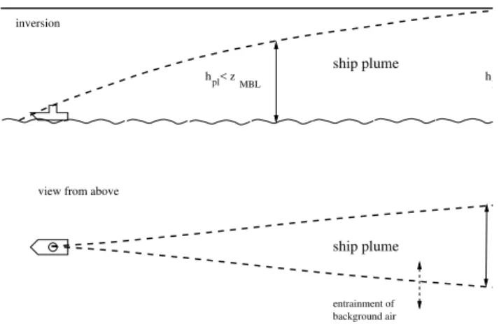
The approach that is used for the mixing of plume and back-ground air has been adopted from studies of the evolution of aircraft exhaust (e.g. K¨archer, 1999). The plume sion in these parameterizations is described with an expan-sion coefficient that has to be determined empirically. In the description of point sources on the surface (e.g. power plant plumes) often Gaussian plume expansion is assumed (e.g. Seinfeld and Pandis, 1998). The parameters needed for the latter approach can be determined from atmospheric stability data with further assumptions on boundary conditions. Our approach is similar to the Gaussian approach with the main difference that in our approach the parameters used for the calculation of the plume expansion do not vary with time. A main restriction of both our and the Gaussian plume expan-sion approach is, that inhomogeneities perpendicular to the direction of ship movement of the plume evolution cannot be accounted for. This restriction can only be overcome with the use of three-dimensional models (e.g. Large Eddy Sim-ulation (LES) models). We did not try to parameterize the in-plume inhomogeneities, but concentrated on the entrain-ment of background air into the ship plume.
For the box model two reservoirs of air are considered: the plume and the background reservoir. Both are assumed to be well-mixed. Dilution of the plume takes place by expan-sion of the plume and associated entrainment of background air. This means that we are effectively running two identi-cal copies of the box model (one for each reservoir of air) at the same time with the same reactions, photolysis rates etc. but that ship emissions are considered only in one reser-voir and that the undisturbed, background reserreser-voir (which remains uninfluenced by the former one) serves only to pro-vide the appropriate background concentrations of gases and particles for the entrainment (one-way coupling). We assume that mixing occurs only perpendicular to the ship’s course (in the vertical and in the horizontal, see Fig. 1). The expansion of the plume can be formulated as:
wpl(t )=w0
t
t0
α
(1)
hpl(t )=h0
t
t0
β
(2)
wherewpl andhpl are the width and height, respectively, of the plume at timet, t0 is a reference time, here chosen to
be 1 s after plume release andw0 andh0are reference
di-mension of the plume at timet0. They were estimated from
data in the literature (see references in Table 1) to be 10 m and 5.5 m, respectively, and correspond approximately to the cross-sectional area of a plume after 1 s. αandβ are the plume expansion rates in the horizontal and vertical, respec-tively.
h < zpl
MBL h = z
ship plume
view from above view from the side
ship plume
inversion
entrainment of background air
pl
Fig. 1.Schematic of the assumed plume expansion. The bold hor-izontal line indicates the inversion that caps the MBL. The dashed lines show the extent of the ship plume.
The change in concentration in the plumecplthrough mix-ing can be written as:
dcpl
dt
mix
=(cbg−cpl) 1
Apl
dApl
dt (3)
with the background concentrationcbgand the cross section of the plumeApl. The plume cross section (semi-ellipse) is given asApl =π/8wplhpl. Using this definition forAplone gets:
1
Apl
dApl
dt =
1 π 8
w0h0 t0αt0βt
α+β π 8w0h0
t0αt0β
(α+β)tα+β−1
= α+β
t
(4)
The top of the MBL is assumed to be impenetrable by the plume, therefore the vertical expansion of the plume stops when hpl reacheszMBL, which is the height of the MBL. Equation 3 can now be written as:
dcpl
dt
mix =
α+β
t (cbg−cpl) hpl(t ) < zMBL α
t(cbg−cpl) hpl(t )=zMBL
bright clouds (indicative of the ship pollution reaching the top of the MBL) appear about 1400 s after plume release in a 400 m deep MBL. Based on this, our “best guess” forβis 0.6.
Using the “best guess” values forαandβ, the plume width after 1 hour is 4.6 km and the plume height about 750 m (unless the height of the MBL is smaller). The plume cross section increased from 55 m2 at t0 to 3.5×10⁶ m2 which
corresponds to a dilution factor of 6.3×10⁴.
An implicit assumption of the described implementation of mixing is that the plume is immediately well mixed and that the input of background air has an immediate influence on the chemistry of the complete plume. In reality one would expect higher concentrations of pollutants in the center of the plume cross section and lower values to the edges where clean air is mixed in. Further studies with three-dimensional models (e.g. Large Eddy Simulation (LES) models) should address this point.
The mass of the emitted compounds is conserved during the mixing process as the dilution of the plume air occurs only by entrainment of background air into the expanding plume and not by detrainment of plume air.
2.2 Emission rate estimates
Corbett et al. (1999) provided global estimates for the emis-sions of SO2 and NO. Their inventory is based on data
and estimates of the global ship fleet and transport routes, fuel consumption, and emissions per consumed fuel. They used average NOxemission factors of 57 g(NO2) kg−fuel1 for
medium-speed diesel engines and 87 g(NO2) kg−fuel1 for
slow-speed engines from a Lloyd’s study (Carlton et al., 1995). These numbers are similar to the numbers provided by EPA (2000). Massin and Herz (1993) cite data from the Interna-tional Marine Organisation that list NOxemission factors of
70 g kg−fuel1. According to EPA (2000) 94% of NOxis
emit-ted as NO, so here we assume the same partitioning. Cor-bett and Fischbeck (1997) and CorCor-bett et al. (1999), how-ever, use NO2as NOx. This is accounted for in our
calcu-lations by considering only the nitrogen fluxes when we use their data. We use the EPA (2000) values for the in-plume concentrations of NO and CO because these values are esti-mated for fresh emissions and are consistent with the Corbett et al. (1999) data for an average cruise engine load of 80%. Values for SO2were estimated based on Corbett et al. (1999)
and aldehyde emissions are expressed as HCHO according to EPA (1972) (see Table 2). No data for specified hydrocarbon emissions was found in the literature.
Hobbs et al. (2000) found that particles in ship tracks are mainly composed of organic material with high boiling points, possibly combined with sulfuric acid particles that were produced in the gas phase in the high SO2regime of
the plume. They found the typical water-soluble fraction of the particles to be 10%. According to their volatility mea-surements, they are not composed of soot carbon.
Hobbs et al. (2000) estimated an average particle emis-sion flux of 1016part s−1. Assuming an average ship speed of 10 m s−1and a plume height and width 1 s after plume release of 10 and 5.5 m, respectively (see above), the parti-cle concentration would be about 1.8×10⁷part cm−3after 1 s. To account for the inaccuracies of this estimate we also did model runs with higher particle emission rates. Based on Hobbs et al. (2000) we assumed a monomodal lognor-mal size distribution for the emitted particles with a width ofσ = 1.5 andrN = 0.04µm. These particles are emit-ted into a background with 156 part cm−3sulfate aerosols and 0.7 part cm−3sea salt aerosols. As for gases the parti-cles are emitted instantaneously when the idealized air parcel is crossed by a ship. In the model we assume that 10% of the dry aerosol nucleus that is emitted by the ship is soluble (pure H2SO4) and that the rest is insoluble. We also included
the emission of soot particles. Dilution of the fresh plume with higher particle concentrations occurs very quickly (see Sect. 2.1), therefore we did not include aerosol particle col-lision and coalescence processes. Only the number density changes due to dilution. This assumption is confirmed by observations of ship emissions into a cloud-free MBL by Os-borne et al. (2001) who did not observe a modal development of the aerosol spectra within the ship plume (Newport Bridge case–contrary to emissions into a cloudy MBL).
The measurements of Hobbs et al. (2000) did not show significant elevations of the mass concentrations of ions in bulk aerosol samples compared to the background. This is probably due to the small sizes and masses of the emitted particles.
2.3 Chemistry in the plume
A possible additional gas phase reaction in plume air with high NOxlevels is the self-reaction of NO2(DeMore et al.,
1997). The product N2O4 is known to rapidly decompose
thermally (DeMore et al., 1997) and to react slowly with wa-ter to HONO and HNO3(England and Corcoran, 1974). The
equilibrium constant for NO2+NO2←→N2O4, however,
gives an N2O4mixing ratio of the order of 6 pmol mol−1for
an NO2mixing ratio of 1µmol mol−1, so that formation of
N2O4 is expected not to play a role, which was confirmed
by inclusion of these reactions into the model. Other un-usual reactions within the NOxfamily likewise do not play
a role after the first seconds following plume emission be-cause they either are too slow (NO+NO+O2−→2NO2,
Atkinson et al., 1997) or have fast backward reactions (NO+NO2←→N2O3, Atkinson et al., 1997).
If combustion derived soot particles would be emitted by ships, they could have an influence on the chemistry, e.g. by converting NO2 in a heterogeneous reaction to HONO
Table 1.Estimates of values forα
source ship track width distance from ship time since emission derivedα
Durkee et al. (2000a), ship moves into wind, A
3100 m 40000 m 3390 sa 0.71
Durkee et al. (2000a), ship moves into wind, B
3800 m 40000 m 1710 sa 0.80
Durkee et al. (2000a), ship moves with wind, C
10500 m 40000 m 7690 sa 0.78
Durkee et al. (2000a), ship moves with wind, D
6100 m 40000 m 9300 sa 0.70
Ferek et al. (1998)b 7500 m 20000 s 0.67
“best guess” 0.75
aCalculated based on relative windspeeds as given in Durkee et al. (2000a). b Rough estimate from Fig. 2 in Ferek et al. (1998);αis
calculated with Eq. (1). The letters A–D indicate the cases discussed in Durkee et al. (2000a).
Table 2.Emissions strength of gases
NOxa CO SO2 HCHO
emission (g kWh−1) 10b 1b
emission factor (g kg−fuel1) 50c 5c 40d
exhaust mixing ratio (µmol mol−1) 1000b 100b 360e 5f
a We used a NO:NO
2 ratio 96:4 (EPA, 2000)b From EPA (2000) for a typical engine load of 80%. c Calculated using a typical fuel consumption of 200 gfuelkWh−1(EPA, 2000).dCalculated using a fuel sulfur content of 2% and SO2(in g(SO2) kg−fuel1) = 20×fuel sulfur content (in %) (Corbett et al., 1999).eCalculated from the data given previously, yielding a molar ratio of 0.36 between the mixing ratios of SO2and NO in the exhaust.f 0.05×CO (EPA, 1972, they expressed aldehyde emissions as HCHO).
low in the early plume stages). Soot particles that are emitted by ships might change their composition and surface proper-ties very rapidly. As no experimental data on that is available we could not consider this. We use the term “soot” but are well aware that “ship derived carbonaceous particles with the specified surface properties” would be a more correct way of describing them. There is a clearly a need for more experi-mental data regarding the composition and concentrations of ship derived particles.
Many studies have dealt with heterogeneous reactions on various types of soot surfaces. These studies where mainly done in Knudsen cells or in aerosol flow reactors and resulted in sometimes very high uptake coefficients of e.g. NO2of the
order of 10−2on soot surfaces (Rogaski et al., 1997; Gerecke
et al., 1998). Other studies found uptake rates that were sev-eral orders of magnitude lower (Kalberer et al., 1996; Am-mann et al., 1998; Longfellow et al., 1999; Al-Abadleh and Grassian, 2000; Kirchner et al., 2000), surface saturation ef-fects that result in a time dependence of the uptake (Ammann et al., 1998; Longfellow et al., 1999; Al-Abadleh and Gras-sian, 2000; Kirchner et al., 2000) and also a strong depen-dency on the type of soot used (Kalberer et al., 1996; Kirch-ner et al., 2000). Recent papers by Kamm et al. (1999) and
Saathoff et al. (2001) show results from a very large aerosol chamber (AIDA, 84 m3volume) where spark discharge pro-duced soot particles were used. They found that only reactive uptake of HO2occured on timescales that are relevant for the
atmosphere.
The differences in the above cited studies make it very dif-ficult to choose the parameters for the reactive uptake on soot particles. We assumed the following accommodation coeffi-cients: α(NO2) = 1.6×10⁻⁴with the formation of HONO
(Aumont et al., 1999),α(NO2) = 3.0×10⁻⁴with the
subse-quent reaction to NO (k = 10−3s−1) (Aumont et al., 1999),
α(N2O5) = 6.3×10⁻³with the formation of NO2
(Longfel-low et al., 2000),α(HNO3) = 1×10⁻⁴(physical adsorption,
highest value from Kirchner et al., 2000),α(HO2) = 1×10⁻²
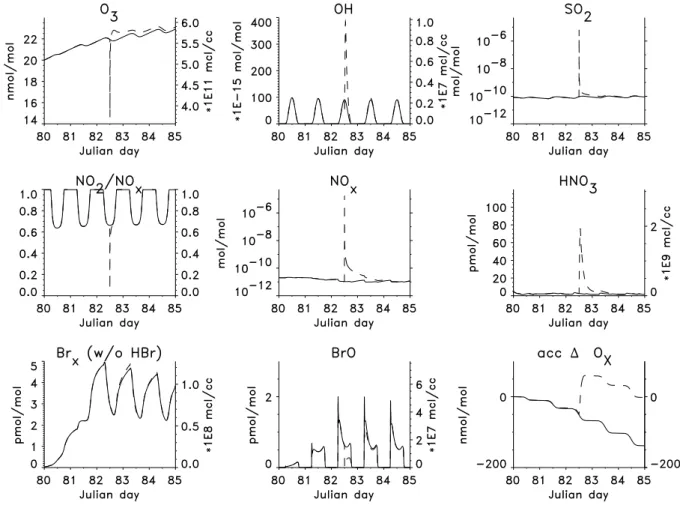
Fig. 2.Development with time of the major gas phase species and accumulated1Oxin undisturbed background air (solid line) and plume air (dashed line). Emission of the ship plume is at 12:00 on the third day (=Julian day 82). Note that immediately after plume release almost all O3is destroyed which is not shown on the figure due to an output timestep of 5 minutes.
The use of the values for effective uptake coefficients (γ) as accommodation coefficients (α) might lead to an underesti-mate of the overall loss rate. We tested this and found that the differences in loss rate coefficients were less than 1%.
Note that (Kirchner et al., 2000) found distinctly smaller uptake coefficients for NO2for various types of soot, but
es-pecially for diesel car soot which is thought to be most rep-resentative for ship emissions. Therefore the estimates that we used are clearly upper limits. According to Kamm et al. (1999) and Disselkamp et al. (2000) we do not assume het-erogeneous uptake of O3 on soot. The surface of soot and
therefore the uptake properties are subject to changes during the atmospheric lifetime of soot. Due to incomplete knowl-edge of this process we assumed no dependence with time of the uptake reactions.
We want to stress that still a lot of information on het-erogeneous reactions on carbonaceous/soot aerosol particles is uncertain or missing which makes an assessment of these processes difficult. Therefore we chose for most parameters (emission strength, plume dilution, time of plume release,α
etc.) the values in such a way that we get a best possible
estimate or, if the data were too uncertain, an upper limit.
3 Effects of emissions of a single ship
In this section we discuss in detail the chemical devlopment of the exhaust plume of a single ship. We investigated the ef-fects of different initial values of the background NOxand O3
concentrations (Sect. 3.2), of the local time of plume emis-sion (Sect. 3.3), of different plume expanemis-sion rates (different values forα, Sect. 3.4), of aerosol chemistry (Sect. 3.5), and of the emissions strength and NO:NO2ratio (Sect. 3.6). All
model runs were made for cloud-free conditions. To be able to concentrate on effects of changing individual parameters we chose to use the same meteorological conditions for all runs that we describe here. The temperature is 15◦C, the rel-ative humidity 81% and the depth of the marine boundary layer is 750 m. The photolysis rates are calculated for a ge-ographical latitude of 45◦ with an O3 column of 300 DU.
3.1 Base run
The base run includes background aerosol particles as well as emission of partly soluble particles (1.82×107cm−3one second after puff release) and soot particles (1. ×105cm−3 one second after puff release). The ship plume is emit-ted at 12:00 local time on the third model day to allow a model spin-up time of 2.5 days. The initial NOxmixing ratio
([NOx]0) is 20 pmol mol−1 and the initial O3mixing ratio
is 20 nmol mol−1. We included a constant O3source of 2.3
pmol mol−1day−1to yield approximately constant O3
con-centrations after the halogen chemistry has fully developed. Chemical reactions lead to a net chemical O3destruction as
explained below. All C2 and higher alkanes and alkenes are lumped with initial mixing ratios of 500 pmol mol−1 and 50 pmol mol−1, respectively.
Figure 2 shows a comparison of the evolution of the mix-ing ratios in background and plume air. In all of the studied cases the overall evolution of the plume air is similar: O3is
destroyed immediately after plume release by reaction with NO, minimal mixing ratios are close to zero in the first few seconds after plume emission. This is not visible in the plot as the output timestep is 5 min and by this time O3 has
al-ready been reformed and entrained. Later O3is produced by
NOxcatalyzed hydrocarbon oxidation reactions. The
maxi-mum increase in O3in the plume air compared to the
back-ground air is small, about 1 nmol mol−1 (i.e. 5%). Di-rectly after plume emission[OH]decreases due to the strong emissions of CO but then OH is reformed by the reactions HO2+NO and CH3OO+NO. The maximum value of OH
is 1.1×10⁷molec cm−3(i.e. 340% increase) on the first day immediately after plume emission. The maximum increase in HNO3is about 70 pmol mol−1. Maximum mixing ratios
are 18µmol mol−1for NO
x and 6.5µmol mol−1for SO2,
these are determined by the assumed exhaust mixing ratios. Immediately after release of the “puff” the NOxmixing ratios
are dramatically reduced, mainly by expansion of the plume. Chemical loss of NOxoccurs via the production of HNO3as
a product of the reaction OH+NO2. HNO3is then either
deposited on the sea surface or taken up by particles. To evaluate the production of ozone, the odd oxygen fam-ily Oxis defined based on Crutzen and Schmailzl (1983): Ox
= O3+ O + O(1D)+ NO2+ 2 NO3+ 3 N2O5+ HNO4+ ClO
+ 2 Cl2O2+ 2 OClO + BrO. The accumulated change in Ox
(shown as “acc1Ox” in the figures) accounts only for
chem-ical Oxdestruction and production. In the background air net
chemical Oxdestruction occurs due to the low NOxmixing
ratios. After plume release there is a large difference in net chemical Oxchange between the background and plume air,
with production in the plume. Most of this production oc-curs in the first few hours after plume release. For the base run the increase in Oxis about 3 nmol mol−1(note that the
accumulated Ox rates in the plots do not show the titration
of O3by NO in the early plume stage because the produced
NO2is part of the Oxfamily).
As a consequence of the uptake of HNO3by the sea salt
aerosol, acid displacement occurs and HCl degasses from the sea salt aerosol, increasing the HCl mixing ratio from about 10 pmol mol−1 to a maximum of 35 pmol mol−1 in the fresh plume. Through a series of reactions (see Sander and Crutzen, 1996; Vogt et al., 1996; Fickert et al., 1999) re-active bromine and chlorine species are released from sea salt aerosol, that might have an influence on the gas phase chem-istry. Also, the high NOx reactions initiate reaction cycles
involving halogenated nitrogen oxides (see Finlayson-Pitts and Hemminger, 2000, for an overview).
In the model an autocatalytic cycle takes place under clean conditions that leads to the release of bromine (Br2,BrCl)
from the sea salt aerosol. These species photolyze, produce the Br radical, which subsequently reacts with O3, forming
BrO. BrO reacts with HO2to HOBr which is taken up by the
aerosol thereby closing the reaction cycle. For more details see Sander and Crutzen (1996), Vogt et al. (1996), or von Glasow et al. (2002c). In the fresh plume, BrO mixing ratios decrease due to the high NO concentration in the reaction: NO+BrO−→NO2+Br.
This reaction reduces BrO strongly but it has no net effect on Oxbecause both BrO and NO2are members of the Ox
fam-ily. In the reaction of BrO with NO2, BrNO3is formed and
further reactions involving the aerosol phase (Sander et al., 1999) can lead to formation of HOBr and the liberation of Br2and BrCl from the particles and the subsequent loss of
Oxby halogen reactions.
This bromine activation cycle, however, cannot balance the decline in HOBr production by BrO+HO2, as both BrO
and HO2 are strongly reduced in the highly concentrated
plume. The production of HBr in the plume leads to a de-crease in Brx (which is the sum of all gas phase bromine
species except HBr) on the first day after plume emission. Only later when NO mixing ratios are already small due to dilution, an increase in Brx in the plume compared to the
background can be seen in all runs except for the one with slow plume evolution. This is caused by reactions involving BrNO3.
Through reactions on the sea salt surface and reactions in the gas phase, Cl2 is also formed in the plume air, where
mixing ratios are up to twice as high as in the background air. The concentration of Cl increases from 103atoms cm−3 to a maximum of to 3×10⁴atoms cm−3. This maximum is,
however, too short lifed to be of importance for the chemistry. Differences between background and plume concentra-tions of more than 10% are present for OH only on the first day and for SO2, NOx and HNO3 on the first and second
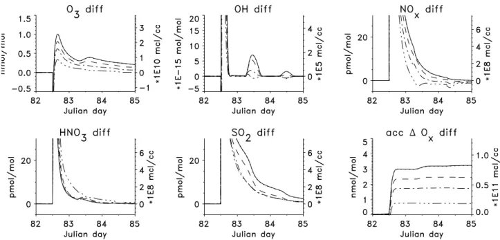
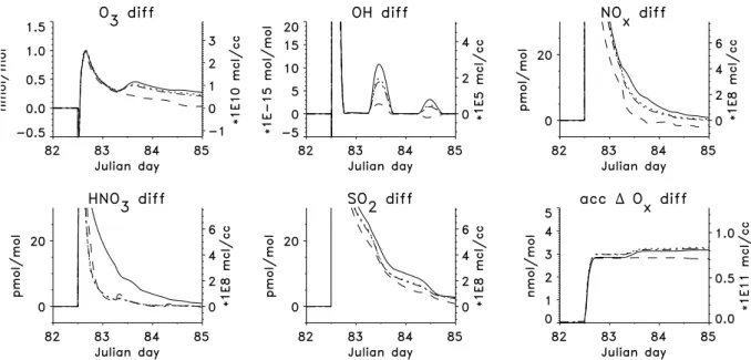
Fig. 3.Differences between plume and undisturbed background air in the evolution with time of the major gas phase species and accumulated Oxproduction rates for emission of a ship plume at 12:00 on the third day (=Julian day 82). The lines show runs with different background NOxmixing ratios: solid line: 5 pmol mol−1; dotted: 20 pmol mol−1; dashed: 100 pmol mol−1; dash-dotted: 200 pmol mol−1; dash-dot-dot: 500 pmol mol−1. The difference between the run with 5 and 20 pmol mol−1is barely visible. The initial background mixing ratio of O3is 20 nmol mol−1and that of SO2is 90 pmol mol−1.
2 days. Note that the mean lifetime of 7.3 h that was derived during the MAST campaign (Durkee et al., 2000a) is based on a different definition, namely on cloud albedo effects as measured from satellites. The most dramatic reductions in pollutant concentrations of course occur during the first hour after plume release. Our definition of chemical lifetime is meant to indicate when an airmass that was influenced by a ship can no longer be distinguished from one that was not perturbed. It has to be stressed that this result is strongly dependent on atmospheric mixing (see Sect. 3.4).
It is important to point to the differences in NOxlifetime
in the early plume stages. The instantaneous lifetime is re-duced from about 17.5 h in background air to 4.5 h in plume air directly after plume emission. See also Sect. 4.2 for fur-ther discussion of the NOxlifetime and comparison to the
lifetimes if the plume is treated as a continous source. The lifetime of SO2is influenced less because loss via
ox-idation by OH is only a minor factor. In background air its lifetime against oxidation by OH is of the order of 10 days and if oxidation in aerosol particles is included it is still about 7 days (all data from von Glasow et al., 2002b). In cloud free plume air the instantaneous lifetime of SO2against oxidation
by OH is reduced by only 50%. 3.2 Background NOxand O3
We varied the background NOx mixing ratios between 5
pmol mol−1 and 500 pmol mol−1. In the runs with high
initial background concentrations of NOxthese high values
were artificially sustained by corresponding NOxsources to
see the effect of ship emissions in high NOx regimes, e.g.
coastal regions. For runs with initial NOx mixing ratios
above 50 pmol mol−1, O3is produced in the background air,
in the runs with lower initial NOx, O3is destroyed.
In Fig. 3 the evolution with time of the major gas phase species for the runs with initial NOx mixing ratios of 5 to
500 pmol mol−1is depicted. Shown are the differences be-tween undisturbed background and plume air (e.g. O3diff).
Parts of the graphs are outside the plotting region, because the maxima are mainly determined by the in-plume values and for our discussion the plume development after the first few hours is most relevant and not the maximum differences. The maximum increase in [OH] is between 7.5 ×10⁶ molec cm−3for the run with[NOx]= 5 pmol mol−1and 2.8
×106molec cm−3for the run with[NOx]= 500 pmol mol−1 on the second day after plume release. The difference in NOx
between background and plume air is reduced quicker in the cases with high initial NOxconcentrations because more
HNO3is produced due to the higher OH concentrations. The
maximum increase in HNO3is about 70 pmol mol−1for the
run with [NOx]= 5 pmol mol−1 and 100 pmol mol−1 for
the run with[NOx]= 500 pmol mol−1. Note that in the runs
with higher initial NOx mixing ratios there is less NOx in
ship derived partly soluble sulfate particles and subsequent reactions among the different NOyspecies.
Naturally the change in the Ox budget due to the ship
emissions of about 0.8 to 3 nmol mol−1on the first day af-ter plume release is less important for the runs with already high Ox production. For the runs with net O3 destruction
in the background air (i.e. runs with initial NOx below 50
pmol mol−1) this is a major change in the chemistry because the system moved in the plume air from Oxdestruction to Ox
production. For the NOx= 5 pmol mol−1run the background
Oxdestruction is roughly 0.8 nmol mol−1day−1whereas for
the NOx= 500 pmol mol−1run the background Ox
produc-tion is about 5.6 nmol−1day−1. Note that not only the rela-tive but also the absolute changes in O3and other trace gases
are less pronounced in the runs with high initial NOx. This
is caused by the high background NOx concentrations that
already lead to significant Oxproduction and high O3levels
in the background. These need to be replenished by chemi-cal production and entrainment after the titration of O3in the
first minutes after plume release.
Effects on NOx lifetime reduction in the plume are a lot
less pronounced in the runs with high[NOx]0because of al-ready high OH concentrations in the background air. In the run with[NOx]0=500 pmol mol−1the OH concentration at
noon before plume emission is about 1×10⁷ molec cm−3 implying an instantaneous NOxlifetime of 3.6 h. The
rela-tive increase of [OH] is only 14% (compared to 330% in the base run) and the decrease of the NOxlifetime is only about
15%.
In summary, the impact and lifetime of ship emissions are largest for the run with the smallest NOxbackground mixing
ratios. The reason for this lies in the small OH concentrations for the runs with low NOx. As OH is the most important gas
phase sink for NOxand SO2, these low background
concen-trations of OH result in the largest differences between plume and background concentrations of NOxand SO2in the runs
with smallest initial NOxmixing ratios.
A similar result was found when the initial O3mixing ratio
was varied between 10 and 50 nmol mol−1(not shown). The effects of ship emissions are strongest and most persistent for low O3regimes.
3.3 Plume emission time
When ship emissions occur during night, NO3 and N2O5
(which is taken up by the particles) are formed and due to the lack of OH the transformation of NOx to HNO3 is
slowed down compared to cases with emissions during the day. We did runs with plume emission time at 6:00, 12:00 (base run), 18:00 and 24:00 local time. Overall the effects are more pronounced when emissions occur during day when the photochemistry is active. Accumulated Ox production
de-creased from about 3 nmol mol−1in the base case to roughly 0.5 nmol mol−1in the case with plume release at 18:00 lo-cal time. Peak mixing ratios of HNO3 decreased also
sig-nificantly to about 20 pmol mol−1if the emission occured
during night. The “slower” chemistry during night (due to the lack of photochemistry) increases the importance of en-trainment of background air. The decrease of NOxand SO2
is similar for all runs indicating that during the first day this is mainly determined by dilution of the plume.
When emissions occur during night, when the lifetime of most species is greater than during the day, reservoir species can be formed in the plume air. They have the potential to be transported to regions that have previously been unaffected by ship emissions. Reservoir species can also be formed in cold regions from species that are mainly destroyed by ther-molysis (similar to PAN). Therefore the longrange effect of ship emissions would be most pronounced in high latitude winters.
3.4 Influence of mixing
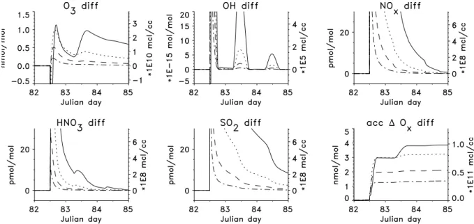
To study the influence of dilution on the evolution of the plume, different values for α, the horizontal plume expan-sion rate, were used. Values ofα = 0.62 (plume width af-ter 2.5 days = 20 km), α = 0.75 (100 km, “best guess”),
α=0.87 (438 km), andα=1.0 (2160 km) were used (see Fig. 4). All these runs were done with background mixing ratios of O3= 20 nmol mol−1and NOx= 20 pmol mol−1.
In the case of α = 1.0 mixing is very quick and 1 day after plume emission background and plume air cannot be distinguished anymore.
For α = 0.62 the opposite is the case, mixing is very slow and in most species differences between background and plume air are visible on the third day after plume release. The conversion of O3to NO2on the first day after plume
re-lease is very strong (note that[Ox]remains constant during
this conversion), and strong Ox production is still occuring
on the second day after plume release.
The maximum OH concentrations in the plume are 6×10⁶ molec cm−3 for the run withα = 0.62 and about 9×10⁶ molec cm−3 for the run withαvalues between 0.75 and 1. The maximum[HNO3]are 170 pmol mol−1for the run with
α = 0.62, 80 pmol mol−1for the run with α = 0.75, 25 pmol mol−1for the run withα= 0.87 and 15 pmol mol−1 for the run withα=1.
The results from the runs withα=0.62 are unrealistic be-cause such a strong and persistent separation between plume and background air is not expected to occur in the MBL. On the other hand, the very strong mixing in the runs with
α > 0.82 is not consistent with the observed persistence of ship tracks and probably only valid for extremely turbulent cases, so that our “best guess” of theαis likely appropriate.
Fig. 4.Same as Figure 3, but for runs with different plume expansion rates: solid line:α=0.62, dotted:α=0.75 (”best guess”), dashed:
α=0.87, dash-dotted:α=1. For these runs the initial O3mixing ratio is 20 nmol mol−1, that of SO2is 90 pmol mol−1and that of NOx is 20 pmol mol−1.
the order of 10−5, so then mixing is only relevant for species with very large gradients between plume and background air. A consequence of this is that processes that sustain high concentrations of the pollutants in the first hours of plume evolution lead to higher levels of pollutants in the plume later on. The height of the MBL defines the maximum height to which the pollutants can rise without extra buoyancy, be-cause the inversion at the top of the MBL provides a bar-rier for the vertical transport of pollutants. A shallow MBL means that the pollutants are confined to a smaller volume of air and therefore the concentrations are higher. As relative changes in concentrations due to entrainment of background air are strongest in the first hours after plume release, a shal-lower MBL has the same net effect as small values ofαfor the horizontal mixing although the magnitude of the changes due to different MBL heights is smaller (not shown).
Diurnal variations in the height of the MBL might lead to the export of pollution into the free troposphere, where the potential for long-range transport of reservoir species exists. This process might also lead to faster loss of NOxfrom the
MBL. This would need to be to be addressed with a highly resolved 3D model (LES model).
3.5 Effects of aerosol chemistry
To study the effects of aerosol chemistry on the evolution of the ship plume we did runs with background aerosol only; with the additional emission of partly soluble particles (the soluble part is assumed to be H2SO4); with the additional
emission of both partly soluble particles and insoluble soot
Table 3.Description of the different runs including aerosols
case partly soluble particles soot particles
run 2 1.82×107cm−3 none run 3 1.82×108cm−3 none
run 4 1.82×107cm−3 1.×105cm−3 run 5 1.82×107cm−3 1.×107cm−3 run 6 1.82×108cm−3 1.×107cm−3
particles from the ship (= base run); and without inclusion of aerosols.
The runs were made for an initial O3mixing ratio of 20
nmol mol−1and initial NOxmixing ratio of 20 pmol mol−1.
Run 0 is with gas phase chemistry only and run 1 with background aerosols only. The total surface areas for the background sulfate and sea salt particles are 1.75 ×10⁻⁵ m2m−3and 3.38×10⁻⁵m2m−3, respectively. We compare these runs and runs with the concentrations of ship-derived particles one second after plume release as listed in Table 3.
The initial surface areas of partly soluble ship particles are 0.568 m2 m−3 and 5.68 m2 m−3 for the low and high
es-timates, respectively, whereas they are 2.6×10⁻³m2m−3
Fig. 5.Same as Fig. 3, but for runs including aerosol chemistry: solid line: no aerosol chemistry (run 0); dotted: background aerosol only (run 1); dashed: additionally partly soluble ship particles, concentration 1 second after plume release: 1.82×108cm−3(run 3); dash-dotted: additionally partly soluble ship particles (1.82×107 cm−3) and soot particles (run 4 = base run). For all runs the initial NOxwas 20 pmol mol−1and O3= 20 nmol mol−1.
of ship derived particles comparable to the number of back-ground particles for a time span that is long enough to ensure that heterogeneous reactions can show an effect. For run 2 the number of ship derived particles equals the number of background particles after about 4.4 h. For run 3 this is the case after 2.37 days.
The overall qualitative evolution of the gas phase species in the plume air in runs 1 to 6 is similar to the base run that has been discussed previously. The differences between runs 2, 4, and 5 are negligible as are the differences between runs 3 and 6. This means that the effect of soot aerosol on the evolution of the gas phase chemistry is negligible. Even the very high soot concentrations in runs 5 and 6 did not show any importance of the soot aerosol. This can be un-derstood by looking at the rate coefficients and associated lifetimes. The highest accommodation coefficient was as-sumed for HO2, withαHO2 =10
−2. In the first second after
plume emission the lifetime of HO2 against uptake on soot
isτsoot = 357 s for a soot concentration of 1 ×105 cm−3
after 1 second. Two minutes after plume release the life-time increased toτsoot=0.86 days already. The lifetime of
HO2 against reaction with NO at an NO mixing ratio of 1
nmol mol−1is aboutτNO2 =4.8 s (at 290 K, DeMore et al., 1997). In the early plume stages the NO concentration is a lot higher than this value. This indicates that even with our up-per limit estimates of reaction rates, soot aerosol in the ship plume has no effect on gas phase chemistry.
In Fig. 5 we compare runs 0, 1, 3, and 4. The overall ef-fects of aerosol particles on the chemistry in a ship plume in the cloud-free MBL are important for some species
accord-ing to the model. In run 3 the chemical lifetime of the ship plume is reduced substantially, which can easily be seen, e.g. in the small OH and NOx differences between plume and
background air. As in the runs with high initial NOxmixing
ratios loss of NOyon ship derived sulfate particles leads to
smaller NOxmixing ratios in run 3 than in the background.
The decline in HNO3is similar for all runs with aerosols
be-cause it is mainly taken up by sea salt aerosol.
SO2evolves similarly in all runs including the gas phase
only run. This indicates that its main sink in the plume is dilution and not uptake on the particles, which is con-firmed by a lifetime of the order of 30 h, at [OH] = 1
×107molec cm−3, (DeMore et al., 1997). Its oxidation prod-uct H2SO4is taken up by the particles, increasing the S(VI)
content of the aerosols by a few pmol mol−1(3 to 10% for the background aerosols).
In the runs with the emission of very high numbers of ship derived particles (runs 3 and 6), there is enough surface avail-able to convert BrNO3 and HBr to more reactive bromine
species. Therefore in these runs no drop in Brxoccurs after
plume release (not shown).
In summary, the emission of soot particles from ships with the characteristica that we assumed is unimportant for the chemistry of the cloud-free MBL and only very high particle emission rates of partly soluble particles as in run 3 lead to disturbances of the chemistry that are distinguishable from the effect of background aerosol particles.
similar plume expansion approach as described here. The re-sults show a strong influence of the state of coupling between cloud and sub-cloud layers. If these layers are coupled, the soluble gases that are emitted are rapidly scavenged. If cloud and sub-cloud layers are decoupled then the emissions are confined to a rather small region leading to higher mixing ratios of pollutants (and Cl2 and HCl) than in a cloud-free
case. Upon coupling of the cloud and sub-cloud layers these differences disppeared quickly. An obvious conclusion from this study was that the lifetimes of soluble pollutants (e.g. SO2) are reduced in a cloudy MBL, whereas those of
insol-uble pollutants are roughly the same as in cloud-free cases. Furthermore differences in aqueous phase chemistry due to the emission of soluble particles and sulfur compounds can be expected. Based on these results, our box model calcula-tions that were performed for the cloud-free MBL provide an upper limit of the effects in the atmosphere.
3.6 Emission strength and NOxpartitioning
We did further sensitivity studies where we varied the ship emissions by a factor of 0.1 and 10, respectively. In the case of a reduced emission strength, the chemical plume lifetime was reduced to about 12 h, whereas it was longer than 3 days if the emission strength was increased.
EPA (2000) gave a NO:NO2 ratio for the exhaust air of
96:4. We tested the implications of a higher fraction of NO2
in the plume air. As expected, a higher NO2fraction leads to
O3formation by photolysis of NO2. This effect is, however,
important only in the first 100 s after plume release and of no importance for the later evolution of plume air. After this time the O3that was derived from NO2photolysis is diluted
by entrainment of background air and the NO:NO2 ratio is
about 0.8 for our base case as well as for NO:NO2emission
ratios of 20:80, 50:50 and 80:20. If the emission occurs dur-ing night, the NO:NO2emission ratio is of no importance, as
all NO reacts very quickly to NO2.
4 Effects of emissions of several ships and of plume overlap
So far the emissions of only one ship have been considered. To be able to extrapolate these results to a more global pic-ture, the effects of the emissions of several ships have to be discussed. In Sect. 4.1 we explore the plume overlap in the framework of our model and compare our results in Sect. 4.2 with the approach used in global models. It has to be em-phasized that our extrapolation method is only one of several possibilities.
4.1 Upscaling approach
From the emissions inventory of Corbett et al. (1999) annual mean emission fluxes (mass nitrogen, sulfur) per area and time can be extracted. If the emissions rate of one ship is
known, the number of ships per area that are needed to pro-duce the emissions as they are listed in the inventory, can be calculated. For the most frequently crossed ocean re-gions (North Atlantic and North Pacific) values from Corbett et al. (1999) are about 10−9 g(N) m−2 s−1 for a fleet that emits on average 22.7 g(N) kg−fuel1. Hobbs et al. (2000) give a mean fuel consumption of 0.84 kgfuel s−1 (median = 0.69
kgfuel s−1) for ships studied during the MAST campaign.
They estimated the fuel consumption from the nominal en-gine power as listed in ship registries and the observed ship speed. Fuel consumption rates can also be estimated from EPA (2000), that give an average fuel consumption of 223 gfuelkWh−1. Assuming an engine power of 16 MW, which
is the average of the engine power during MAST (median = 13.4 MW), this would result in a fuel consumption of 0.993 kgfuels−1, similar to the estimate from Hobbs et al. (2000).
For the further discussion we make use of emissions by an “average ship” based on previously listed mean values which are higher than the medians. According to Corbett et al. (1999) 42% of the ships cause 70% of the total annual nitrogen emissions. Clearly, the global fleet of ships consists of small and large ships with different emissions characteris-tics. It would be best to take this into account which, how-ever, cannot be done in the type of study that we did.
Based on these data an “average ship” emits 19.1 g(N) s−1. This leads to 5.24×10⁻¹¹ships m−2that have to be present all year round in the more frequently crossed regions to pro-duce the emissions that were estimated by Corbett et al. (1999). Taking the uncertainty of this estimate into ac-count, sensitivity studies are made using values from 1 to 10×10−11ships m−2.
To estimate the impact of several ships in an area of a cer-tain size the following assumptions are made: i) All ships are homogeneously distributed over this area because the ocean regions considered are quite large and different destinations lead to different ship routes. ii) As most traffic in the more frequently traveled oceans crosses these regions from Asia to North America and from North America to Europe (or in the opposite direction) all routes are parallel.
For convenience the following calculations are based on the emissions of ships in a certain area. The size of this “cell” is determined by the distance that a ship travels during the chemical lifetime of its plume. During these 2 days a ship that has a speed of 10 m s−1travels 1730 km. We use this
as length of a cell which, for convenience, we chose to be quadratic. In the chosen cell area of 1730 km by 1730 km between about 30 to 300 ships are cruising at any point in time based on the “ship density” given above. Two days after plume emission the plume width iswpl =85 km usingα= 0.75 (see Eq. 1). Therefore the area that is influenced by one ship in 2 days is about 7.4×10¹⁰ m2(approximately 0.5×
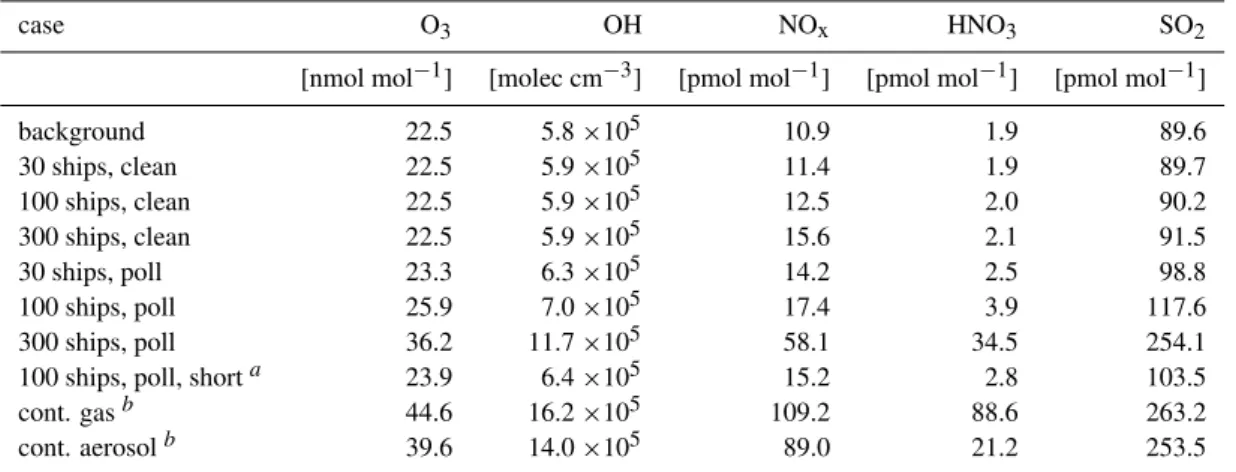
Table 4.Extrapolation of different scenarios.
case O3 OH NOx HNO3 SO2
[nmol mol−1] [molec cm−3] [pmol mol−1] [pmol mol−1] [pmol mol−1]
background 22.5 5.8×10⁵ 10.9 1.9 89.6
30 ships, clean 22.5 5.9×10⁵ 11.4 1.9 89.7
100 ships, clean 22.5 5.9×10⁵ 12.5 2.0 90.2
300 ships, clean 22.5 5.9×10⁵ 15.6 2.1 91.5
30 ships, poll 23.3 6.3×10⁵ 14.2 2.5 98.8
100 ships, poll 25.9 7.0×10⁵ 17.4 3.9 117.6
300 ships, poll 36.2 11.7×10⁵ 58.1 34.5 254.1
100 ships, poll, shorta 23.9 6.4×10⁵ 15.2 2.8 103.5
cont. gasb 44.6 16.2×10⁵ 109.2 88.6 263.2
cont. aerosolb 39.6 14.0×10⁵ 89.0 21.2 253.5
Mean mixing ratios in a cell of 1730 km by 1730 km. 30 ships in this area correspond to an emission of 2.7×10⁻¹⁰g(N) m−2s−1, 100 ships correspond to 1×10⁻⁹g(N) m−2s−1and 300 ships to 2.7×10⁻⁹g(N) m−2s−1, respectively. In the “clean” cases background air is mixed into the plume, whereas in the “poll” cases air that has been influenced by a previous ship is mixed into the plume. For a description of the “poll” cases see text. In the “background” case no ship emissions are considered. Plume lifetime for these runs was 2 days.
aRun with a chemical plume lifetime of 1 day (α=0.87,β=0.65). The area of the cell used for averaging was adjusted.
bSteady state values from the runs discussed in Sect. 4.2. Using a similar scaling approach as for the data in Table 2 emissions for CO were
estimated to be 4×10⁸molec cm−2s−1and 2×10⁷molec cm−2s−1for HCHO.
polluted by previous ships.
Based on these estimates, we discuss seven mixing scenar-ios: low, best guess and high emission rates (i.e. 30, 100 and 300 ships per cell of 1730 km by 1730 km), each case with plume emission in background air and air that had been in-fluenced by previous ships, and one with 100 ships, emission in prepolluted air, but with a reduced plume lifetime.
For the runs in pre-polluted air we assume that after emis-sion of a first plume no background air but only air that had been influenced by a previous plume is entrained. The time lag between plume emissions is calculated based on the num-ber of ship plumes that overlap in the different cases. In the best guess (“100 poll”) scenario 2.5 plumes overlap, there-fore the time lag, based on a chemical lifetime of the plume of 2 days is about 19 h. This results in increasing pollu-tion levels in both the “plume” and “background” air masses that we consider in our box model (see Sect. 2) and after a few days steady state mixing ratios are established. Note that this approach differs from the one used in von Glasow et al. (2002a). We have to stress that these results are based on assumptions that involve substantial uncertainties, espe-cially the plume dispersion will be different in specific ship plumes. Our upscaling results are not supposed to give final answers, they are more pointing to research needs and to give an idea of effects on a global scale. The use of box models for upscaling can only give first ideas, it cannot replace further studies with high-resultion 3D models (i.e. LES models).
Table 4 shows the resulting mean mixing ratios for runs with (“poll”) and without (“clean”) overlap of ship plumes. The “30 ships, clean” case which corresponds to an
emis-sion flux of 1.9 ×10⁻¹⁰ g(N) m−2 s−1 can be seen as
most relevant for less heavily traveled regions and the “100 ships, poll” case which corresponds to an emission flux of 6.4 ×10⁻¹⁰ g(N) m−2 s−1 as most relevant for the North Atlantic and North Pacific. For coastal regions the “300 ships, poll” case might apply (emission flux of 1.9×10⁻⁹ g(N) m−2 s−1). According to these results the lower limit scenario with emissions into background air (“30 ships, clean”) would be nearly indistinguishable from the back-ground air. The high emission scenario with entrainment of clean background air (“300 ships, clean”) would increase OH by 2%, NOx by 43% and SO2 by 2% compared to a case
without ship emissions.
The effects of emission into prepolluted air are more ap-parent, especially for the upper limit scenario (“300 ships, poll”). Here O3is predicted to increase by 60% compared to
background air, OH would increase by 100%. NOxwould
in-crease by a factor of 5.3 and SO2by 187%. In the best guess
scenario (“100 ships, poll”), O3would increase by 15%, OH
by 21%, NOxby 60% and SO2by 31%.
The run with enhanced entrainment of air into the plume (“100 ships, poll, short”, for conditions in the North Atlantic and North Pacific) shows a decrease of the effect of ship emissions with the overall effects being close to the lower limit scenario (“30 ships, poll”).
MBL might by overestimated by global models compared to measurements. To check this we performed additional runs (with and without aerosol chemistry) with our box model. These runs include the chemistry that we described earlier but no plume expansion is considered. Instead ship emis-sions are treated as in a global chemistry transport model by assuming a continuous source of the ship pollutants. The emission fluxes are the same as in the best guess scencario (“100 ships” case).
These runs show significant production of Ox. The steady
state mixing ratios for O3are about 40 and 45 nmol mol−1
(including a continuous source as in the other runs) for the runs with and without background aerosol chemistry, respec-tively, compared to 25 and 29 nmol mol−1for the same runs without ship emissions. The mixing ratios of OH are more than doubled.
NOxlevels increased to 110 pmol mol−1in the run without
aerosol chemistry and to 90 pmol mol−1in the run including aerosol chemistry compared to 10 pmol mol−1in the back-ground and 46 pmol mol−1 in the best guess scenario with plume overlap (“100 ships, poll”). The difference in steady state between these 2 runs of about 20 pmol mol−1implies an additional sink of roughly 20 pmol mol−1day−1in the run including aerosol chemistry. The heterogeneous reactions re-sponsible for this difference are uptake of NO3, N2O5, and
XNO3 (X = Cl, Br) on the aerosol. In the model the most
important path is uptake of BrNO3on the sulfate aerosol
ac-counting for roughly two-thirds of the total loss of NOx.
The results for NOx, OH and O3from these runs (see
Ta-ble 4) are similar to but somewhat smaller than the numbers from global models (Lawrence and Crutzen, 1999; Kasib-hatla et al., 2000). Chemistry on aerosol particles appears to explain only part of the great differences between measure-ments of NOxin the MBL and global model results.
Comparing the results with constant emissions with the steady state concentrations as discussed in the previous sec-tion (“cont, aerosol” vs. “100 ships, poll”), differences of about a factor of 5 in HNO3and NOxand a factor of 2 in OH
and SO2 are apparent. As already mentioned at the end of
Sect. 2.1, the dilution of plume air does not affect the mass balance of the emitted species because dilution in the model is only by entrainment of background air and not by detrain-ment of plume air.
As suggested by Dentener (2002) we made a consistency check of our extrapolations by decreasing the emissions per ship and increasing at the same time the number of ships thereby approaching the “constant emissions” approach of global models. In our upscaling runs it is implicitly assumed that for plume dilution only the last preceding plume is of importance and that for that plume dilution and/or entrain-ment is not important at all. If ship emissions are assumed to occur very frequently (i.e. order of an hour or less apart) this assumption is not correct any more. As stated in Sect. 3.4 the “rapid mixing time” ends after about 6 h and if emissions are reduced such that ship frequency is still more than 6 h, the
proposed consistency test (distribution of the emissions to 3 times more ships) shows a convergence of the “100 ships, poll” run towards “cont, aerosol”. It fails, however, for an increase of the number of ships by a factor of 10 or 30, be-cause then the time between plume emissions is on the order of or shorter than 1 hour and the implicit-dilution assump-tion is not valid anymore. Furthermore, a reducassump-tion in plume emission strength also leads to a reduction of plume lifetime. This has to be accounted for in the calculation of time lag between ships which on the other hand implies that it would not be as strict of a consistency test as could be hoped.
As suggested by Davis et al. (2001) for differences be-tween measurements and global model results, the differ-ences between our upscaling approach and our runs with con-stant emissions are related to the extremely high NOxmixing
ratios and very rapid dilution in plume air compared to con-stantly high NOxvalues in the air affected by a continuous
source. The differences are a result of different lifetimes of NOxin air with high NOxand OH concentrations (plume air)
and in air with moderate increases in these 2 species (contin-uous emissions).
The lifetime of NOx in the early stages of the plume is
strongly reduced compared to background situations. Peak concentrations of OH in the plume are about OH=1.1×10⁷ molec cm−3. Using a rate coefficient of k = 9.1 ×
10−12cm3molec−1s−1(Sander et al. (2000) atp=1013.25 hPa,T =298 K), the NOxe-folding lifetime due to the
re-action NO2+OH−→HNO3would be about 2.76 h
com-pared to 14.7 h in the background air (based on an OH con-centration of about 2×10⁶ molec cm−3). As the
concen-trations of OH and all other species decrease rapidly in the first hours after plume emission, we calculated the following mean e-folding lifetimes (“mean lifetime”) for our base run with plume dilution. The mean lifetime of NOxin the first
6 h after emission of a plume at 12:00 is about 7.5 h in plume air compared to 26.9 h in undisturbed air, i.e. NOxis lost 3.6
times as fast as in the background air.
The mean lifetime of NOx in the runs with continuous
emissions between 12:00 and 18:00 (i.e. the same time span as given above) is 12.7 h, i.e. 1.7 times longer than in the run with description of plume chemistry. During the time of highest OH concentrations (5×10⁶molec cm−3) the e-folding lifetime of NOx is about 6.1 h, i.e. it is more than
2 times faster in the plume case. As NOx loss is strongest
in the first hours after plume emission, the large differences in NOx lifetime during this period are the main reason for
the differences between the two discussed emission scenar-ios (plume vs. continuous emissions). From these estimates it is obvious that the incorporation of the plume evolution is critical in assessing the effects of ship emissions.
Our results provide a first quantification of the conclusion of Davis et al. (2001) that reduced NOxlifetime in the ship
Song et al. (2002) uses a Gaussian plume dilution approach and finds similar effects on NOxlifetime as we do.
We want to add, that in the interpretation of field NOxdata
care has to be taken. From our studies it appears likely that only fresh plumes have NOxlevels that are significantly
ele-vated above background values, before it is converted to e.g. HNO3 and/or deposited. If these “NOx-spikes” are filtered
during processing of the data, important information is lost. This it is important to look for the variability of NOx, and
also of HNO3, in the data, similar to the use of medians in
Kasibhatla et al. (2000) and Davis et al. (2001), to get infor-mation about the impact of ship emissions on the chemistry of the MBL.
Therefore there is clearly a need for more data on global ship emissions, for measurements over the more heavily tra-versed ocean regions and for more information on additional chemical reactions that might occur in plume air.
In coastal regions or, e.g. in the oceans off Asia, where ship emissions are estimated to have grown by 5.9% per year between 1988 and 1995 (Streets et al., 2000) ship emissions definitely play a role for air quality, now and in the future.
5 Uncertainties
In the previous sections we already discussed the uncertain-ties of our model and upscaling approach. Another major uncertainty in this study is the estimate of the ship emis-sions. We mainly used the numbers from Corbett et al. (1999) that were already used in previously published stud-ies (Lawrence and Crutzen, 1999; Kasibhatla et al., 2000; Davis et al., 2001), so intercomparison between our and these studies is facilitated. Some of the data are confirmed by the compilation of EPA (2000). Also, Streets et al. (2000) show that their estimates for SO2emissions in Asian waters and
the respective data from Corbett et al. (1999) disagree only by 13%, which might be due to the fact, that Streets et al. (2000) did not consider fishing and military ships. Neverthe-less, it is important to consider the uncertainties which may be present in the data of Corbett et al. (1999).
For this purpose we estimated the average deployment time (time spent at sea) of a ship based on data given by Corbett et al. (1999).
The total annual world marine fuel usage from Table 2 in Corbett et al. (1999) is approximately 1.5×10¹¹kg. Accord-ing to Corbett et al. (1999) 42% of the ships cause 70% of the total annual nitrogen emissions. Based on this we assume that 42% of the ships also cause 70% of the total annual fuel consumption which leads to an average fuel usage for these ships of 2.5×10⁶kg ship−1a−1. With a fuel consumption of roughly 1 kg(fuel) s−1(EPA, 2000, see Sect. 4.1) this would mean that each ship would be operating 2.5×10⁶s or 29 days per year (or 17 days per year if all ships are consid-ered). This number is by far too small. According to Corbett et al. (1999) the deployment time of commercial ships is
con-siderably larger than their estimate of 50% deployment rate of military ships.
A similar estimate can be obtained by starting from our estimate (see Sect. 4.1) of the NOx emission per ship and
time of 19.1 g(N) ship−1 s−1 which results in 6 × 10⁸
g(N) ship−1 a−1 if it were continuously operating.
Con-sidering that 42% of the ships cause 70% of the total an-nual nitrogen emissions of 3×10¹²g(N) a−1(Corbett et al., 1999), these numbers combined would give a deployment time of approximately 30 days per year (or 18 days per year if all ships are considered), very similar to the estimate above (note that these estimates are only partially independent since the the total annual nitrogen emissions of 3×10¹²g(N) a−1 in Corbett et al. (1999) start from the total fuel usage of 1.5×10¹¹kg a−1).
The values of the nitrogen emission per ship and time calculated from measurements during the MAST campaign (Hobbs et al., 2000) are lower than the estimates from Cor-bett et al. (1999). They found values between 8.4 and 14 g(N) kg(fuel)−1(note that the range of this value is given incorrectly in the abstract and the text of their paper, while their Table 3 (NOxin mole(N) kg−1) gives the correct
num-bers (T. Garret, pers. comm. 2001, erratum accepted by J. Atmos. Sci.). The reason why these numbers are smaller than the other values from the literature (Corbett et al., 1999; EPA, 2000) is not yet resolved. Using them for the estimate of ship deployment rates would lead to deployment times of 41 to 68 days per year, which is still far too small. The data from EPA (2000), on the other hand, give an emissions rate of 22 g(N) s−1 (for a ship’s engine with 16 MW cruising at 80% load), which is similar to the number we calculated from Corbett et al. (1999).
Taking the above listed arguments together one could con-clude that either the emissions and fuel usage per ship or the number of active ships that were used in all cited studies (in-cuding this one) are too high. If the total number of registered ships and the other parameters are correct, this would imply that a much smaller fraction than 42% of these is actually active.
There is certainly still a great need for more data on the emissions of ships.
6 Summary and outlook
We studied the chemical evolution of the exhaust of ships in the MBL with a box model. Based on a simple dilution ap-proach for the plume we found the chemical lifetime (defined as time when differences between plume and background air are reduced to 5% or less) of the ship plumes to be about 2 days. Dilution has the strongest effects during roughly the first 6 h after plume release. For long lived species the dif-ferences that are present after this “rapid mixing period” are conserved. Given the predicted importance of entrainment of background air, our approach should be tested in the future against more detailed models of plume dilution (e.g. large eddy simulation models) and field data. Most field measure-ments did not follow a ship plume over its complete lifetime, which would be important to validate model results. This was done during the ITCT 2K2 campaign off California in 2002 and first results indicate very rapid dropoff in NOxand
NOyafter plume release which is unlikely to be explained by
OH-chemistry alone (Corbett et al., 2002).
The strongest effects of ship emissions and longest plume lifetimes were found when the emissions were into the clean-est background air. The lifetime of many species in the plume air is reduced due to high OH concentrations which are a consequence of the elevated NOx mixing ratios. This
fur-thers the conclusion of Davis et al. (2001) by quantifying the effect, and in particular by showing that it is sensitive to the background conditions, being strongest for remote back-ground regions.
We found the influence of background aerosol particles (sulfate and sea salt) to be important for the evolution of gas phase chemistry in the ship plume, whereas inclusion of solu-ble ship-produced aerosols was of little importance. We also used upper limits for reactions on soot aerosols and found re-actions on these particles to be unimportant for ship plumes. Chlorine is released significantly from sea salt aerosol in plume air. In our runs only minor additional (compared to the background) bromine release could occur because most bromine was already partitioned to the gas phase. In the early plume stages BrO reacts rapidly with NO thereby strongly reducing BrO mixing ratios but without a net effect on the Ox family as NO2 is produced in this reaction. Later on,
bromine is redistributed mainly towards BrNO3in plume air.
In more frequently crossed ocean regions like the North Atlantic or North Pacific and especially in coastal regions, the plumes of several ships overlap, so we considered the overlap of ship plumes in a simplified way. We found that the reduction of NOxlifetime in the ship plume can explain part
of the observed difference between open ocean NOx
mea-surements and predictions by global models, which treat ship emissions as a constant source. According to our extrapola-tion (best guess scenario – “100 ships, poll”), changes in O3
and OH (compared to background air) would be about 15 and 21%, respectively. The mixing ratios of NOx, HNO3
and SO2, however, would increase by 60%, 105%, and 31%,
respectively. These estimates are based on background mix-ing ratios of 20 pmol mol−1NOx and 20 nmol mol−1O3.
For cleaner regions, the effects of ships would be more pro-nounced. From our box model runs it is not possible to get a global perspective, so parameterizations for the plume dilu-tion should be developed and used in global models.
It should be noted that the limitations of global models to treat point sources correctly not only apply to ship emissions but to all types of point sources, e.g. land based power plant emissions.
We have also found some inconsistencies in current fuel usage and NOx ship emissions inventories, which have to
be clarified. Measurements of the chemistry and emissions directly in fresh plume air are highly encouraged to get reli-able data of ship emissions and of the chemical processes at different temporal distances from the emission. This should be done at the stack and from a second platform following at variable distance downwind from the studied ship. This could be a second ship, plane or especially an airship, which is slower than a plane, highly manoeuvrable and could also make vertical profiles in the plume as was done by Frick and Hoppel (2000) to study microphysical parameters of the ship track.
Apart from uncertainties in model assumptions or emis-sion inventories, other physical or chemical processes that were not included in our model might certainly be of impor-tance for plume development or differences between mea-surements and model results.
Ship emissions are a major source of anthropogenic pol-lution and the input of sulfur and nitrogen to the coupled ocean-atmosphere system is a major perturbation in these ar-eas which are usually affected only by advection of pollu-tants. Emissions from ships are potentially important (also for the cycle of sulfur which has not been the focus of this work) on large areas of our oceans, but especially in coastal regions. This study, among previous studies, indicates that much is left to be done. It is very important to gather more data on the emissions of ships and the chemical processes in ship plumes. In addition appropriate parametrizations for global models should be developed and further detailed stud-ies with process models of ship plumes should be made. Acknowledgements. We would like to thank Frank Dentener and Ulrich P¨oschl for helpful comments on this paper.
References
Ackerman, A. S., Toon, O. B., and Hobbs, P. V.: Numerical mod-eling of ship tracks produced by injections of cloud condensa-tion nuclei into marine stratiform clouds, J. Geophys. Res., 100, 7121–7133, 1995.