Optimization of reinforced concrete polygonal sections under biaxial
bending with axial force
Abstract
Concrete is the world’s most utilized material for production of the structural elements employed in civil construction. Due to its low tensile strength and brittle nature it is reinforced with steel bars forming the reinforced concrete (RC structure). Linear elements of reinforced concrete are commonly employed in multi-story buildings, bridges, industrial sheds, among others. In this study an optimization algorithm is presented to define the amount of steel and its loca-tion within a concrete polygonal secloca-tion subjected to biaxial bending with axial force, so that the amount of steel would be the minimum needed to resist the soliciting forces. Therefore, the project variables are: location, diameter and number of steel bars to be distributed within the concrete polygonal section. The sequential linear programming method is used to determine the optimized section. In this method, the non-linear problem of determining the resistance forces of the section in relation to the project variables is approximated by a se-quence of linear problems, which would have its optimal point defined for each step using the Simplex method. Formulation validation is done through results of examples found in literature, and also by means of analytical solutions of simple problems, such as rectangular sections under axial force and moment in only one axis of symmetry. The results show the efficiency of the algorithm implemented in the optimized determination of the quantity and position of the bars of a given diameter in the polygonal section of reinforced concrete under biaxial bending with axial force.
Keywords
optimization; RC polygonal section; biaxial bending; sequential linear progra-mming method.
1 INTRODUCTION
With increasing competition, there is an ever growing need to offer good quality products at a reduced cost. A use-ful tool to attend these needs is the optimization, or in other words, to define the maximum possibilities of a product or service. According to Maia (2009), the great advantage for optimizing projects is the abandonment of parameters based on the intuition or experience of engineers, emphasizing the searches for a solution by using an objective function to optimize the project, generally related with the execution and production cost of the project.
In our study, an optimization algorithm was implemented to define the amount of steel and its position within con-crete polygonal section subjected to biaxial bending with axial force, so that the amount of steel would be the minimum necessary to resist the soliciting forces, in addition to meeting the standard requirements referring to the reinforced con-crete member design according to ultimate limit states of bending with axial force (Eurocode 2, 2004, ABNT NBR 6118, 2014). That is, the main objective is given a polygonal section any and the soliciting forces define optimally the quantity, position and diameter of the steel bars. This optimization process utilizes a sequential linear programming method, where the non-linear problem to determine the resistance forces of the section in relation to the project variables is approximat-ed by a sequence of linear problem that has it optimal point definapproximat-ed for each step using the Simplex method.
To formulate this algorithm, a routine is used that is capable of supplying the resistance forces in the RC polygonal section. The routine has as input parameters: the shape of the RC cross-section, the positions and diameters of steel bars, the stress–strain diagrams for concrete and steel material, as well as the parameters of the cross-section deformation given by the plane equation, since being considered is the hypothesis for the maintenance of the plane section according to bending beam theory. This routine was developed by Sousa and Caldas (2005) and is being successfully utilized in the development of other studies (Sousa and Silva, 2007, Silva and Sousa, 2009, Sousa et. al., 2010, Sousa and Silva, 2010). In it an integration analytical method of applied to polygonal sections is used, alternative to the fiber method used in
Amilton R. Silvaa* Flávia C. Fariab
a Departamento de Engenharia Civil, Escola de
Minas, Universidade Federal de Ouro Preto - UFOP, Campus Universitário, Morro do Cruzeiro, Ouro Preto, MG, Brasil. E-mail:
bPrograma de Pós Graduação em Engenharia Civil,
Universidade Federal de Ouro Preto - UFOP, Ouro Preto, MG, Brasil. E-mail:
[email protected] *Corresponding author
http://dx.doi.org/10.1590/1679-78254252
several works (Hsu, 1985, Munoz and Hsu, 1997, El-Tawil and Deierlein, 2001). Sfakianakis (2002) developed an alter-native fiber model for the calculation of area integrals over RC section as well as composite steel–concrete sections. In this direction, several studies have been proposed for the analysis of resistance forces of arbitrary shape section under biaxial bending with axial force (Yau et. al., 1993, De Vivo and Rosati, 1998, Rodriguez and Aristizabal-Ochoa, 1999).
This subject is of great interest for civil construction and it is difficult to evaluate by simplified methods, which has motivated researchers to produce analysis tools for this type of problem (Rath et. al., 1999, Bastos, 2004, Junior, 2006, Bonet et. al., 2006). Guerra and Kiousis (2006) implemented a non-linear optimization algorithm that provides a solution for the minimum cost that satisfies the ACI 2005 code requirements for the designing of RC linear elements submitted to bending and axial loads. The authors used MatLab software to develop this tool. Similarly, other researchers have suc-cessfully used MatLab to solve optimization problems involving the analysis of RC elements undergoing combined ac-tion of bending moment e axial force (Ramos, 2011, Sias and Alves, 2014).
Just as herein, Silva et al. (2010, 2011) performed optimization of concrete-steel beams that were discretized in bar finite elements, using the sequential linear programming method associated with the Simplex method. Other authors have used the Simplex method with success for the optimization of a great number of engineering problems (Bona et. al, 2000, Anaut et. al, 2006). Other techniques for optimization of nonlinear problems of RC elements have been used in the literature, such as nonlinear programming (Balling and Yao, 1997, Camp et. al., 2003) and genetic algorithms (Mohar-rami and Grierson, 1993, Lee and Ahn, 2003). The contributions of this work are in the clear form as the analyzed prob-lem is modeled, in the detailing of the algorithm used, and also in the verification of the potentiality of a simple method (linear sequential programming) in the solution of constrained nonlinear optimization problem. This potentiality is veri-fied through the results obtained in the analysis of different cases.
2 FORMULATION OF THE PROBLEM
In this topic, the details necessary for the implementation of the optimization program for RC polygonal sections under biaxial bending with axial force is presented. To achieve success with the optimization problems, the project vari-ables need to be clearly defined, as well as the objective function and the constraints of the problem in question.
2.1 Definition of the polygonal section and materials
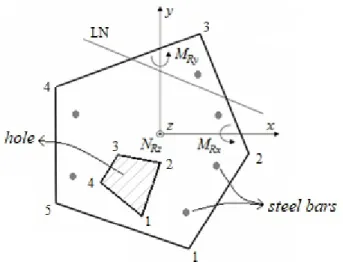
Identification of the polygonal section is done through the number of vertices and their plane coordinates, as shown in Figure 1. The steel bars are defined in a punctual shape in the interior of the section. Holes can be defined in the sec-tion. For the calculation of the resistance forces in the reinforced concrete polygonal section, a routine using Green's theorem will be used to transform the integral along the polygonal section area into an integral along its border (see ref. Sousa and Caldas (2005)). Thus, the section containing holes should be transformed into a single section with the verti-ces of the holes sequenced in a clockwise direction, while the vertiverti-ces of the external section should be sequenced in the counterclockwise direction.
Figure 1: Cross-Section Shape.
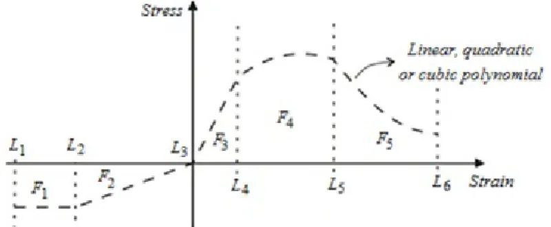
pre-sented herein. In this figure, Fi represents the deformation bands and Li the deformation limits of these bands. For each track, coefficients are defined that characterize the polynomial curve to be considered.
Figure 2: General shape of the stress-strain curve for the material.
2.2 Section deformation
In the definition of the equation for the cross-section deformation of a reinforced concrete linear element undergo-ing biaxial bendundergo-ing with axial force, the hypothesis for the plane section maintenance and perfect adherence between the concrete and the steel bars was were considered, ensuring a single deformation for the complete section. As such, the section deformation is given by Equation (1), where:
0 is the axial deformation in the origin of the reference system, while kx and ky are the curvatures in relation to the planes yz and xz, respectively. The local axis xyz can be observed in Figure 3.x
k
y
k
y
x
,
)
0
x
y(
(1)Figure 3: Flat shape of the cross-section deformation.
2.3 Resistance Forces
An imaginary cross-section in a bar element is subjected to the distribution of the normal stress when submitted to biaxial bending action with axial force. From the distribution of this stress, it is possible to determine the bending mo-ments MRx and MRy as well as the normal force NRz, which are defined as the resistance forces of the cross-section under analysis and obtained from Equations (2) and (4). In these equations, n is the number of steel bars in the cross-section, Asi is the area of n steel bars, xsi and ysi are the coordinates at the center of a steel bar, si is the normal stress on the cross-section at point xsi and ysi, and c is the normal stress on the cross-section at any one point in the section.
ni si si A c
Rz
dA
A
N
1
(2)
ni si si si A c
Ry
xdA
A
x
M
1
si n
i si si A c
Rx
ydA
A
y
M
1
(4)2.4 Objective function
In deterministic problems for structural optimization, the objective function is generally the volume or weight of the structure, and the constraints are related to the standard requirements code. In this study it is desired to obtain the mini-mum of the objective function given by Equation (5), where: n is the number of steel bars; Asi are the areas of n steel bars; and x is the set of the project variables presented in the following item.
ni
A
sif
1
)
(
x
(5)2.5 Project Variables
The project variables can be of two types: discrete or continuous. Variables of the first type can only assume integer values, while for the second type, can assume any real value within a determined interval.
Herein, the project variables (elements of the x vector shown in Equation 5) are all continuous being given by the areas of the steel bars and the parameters that define the section deformation; in other words, the axial deformation of the section and the curvatures of the section in the yz and xz planes.
Although these cannot of considered optimization variables, because they do not vary during the optimization pro-cess that involves the application of a sequential linear programming method in association with Simplex, the quantity of steel bars and their positions in the section can be considered variables of the problem because the steel bars configura-tion of the secconfigura-tion at the starting point could be different from that of the final secconfigura-tion obtained by the program (see Item 4).
2.6 Constraints
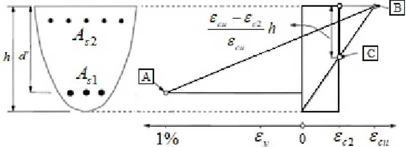
The constraints are conditions that should be satisfied for the project to be acceptable. For the design and detailing of any reinforced concrete polygonal section undergoing biaxial bending with axial force, the following constraints are defined: the compression strain limit of the concrete, the tension strain limit of the steel, and the resistance forces within the section should be greater or equal to the solicited forces. Other constraints that should be considered refer to the lat-eral ones for the steel bars diameter and step size of the linear approximation for the problem.
Concrete strain limits:
Figure 4 presents the possible strain distributions for a cross-section of a reinforced concrete linear element under-going biaxial bending with axial force in accordance with Eurocode 2 (2004) and ABNT NBR 6118 (2014). As seen in the figure, the longest fiber of the section should present a specific linear strain in an absolute value that is less than or equal to
cu (point B in Figure 4). In the case of a fully compressed section, the specific linear strain is an absolute valuefor the fiber positioned at
h
cuc cu
2of the longest fiber should be less than
c2 (point C in Figure 4). While the limitfor the linear specific strain at the points where the steel bars are should be less than 1% (point A in Figure 4).
Figure 4: Strain limits of the concrete and steel bars.
Figure 5. Considering that
tan
k
y/
k
x and Equation (6) for the section curvature, the Equation (7) for the defor-mation of the section is obtained.
k
xcos
k
ysin
(6)'
)'
,'
(
x
y
0
y
(7)Figure 5: Polygonal section and rotated reference system
For the x’y’ reference system, h1 is defined as being the coordinate y’ of the vertex of the polygonal section with the greatest y’ coordinate, while h2 is the y’ coordinate of the vertex with the least y’ coordinate. These vertices are high-lighted with a rectangle in Figure 5.
Defining h as being the distance between the vertices highlighted in Figure 5, or in other words, h = h1–h2, deter-mines the position of the points that are cu c2
cu h
of vertex h1 and vertex h2, data is obtained to be able to define the positions in the section of h3 and h4, respectively. With these definitions the Equations (8) to (11) for the constraints referring to the strain limits of the concrete are determined. In these equations,
cu and
c2 there are negative valuesthat refer to compression specific linear strain. In accordance with Eurocode 2 (2004) and ABNT NBR 6118 (2014) for concrete with
f
ck
50
MPa
, are defined
cu
0.35%
and
c2
0.2%
. For concrete withf
ck
50
MPa
, these concrete strain value depends on fck.cu
h
C
1(
x
)
0
1
(8)cu
h
C
2(
x
)
0
2
(9)2 3 0
3
(
)
h
cC
x
(10)2 4 0
4
(
)
h
cC
x
(11)Steel strain limits:
The Eurocode 2 and ABNT NBR 6118 code set the value of 1% for the tension strain limit at the points of the sec-tion where the steel bars are posisec-tioned. Thus, if (xi, yi) is a coordinate of the steel bar in the section, then:
0
)
,
(
01
.0
x
iy
i
. Defining h5 as being the y’ coordinate of the steel bar with the largest y’ coordinate, and h6 as being the y’ coordinate of the steel bar with the smallest y’ coordinate, as shown in Figure 5, the Equations (12) and (13) of the constraints for the deformation in the most solicited steel bar are obtained.)
(
01
,0
)
(
0 55
h
)
(
01
,0
)
(
0 66
h
C
x
(13)Soliciting forces:
In these study the section shown in Figure 1 can be submitted to biaxial bending with axial forces. The moment, which is obtained from the configuration of the analyzed steel bars configuration, Equations (3) and (4), should be great-er or equal to the soliciting moment (MSx and MSy). Equations (14) and (15) define the equations for the constraints refer-ring to the soliciting moment. In these equations, the resistance and soliciting moments are considered with their absolute values.
7 Rx Sx 0
C ( ) M - Mx (14)
8 Ry Sy 0
C ( ) Mx - M (15)
The axial force obtained from the steel bar configuration adopted, Equation (2), it should be equal to the normal so-liciting force (NS). Equation (16) shows this constraint of equality. In this text, the inequality constraints are elements of the C vector, while the equality constraints are elements of the D vector.
1( ) R S 0
D x N N (16)
As seen in Equations (14) to (16), the constraints for the soliciting forces are considered to be inequality for MRx and
MRy, and equality for NR. For most of the polygonal sections and steel bar configurations, these restrictions ensure the security of the section obtained in the analysis. However, there are sections with a certain steel bar configuration for which this is not true. For these sections, the inequality should be exchanged for equality constraints given by Equations (17) and (18). For example, the section with moment interaction curve shown in example 4 in the application of this paper, is safe for soliciting forces of Nd = 600kN, Mxd = 30kNm and Myd = 40kNm, but is unsafe when reducing Mxd of 10 kNm and the other soliciting forces are maintained. That is, a reduction of the soliciting moment made it unsafe, oth-erwise expected. At this point it is necessary to consider the moment constraint as being constraint of equality.
2 Rx Sx 0
D ( ) M - Mx (17)
3 Ry Sy 0
D ( ) Mx - M (18)
In the search method for the optimal point implemented in this study, starts from the point that satisfies all of the constraints, so that the constraints for the soliciting forces are attended under the condition of equality. During the itera-tive process for the definition of a new point that attends the constraints and reduces the objecitera-tive function, there was a tendency for all of the soliciting forces to remain equal to the resistance ones. If in one iteration of the method, a re-sistance moment was observed that began to stabilize at an absolute value greater than the soliciting moment, it was verified if the point (MRx, MRy) remained within the iteration curve of the moments for the analyzed section having a normal force (NR = NS). In case the situation remains, the inequality constraints are maintained in the following iterations of the algorithm for sequential linear programming. To the contrary, the constraint for the moment (or moments) ana-lyzed is transformed into an equality constraint for the following iterations of the algorithm.
Lateral constraints:
The lateral constraints are practical limitations for the variables of the project, i.e., a project variable referring to the dimension cannot be, in practice, less than zero or greater than a determined limit, setting as such the lateral constraints or barriers for a project variable. Within the project variables presented previously, the variables referring to the areas of the steel bars should have barriers, or in other words, they should have diameters less or equal to the diameter defined by the user and greater than zero, defining the constraints given by Equations (19) and (20). In these equations, A_s is the
area limit of the steel bars calculated from the diameter given by the user, and i = 1,2,...n with n being the number of steel bars.
0
i+8 si
C ( ) Ax (19)
0
_ i+n+8 s si
C ( ) A - Ax (20)
In the search method for the optimal point implemented in this study, sets the starting point
x
0 and obtain the next point that attends the project constraints and generates a reduction of the objective function from the iterative equation:k 1 k
se-quence of linear problems with the variables given by the vector
d
. In order to be valid the linear approximation used in the method implemented herein, it is necessary to impose lateral constraints for the step size, that is, d . In this way, we arrive at a set of constraints given below, where i varies from 1 until n+3, with n being the number of steel bars.Δ 0
i+2n+8 i i
C ( )d d (21)
Δ 0
i+3n+11 i i
C ( )d d (22)
3 OPTIMIZATION
Equation (23) below presents a general problem for optimization with equality and inequality constraints. In this equation, x is the vector for the project variables, f is the objective function to be minimized, C and D are functions of the project variables that define, respectively, the equality and inequality constraints of the problem.
)
(
min
x
x
f
subject to C ( )i x 0 e D ( )j x 0 (23)Herein, a sequential linear programming is used to analyze the non-linear problem studied. This method is quite simple and consists in the linearization of the objective and constraints function using the first-order Taylor series ap-proximations. Thus:
T
k k k
f(
x d
) f( )
x
f
d
, (24)T
k k
i i ik
C(
x d
) C( )
x
C
d
, e (25)T
k k
i i ik
D(
x d
) D( )
x
D
d
(26)In Equations (24) through (26),
Tf
k is a line vector with its terms given by the partial derivatives of the first or-der of the objective function in relation to the project variables being evaluated atx
k. Similarly,
TC
ik and
TD
ik are defined. Admitting that the starting point x0 is known which satisfies all of the project constraints, the problem consists in definingd
so thatf
(
x
k1)
is less thanf
(
x
k)
andx
k1 satisfying all of the constraints. Applying these conditions for the linear approximations of the objective function and constraints, the linear problem of Equation (27) for the defini-tion of stepd
for each iteration of the method is obtained.d
x k
Tf
min subject to
TC
ikd
C
i(
x
k)
e
TD
jkd
D
j(
x
k)
(27)The problem shown in Equation (27) presents objective functions and linear constraints in relationship with the var-iable defined by the terms of vector
d
. Thus, an optimization algorithm for linear problems can be used to determine stepd
in iteration k for the sequential linear programming method. Herein, the Simplex method is used for solving the prob-lem shown in Equation (27). In this method, the constraints and objective function should have linear relationships with the project variables, being as such called linear programming. The linear programming is started and analyzed in its standard form by Equation (28) below. In this equation, c and x are vectors in ℜs, b is a vector in ℜt and A is a matrix s xt, being s the number of project variables and t the number of equality constraints. x
c x
T
min subject to Axb,x0 (28)
* *d k 0 md
T k
Tf f
1
min
subject to
1 1 1 3 3 3 3 ) ( ) ( ] [ ] [ ] [ ] [ p k r q k m p n p T n pT m n m m
T n m T D C D D C C x x d* 0
I (29)
In Equation (29),
d
*
[
d
Td
Tu
T]
T, where d and d are two vectors with n+3 components (number ofpro-ject variables), u is a vector with m components (number of inequality constraints) called gap variables. Also, Imxm is an identity matrix of order m, and 0pxm is a null matrix with p lines and m columns, where p is the number of equality con-straints. Finally, q represents the number of inequality constraints excluding those referring to the step size so that q = m
– r, with r = 2n+6.
Equation (30) presents the partial derivatives of the objective function in relation to n+3 project variables, or, 1
1
A
sx
, ...,x
n
A
sn,x
n1
0,x
n2
k
x ex
n3
k
y. Meanwhile, Equations (31) to (38) present the partialde-rivatives of m inequality constraints in relationship to these project variables.
1, 1, ... 1, 0, 0, 0
T fk (30)
hi kx i khxi ky i khiy i
TC h h
(x) 0, 0, ... 0, 1 0 , , com i = 1,...,4 (31)
hi kx i khxi ky i khiy i
TC h h
(x) 0, 0, ... 0, 1 0 , , com i = 5 e 6 (32)
Rxy
x Rx Rx k M k M M sn sn s s s s
TC y y y
7(x) 1 1, 2 2, ... , 0 , , (33)
, , ... , , ,
,)
( 1 1 2 2 0
8 Ry xRy kRyy
M k M M sn sn s s s s
TC x x x
x (34)
8( ) 0 ... 0 1 0 ... 0
ção ésima posi i
i
TC x com i = 1,...,n (35)
8( ) 0 ... 0 1 0 ... 0
ção ésima posi i
n i
TC x com i = 1,...,n (36)
2 8( ) 0 ... 0 1 0 ... 0 ção
ésima posi i
n i
TC d com i = 1,...,n+3 (37)
3 11( ) 0 ... 0 1 0 ... 0 ção
ésima posi i
n i
TC d com i = 1,...,n+3 (38)
For the partial derivatives of the resistance forces and the section curvature in relation to 0 , kx and ky are presented below in Equations (39) and (44). In these derivatives Ec and Es are obtained from the derivative of the material stress-strain curve.
cos
sin
sec
cos
y
x y x k
k
k
k
2
,
sin
cos
2sin
sec
y x y k k y xk
k
k
2
, (39)
si n
i si si A
c
Rx E ydA A E y
M
1 0 , 2 1 2 si ni si si A c
x
Rx
E
y
dA
A
E
y
k
M
, (40)
si si n
i si si A
c y
Rx E xydA A E x y
k M
1, n si
i si si A
c
Ry
E
xdA
A
E
x
M
1 0si si n
i si si A
c x
Ry
E
xydA
A
E
x
y
k
M
1e 2
1 2
si n
i si si A
c y
Ry E x dA A E x
k M
. (42)
ni si si A
c
Rz
E
dA
A
E
N
1 0
, sin
i si si A
c x
Rz
E
ydA
A
E
y
k
N
1e (43)
si n
i si si A
c y
Rz
E
xdA
A
E
x
k
N
1. (44)
In Equations (31) and (32), the partial derivatives of hi (with i = 1,...,5) in relation to 0, kx and ky are determined using the finite differences method shown in Equation (45), where, ej is a vector with its terms being null, except the term in position j, that is equal to the unit.
j j j j j j Δx j
dx
f
dx
f
Δx
f
Δx
f
x
f
j)
(
)
(
)
(
)
(
lim
)
(
0x
e
x
x
e
x
x
(45)
Equations (46) to (48) present the derivatives of the equality constraints in relation to n+3 project variables. Being that Equations (47) and (48) present the derivatives of the constraints referring to the resistance moments when these are considered to be the equality constraints of the problem.
yR
x R R k N k N N sn s s TD 0 ... ) x
( 1 2
1
(46))
(
)
(
72
x
C
x
D
TT
(47))
(
)
(
83
x
C
x
D
TT
(48)4 ALGORITHM
Below is presented the algorithm for defining the amount of steel bars, their location in the section and their diame-ters so that the section meets the project constraints and utilizes a minimum amount of steel.
Step 1 – Define the cross-section, the material mechanical properties, the diameter of the steel bars, the soliciting forces (MSx, MSy e NSz), and
standard requirements to the detailing of reinforcement in the section, such as cover to bars and spacing between the steel bars.
Step 2 – Determine the starting point that meets all of the project constraints. This point is necessary to begin the iterative process for the search of the optimal point by using linear approximations for the constraints and objective function.
Definition of the starting point involves admitting values for the project variables so that the constraints are satis-fied. In case the user does not define the initial amount of steel bars and their positions in the section, a possible maxi-mum amount of steel bars in a layer on the contour of the section at the bars cover position is inserted. Verification of the need to utilize other layers of steel bars in the interior of the section is verified in the procedure describe in the following paragraph for defining the variables referring to the section’s deformation.
A routine was implemented that calculates the axial strain of the section and its curvatures in the xz and yz planes in such a way that the resistance forces would be equal to the soliciting forces. For this, an incremental process is used to-gether with the Newton-Rapson iterative method to solve this non-linear problem. As such, it was possible to set the variables referring to the section’s deformation or verify the need for inclusion of another layer of steel bars.
Step 3 – To obtain better behavior of the sequential linear programming method, an alteration of the section obtained in Step 2 was performed before applying Step 3, as described below.
Step 3.1 – Define m as the number of steel bars obtained in Step 2. In this step, all of the steel bars have the same diameter as defined by the user in the input file.
Step 3.2 – Calculate the derivatives of the resistance forces in relationship with each of the m steel bars. From the values encountered for the derivatives of each force in relation to a specific steel bar, their sum Sj is defined according to Equation (49). This equation is the
sensibility measurement for each of the steel bar, and can be used to verify which of the steel bars most influences the resistance forces and deformation of the section.
Ry Rx
R j
sj sj sj
M
M
N
S
A
A
A
Step 3.3 – Verify which of the steel bars has the smallest sum from the derivatives, or least Sj. Reduce the area of this steel bar in 25%. Other
reduction rates can be used. However, greater rates reduce the number of interactions in Step 3, but will result in a more super-estimated section in the following steps.
Step 3.4 – For steel bar configuration of the section obtained in the previous step, the parameters of the section deformation (0, kx and ky)
that generates resistance forces equal to the soliciting forces is calculated. For this, the routing described in Step 2 is used.
Step 3.5 – With the section deformation obtained in the previous step, the maximum concrete and steel strain values can be calculated, which is then compared with the limit values specified by standards. If these calculated strain are smaller than the limit strain, go back to Step 3.2 and continued the steel bars reduction process. If not, adopt the previous section from the one analyzed and go on to Step 4.
Step 4 – Apply an iterative method to maintain certain steel bars and remove others. As is described in the following steps, this method optimizes a new section at each iteration, being this new section obtained by maintaining the steel bars with the greatest area and removing the steel bars with null area.
Step 4.1 - Define k = m, where, k is a integer variable that controls the number of steel bars in the section for each iteration of Step 4, and m
is the number of steel bars obtained in Step 2.
Step 4.2 – Calculate the project variables that minimize the objective function f(x) respecting all of the constraints previously defined. In this step, a sequential linear programming method is applied together with the Simplex method to define new areas of steel bars that minimize the objective function.
Step 4.3 – The previous step alters the steel bars areas of the configuration being analyzed. As the steel bars diameter is limited by the diameter defined by the user, those steel bars that contribute in a more significant way to the resistance forces of the section tend to be amplified up to the diameter’s limit value. While the steel bars that least contributes to these forces, tends to reduce the diameter until its inferior limit. Therefore, in this step, the steel bars that have a diameter equal to the diameter supplied by the user, or very close to it, is maintained, and the steel bars that had their diameter zeroed, or very close to zero, is removed.
Step 4.4 – In the input file the user can choose if the steel bars should be of the same diameter, or if the same should only have a maximum diameter, i.e., being able to vary within the greatest and least commercial value determined. If the user choses steel bars of the same diameter do (i), else do (ii).
(i) Of the steel bars that were not excluded or maintained in Step 4.3, verify that which has the greatest area and set it for the diameter established by the user. Reduce k in accordance with the steel bars maintained and removed, and continue to Step 4.5. (ii) Of the steel bars were not excluded or maintained in Step 4.3, verify that it has the greatest area and fix it, defining for it the
greatest commercial diameter and the closest to this area, which is at most, the diameter defined by the user. Reduce k in accordance with the maintained and removed steel bars, and continue to Step 4.5.
Step 4.5 – In the input file, the user can choose if the steel bars should be placed in a symmetric manner in the section, or not. If symmetry is a requisite, it should be verified that the steel bar exists in symmetric positions for the steel bar fixed in Steps 4.3 and 4.4, if they exists, then these steel bars should be fixed with the same diameters as those fixed in Steps 4.3 and 4.4. If they do not exist, these bars will be included and fixed in these symmetrical positions.
Step 4.6 – If k > 0 return to Step 4.2 with a new configuration for the section and set the rest of the steel bars. To the contrary, end the iterative procedure with the optimal point given by the last steel bars configuration.
This algorithm works with discrete variables when it is fixing or removing steel bars, defining a new amount of steel bars, and defining the commercial diameter of the steel bars. The continuous variables appear in Step 4.2 when the areas of the cross-section of the steel bars are altered and the section is deformed to minimize the objective function.
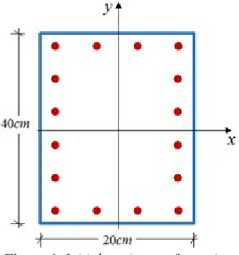
5 APPLICATIONS 5.1 Example 1
In this example, the least amount of steel for which a rectangular section of 20x30cm can resist the combined load of compression axial force of 120kN and a moment of 20kNm is determined. The axial force is acting on the geometric center of the section and the moment is acting on the x axis, putting tensile stress on the lower part of the rectangle, see Figure 6. For the material, the stress-strain curves are considered in accordance with ABNT NBR 6118 (2014), with fck = 25MPa and fy = 500MPa. This example is solved utilizing the equilibrium equations (50) and (51) for the rectangular section, and the program developed in this study.
Solving the problen using equilibrium equations:
Equations (50) and (51) represent the equilibrium of the forces and moments, respectively, for an imaginary section of a RC linear element undergoing axial bending with axial force. These equations were developed taking into considera-tion that the steel bars are concentrated at a point and that there is constant distribuconsidera-tion of the normal stress in the region of the concrete under compression. For this last consideration, in order to supply satisfactory results, the region under compression of the section is reduced to 20%.
1 1 2 2
0.68
d c x s s s s
F bd A A (50)
2
1 1
0.68
1 0.4
´
2
d c x x s s d
M
bd
A
d d
d h F
(51)rebar on the side undergoing traction. Also, σc is the stress in the most compression fiber of the concrete, σs1 is the stress on the rebar positioned on the side compression by Md, and σs2 is the stress on the rebar positioned on the side under traction. These stresses should present a negative value if the rebar is under traction. Continuing, d is the distance from the centroid of the rebar distribution As2 until the most compression fiber of the section. In this example, is considered a rebar formed by steel bars of 10mm distributed in only one layer with 3 cm to thickness of concrete cover, and as such, d
= h – 3.5cm., d' is the distance from the centroid of the rebar distribution As1 until the most compression fiber of the sec-tion, b and h are the width and height of the section, respectively, and x is the distance from the null strain until the most compression fiber, divided by d.
Searching for an optimal solution for the amount of steel to be used, the possibility of dimensioning the section con-sidering rebar only in the region undergoing traction by Md will be verified, thus, As1 is said to be null.
Adopting As1 0, Md 20kNm, d = 26.5cm, h = 0.3cm, b = 0.2cm e fcd = 25MPa/1.4, and admitting
c
.0
2
%
(c fcd) for the most compression fiber, the value of x= 0.217 is obtained from Equation (45). For this value of x, the neutral line cuts the section and As2 undergoes traction. Admitting
s2
yd (s2 fyd), Equation (44) results in an area of steel As2 = 0.45cm2. As the section deformation is on a plane the equation
s2
.3
608
c is obtained for217
.
0
x
. Therefore, if
c
.0
2
%
have
s2
0
.
72
%
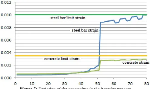
, which verifies the admissible conditions. analyzing the example using the implemented algorithm:In this example, a rebar cover of 3.0cm, spacing between bars of 3.0cm, and steel bars diameter of 10mm were con-sidered. Thus, in accordance with Step 2 of the algorithm presented in Item 4, the initial section is composed of 16 steel bars of 10mm, as shown in Figure 6. Also, the parameters of initial section deformation for which the resistance forces are equal to the soliciting forces are calculated in Step 2. The values 7
0 1.2610
, 3.90 10 -3
x
k and ky 0
were obtained from this Step 2. In Figure 7, it can be verified that for this deformation, the deformation constraints are met, and the starting point is x0.
Figure 6: Initial section configuration
After defining the starting point x0, alterations in the diameters of the steel bars are made, approximating the section for the optimal point of the problem, following the reasoning described in Step 3 of the algorithm presented in Item 4 herein. This approximation occurs until on the deformation limit constraints become very close to being violated. After-wards, the sequential linear programming method is used in conjunction with the Simplex method until the optimal point is defined as described in Step 4.2. At the end of this step, a section remains with only four steel bars in the underside face of the section with an area that is not null, totalizing an area of 0.46cm2. In this example, the final details of the section were not studied.
Figure 7: Variation of the constraints in the iterative process
As can be observed in this application, the response obtained using the equilibrium equations and the program im-plemented in this study is practically coincident. The small difference is due to the fact that in the imim-plemented program, the variation of the normal stress in the cross-section is represented according to the stress-strain relationship for con-crete defined by the standard Eurocode 2 (2004) and ABNT NBR 6118 (2014), while in the equilibrium equations, this variation is considered to be constant, reducing the area under compression to 20%.
5.2 Example 2
Bastos (2004) made a comparison of the design of reinforced concrete rectangular sections under biaxial bending with axial force by utilizing iteration abacus, and the design by using an optimization algorithm that had its formulation based on the genetic algorithm method. The problem proposed has a rectangular section of 40x60cm subject to a normal compression force Nd = 855kN and the soliciting moments Mxd = 490kNm and Myd = 230kNm. A distance of 2.5 cm from the center of the rebar to the section boundary was considered. The concrete and steel materials presented a stress-strain curve in accordance with standard (Eurocode 2, 2004, ABNT NBR 6118, 2014), with a yield stress (fy) for the steel of 420MPa and the compressive strength of concrete (fck) given by 25MPa.
The determination of the amount of steel required using the iterative abacus was done using the following parame-ters:
v
.0
2
, a 0.19, b 0.13 and
0
.
6
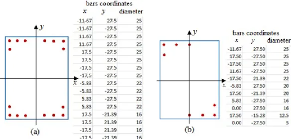
. Entering these parameters in the abacus, we have a rebar rate of 3.2%that should be uniformly distributed along the internal perimeter of the section. As such, the result is 16 steel bars of 25mm distributed within the section, totalizing a steel area of 78.54cm2. Figure 8-b demonstrates the section obtained using the abacus.
The optimal section obtained by Bastos (2004) when using a genetic algorithm is composed of 12 steel bars of 25mm and 8 steel bars of 10mm, for a total steel area of 65.19cm2, as shown in Figure 8-a.
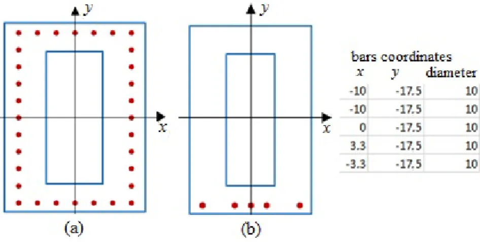
Figure 9 displays the configuration of the initial section defined by using the program implemented in this study. For this, it was considered that all of the steel bars had an initial diameter of 25mm and would be spaced 3cm apart. Therefore, the algorithm generates an initial section composed of 30 steel bars of 25mm, according to Figure 9.
Figure 9: Initial section obtained by algorithm proposed
Figure 10 presents the results obtained for the two analyses when considering the utilization of steel bars with a commercial diameter of 25mm or thinner and placed symmetrically in relation to the x and y axes for the first one, and unsymmetrically for the second one. The total steel area of the section was 62.52cm2 for the first analysis, and 35.16cm2 for the second one.
Figure 10: Section obtained in the (a) first and (b) second analysis using the algorithm proposed
5.3 Example 3
The problem proposed in this example involves a hollow rectangular section of 25x40cm and constant thickness of 6cm. The distance considered from the rebar center to the section external face was 2.5cm. The 10mm rebar was spaced at least 2.3cm apart from each other. The stress-strain curves for the steel and concrete materials were defined according to Eurocode 2 (2004). For the concrete, a parabolic-rectangular curve was adopted with fck = 25MPa,
c2
0
.
2
%
and%
35
.
0
cu
, and for the steel, perfectly plastic elastic curve was adopted with Es = 205GPa, fy = 420MPa, and%
1
su
.program generated 32 steel bar with a 10mm diameter, having a centroid distance of 2.5cm from the external boundary of the section, as shown in Figure 11-a. The user could exclude this option from the program and input the number of steel bars and their positions from the starting point.
Figure 11: (a) Initial section, (b) section obtained in the first analysis
In the first analysis bending only in the yz plane was considered, that is, N = My = 0 and Mx 50kNm. Symmetry of the rebar placements in relation to the y axis was required and all of the steel bars had a diameter of 10mm. With these specifications, the program converges for a section formed by 5 steel bars of 10mm, for a total steel area of 3.93cm2, as can be seen in Figure 11-b.
Figure 12: Section obtained in the (a) second, (b) third and (c) fourth analysis
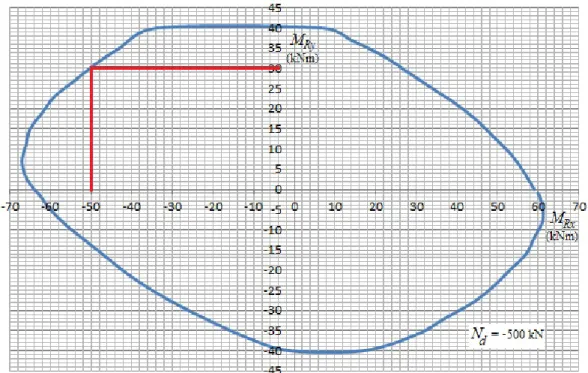
Figure 13: Moment interaction curve to section of the fourth analysis and Nd = -500kN
5.4 Example 4
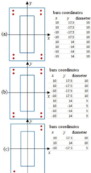
The problem proposed in this example is an L section with equal sides of 40 cm and a constant thickness of 12cm. The section is detailed with steel bars of 12.5mm considering a spacing of at least 2.3cm between each bar and a rebar cover of 2.0cm. The parameters that define the material are the same as those of the previous example. The section is submitted to biaxial bending with axial forces given by: Nd = -600kN, Mxd = 30kNm and Myd = 40kN. The forces are applied at the origin of the reference system shown in Figure 14-a of the initial section formed by 34 steel bars of 12.5mm with a centroid distance of 2.625cm from the external boundary of the section.
Figure 14: (a) Initial section, section obtained in the (b) first and (c) second analysis
Therefore, as in the previous example, Figure 15 shows the moment interaction curve of the section given in Figure 14-c for the compression axial force of 600kN. As can be verified by the curve, the points Mxd = 30kNm and Myd = 40kNm, are exactly within the boundary of this curve, indicating security and economy in the definition of this section.
6 CONCLUSIONS
In this study an optimization algorithm is presented to define the amount of steel bars, their diameter, and their posi-tion within any polygonal concrete secposi-tion undergoing biaxial bending with axial force, so that the amount of steel is the minimum needed to resist the soliciting forces. A sequential linear programming method is used to solve a non-linear problem for determining the resistance forces of the section in relationship with the project variables. In the iterative process of the sequential linear programming method the next step is determined so that the objective function has a maximum reduction, and to solve this problem was used the Simplex method. Some examples were analyzed to validate the proposed algorithm. The conclusions of these examples are presented in the applications section and briefly summa-rized below.
In Example 1 a rectangular section subjected to axial force and uniaxial bending in axis of symmetry was evaluated. In this way the solution of the minimum steel area can be obtained analytically. It was observed that the implemented algorithm obtained solution very close to the analytical solution.
In example 2 it is observed that the result obtained by the algorithm implemented in this study is practically the same result obtained from the literature. In this example the first-order algorithm of this study with a zero-order algo-rithm are compared in terms of results. Different from the algoalgo-rithm of this study that uses criterion derivatives, the ge-netic algorithm is a stochastic method that uses only the criterion value at some positions.
In examples 3 and 4 more complex polygonal sections were analyzed. For these sections no results were found in the literature for comparison. This is another contribution of this work. In these examples the validation of the imple-mented algorithm is done with the presentation of the initial section of analysis and the optimized section, and the check-ing of the solicitcheck-ing forces through the moment interaction curve for the optimized section. From this curve it is observed that for the soliciting axial force the ordered pair defined by the soliciting moments is on the curve indicating safe and economical section.
As can be seen from the examples presented, the method implemented herein was efficient enough to analyze vari-ous practical cases.
Acknowledgements
The authors would like to thank the Federal University of Ouro Preto (UFOP), the CNPq, and FAPEMIG, for their financial support.
References
ABNT NBR 6118 (2014) Projeto de Estrutura de Concerto - Procedimento. ABNT – Associação Brasileira de Normas Técnicas. Rio de Janeiro, Brasil, 2014. (in portuguese)
Anaut, D. O., Di Mauro, G.F., Suárez, J.A., DI Mauro, R. R. (2006) Optimal Configuration of Primary Distribution Nets.: Simplex Method. Information Tecnológica. 17: 85-92.
Balling, R.J. and Yao, X. (1997) Optimization of reinforced concrete frames, J. Struct. Eng., ASCE. 123: 193-202.
Bastos, E. A. (2004) Otimização de Seções Retangulares de Concreto Armado Submetidas à Flexo-Compressão Oblíqua Utilizando Algoritmos Genéticos. Dissertação de Mestrado, COPPE/UFRJ, Rio de Janeiro, RJ, Brasil. (in portuguese)
Bona, E., Borsato, D., Silva, R. S. S. F., Herrera, R. P. (2000) Aplicativo para Otimização Empregando o Método Sim-plex Sequencial. Acta Scientiarum. 22: 1201-1206.
Bonet, J. L., Barros, M. H. F. M., Romero, M. L. (2006) Comparative study of analytical and numerical algorithms for designing reinforced concrete sections under biaxial bending. Computers & Structures. 84: 2184–2193.
Camp, C.V., Pezeshk, S., and Hansson, H. (2003) Flexural design of reinforced concrete frames using a genetic algo-rithm, J. Struct. Eng., ASCE. 129: 105-115.
El-Tawil, S., Deierlein, G. G. (2001) Nonlinear analysis of mixed steel–concrete frames. II. Implementation and verifica-tion. J Struct Engng, ASCE. 127: 656-665.
Eurocode 2 (2004) European Committee for Standardization – EM 1992-1-1: Design of Concrete Structures – Part 1-1: General Rules for Buildings. Brussels: CEN. 225p.
Guerra, A., Kiousis, P. D. (2006) Design Optimization of Reinforced Concrete Structures. Computers and Concrete. 3: 313-334.
Haftka, R., Kamat, M. (1985) Elements of structural optimization. Martinus Nijhoff Publishers; Boston.
Hsu, C. T. T. (1985) Biaxially loaded L-shaped reinforced concrete columns. J Struct Engng, ASCE. 111: 2576-2629.
Junior, E. C. P. (2006) Otimizações de Seções de Concreto Armado, Programa de Pós-Graduação em Engenharia Mecânica, Universidade Federal de Santa Catarina, Flarianópolis, SC, Brasil. (in portuguese)
Lee, C., and Ahn, J. (2003) Flexural design of reinforced concrete frames by genetic algorithm. J. Struct. Eng., ASCE. 129: 762-774.
Maia, J. P. R. (2009) Otimização Estrutural: estudo e aplicações em problemas clássicos de vigas utilizando a ferramenta solver. Dissertação de Mestrado, Escola de Engenharia de São Carlos, Universidade de São Paulo, São Carlos, SP, Bra-sil. (in portuguese)
Moharrami, H., and Grierson, D. E. (1993) Computer-automated design of reinforced concrete framework. J. Struct. Eng., ASCE. 119: 2036-2058.
Munoz, P. R., Hsu, C. T. T. (1997) Biaxially loaded concrete-encased composite columns: design equation. J Struct Engng, ASCE. 123: 1576-1585.
Nocedal, J., Wright, S. J. (2006) Numerical Optimization. Second Edition, Springer-Verlag. New York - USA.
Ramos, H. O. C. (2011) Um Algoritmo para Otimização Restrita com Aproximação de Derivadas. Tese de Doutorado, Programa de Pós-Graduação em Engenharia da Universidade Federal do Rio de Janeiro, COPPE/UFRJ, Rio de Janeiro, RJ, Brasil. (in portuguese)
Rath, D. P., Ahlawat, A. S., Ramaswamy, A. (1999) Shape Optimization of RC Flexural Members. Journal structural Engineering. 125: 1439-1446.
Rodriguez, J. A., Aristizabal-Ochoa, J. D. (1999) Biaxial interaction diagrams for short RC columns of any cross-section. J Struct Engng, ASCE.125: 672-683
Sfakianakis, M. G. (2002) Biaxial bending with axial force of reinforced, composite and repaired concrete sections of arbitrary shape by fiber model and computer graphics. Advances in Engineering Software. 33: 227-242.
Sias, F. M. e Alves, E. C. (2014) Dimensionamento Ótimo de Pilares Circulares de Concreto Armado Segunda a NBR 6118:2014. Engenharia Estudo e Pesquisa, ABPE. 16: 34-42. (in portuguese)
Silva, A. R., Sousa jr, J. B. M., Neves F. A. (2010) Otimização do Perfil I de Aço de Vigas Mistas de Aço-Concreto com Interação Parcial, MECOM/CILAMCE, Buenos Aires. (in portuguese)
Silva, A. R., Sousa jr, J. B. M., Neves F. A. (2011) Optimization of Steel-Concrete Composite Beams With Partial Inter-action by Sequential Linear Programming. XXXII CILAMCE, Ouro Preto.
Sousa jr., J. B. M.; Caldas, R. B. (2005) Numerical analysis of composite steel-concrete columns of arbitrary cross sec-tion. Journal of Structural Engineering. 131: 1721-1730.
Sousa Jr., J. B. M., Silva, A. R. (2007)Nonlinear analysis of partially connected composite beams using interface ele-ments. Finite Elements in Analysis and Design. 43: 954–964.
Sousa Jr., J. B. M., Oliveira, C. E. M., Silva, A. R. (2010) Displacement-based nonlinear finite element analysis of com-posite beam columns with partial interaction. Journal of Constructional Steel Research. 66: 772-779.
Sousa Jr, J. B. M., Silva, A. R. (2010) Analytical and numerical analysis of multilayered beams with interlayer slip. En-gineering Structures. 32: 1671-1680.
Vanderplaats, G. (1984) Numerical optimization technique for engineering design - with applications. McGraw-Hill Book Company. New York.