Quasi-linear PCA: low order spline's approach to non-linear principal components

Quasi-Linear PCA: Low Order Spline’s Approach

to Non-Linear Principal Components

Nuno Lavado, Member, IAENG, and Teresa Calapez

Abstract—Nonlinear Principal Components Analysis (PCA) addresses the nonlinearity problem by relaxing the linear restrictions on standard PCA. A new approach on this subject is proposed in this paper, quasi-linear PCA. Basically, it recovers a spline based algorithm designed for categorical variables and introduces continuous variables into the framework without the need of a discretization process. By using low order spline transformations the algorithm is able to deal with nonlinear relationships between variables and report dimension reduction conclusions on the nonlinear transformed data as well as on the original data in a linear PCA fashion. The main advantages of this approach are; the user do not need to care about the discretization process; the relative distances within each vari-ables’ values are respected from the start without discretization losses of information; low order spline transformations allow recovering the relative distances and achieving piecewise PCA information on the original variables after optimization. An example applying our approach to real data is provided below.

Index Terms—nonlinear principal components analysis, quasi-linear PCA, linear PCA, CATPCA.

I. INTRODUCTION

A

the same basic premise and general objectives: the original data can be viewed as a collection of n points in some high (m-)dimensional space, the points correspond-ing to sample individuals and the dimensions to measured variables, and we seek for a suitable low (p-)dimensional approximation in which the points are positioned such that as much information as possible is retained from the original space. By reducing the dimensionality, one can interpret few components rather than a large number of variables.

Different interpretations of the phrase “as much informa-tion as possible” lead to the different multivariate techniques for dimension reduction.

One technique can be described as linear when the high-dimensional set of coordinates is replaced by another in a one-to-one linear relation with it. Principal Component Analysis (PCA) is probably the most common descriptive multivariate technique for seeking linear structure in data.

All attempts to generalize PCA in order to handle nonlin-ear structures, the generally denominated Nonlinnonlin-ear Principal Components Analysis, share the basic premise and general objectives mentioned, but they address the nonlinearity prob-lem by relaxing the linear restrictions between spaces.

Submitted March 23, 2011.

N. Lavado is with the Department of Physics and Mathematics, Coimbra Institute of Engineering (ISEC), Coimbra, Portugal and with the research unit Instituto Universit´ario de Lisboa (ISCTE-IUL), Unidade de Investigac¸˜ao em Desenvolvimento Empresarial (Unide-IUL), Lisboa, Portugal, e-mail: [email protected].

T. Calapez is with the research unit Instituto Universit´ario de Lisboa (ISCTE-IUL), Unidade de Investigac¸˜ao em Desenvolvimento Empresarial (Unide-IUL), Lisboa, Portugal, e-mail: [email protected].

The proposed approach was inspired by the Gifi system, also called Homogeneity Analysis, in particular by its natural successor: the work developed by the Data Theory Scaling System Group (Leiden), which introduced splines into the framework [1]–[3]. A brief review on splines is provided in Section II.

The existing Alternating Least Squares (ALS) algorithm for Homogeneity Analysis allowed an elegant embedding of least squares estimation of the spline coefficients resulting in a SPSS implementation called CATPCA (acronym for CATegorical Principal Components Analysis) [3]. A brief account of the Gifi system and CATPCA is given in Section III.

The major goal of the proposed approach is to recover the spline based algorithm CATPCA, designed for categorical variables, and to introduce continuous variables into the framework directly without the need of a discretization pro-cess. This approach is more precise with regard to quantita-tive continuous variables and provides a better approximation of a strictly nonlinear analysis, becoming a valid option to perform nonlinear PCA for those variables. The main results on the proposed algorithm are reported in Section IV.

An application of nonlinear PCA to an empirical data set (EuroStat economic indicators) that incorporates continuous variables and unknown nonlinear relationships between vari-ables is provided is Section V. The nonlinear PCA solution is compared with the linear PCA solution and with CATPCA solution on the same data. In the final section, we summarize the most important aspects of this approach, focusing on its strengths and limitations as an exploratory data analysis method.

II. SPLINE’S BRIEF REVIEW

Low order spline functions play an important roll in our quasi-linear PCA (qlPCA) proposal.

Basically, a spline is a piecewise polynomial function defined by a degree or order (degree plus one) and a set of interior knots. It can be shown [4], [5] that the set of splines of degree v with r interior knots is a linear space of functions, with dimension w = v + 1 + r, therefore equal to the spline’s order plus the number of interior knots. Spline application requires the use of a suitable set of

basis splines Bi, i = 1, . . . , w such that any piecewise

polynomial or spline f of degree v and associated with a determined knot sequence can be represented as the linear

combination f = ∑aiBi. In 1966, Curry and Schoenberg

have built a basis, using B-splines, which revealed to be especially convenient for computation when specified by recursion. They also derived a set of basis splines particularly

appealing to statisticians, the M-spline family in which Mi,

i = 1, . . . , w, is defined such that it has the normalization

∫

Monotone splines can be achieved by employing a basis

consisting of monotone splines Ii(x) =

∫x

−∞Mi(u)du [6].

This provides a set of splines which, when combined with

nonnegative values of the coefficients ai, yields monotone

splines. Because each Mi is a piecewise polynomial of

degree v, each Ii will be a piecewise polynomial of degree

v + 1.

As an illustrative example, if one wants to achieve a spline function of degree one with a interior knot it will be necessary in the first place to compute the set of two

M-splines basis functions of degree zero with one interior

knot. As these basis functions are piecewise polynomial of

degree zero, each Iiwill be a piecewise polynomial of degree

one as needed. Therefore this set of I-splines basis functions will have two elements. As the entire space of degree one spline functions with one interior knot is three-dimensional, the referred set can only generate one of its subspace.

Figure 1 displays the family of I-splines of order two defined on [0, 1] and associated with one interior knot at the median. Each I-spline is piecewise linear and nonzero over at most one interval.

min median max

0 0.2 0.4 0.6 0.8 1 1.2 1.4 1.6 1.8 2 original variable

recoded & transformed variable

I₁→

I2→

spline=1.2I

1+0.6I2→

Fig. 1. Spline of order 2 with one interior knot at the median. I1 and I2

are the basis spline functions. Stars represent the images of x through the

spline obtained as a linear combination of I1 and I2 with coefficients 1.2

and 0.6, respectively.

Figure 1 also displays an example of the images obtained by each of the three functions (two basis functions and one spline) for a value of x above the median (x = 0.58,

I1(0.58) = 1, I2(0.58) = 0.29 and spline(0.58) = 1.37).

A degree n polynomial is determined by n + 1 points. Therefore, each line segment from Figure 1 could be achieved only with the points associated with the mini-mum/median and median/maximum. However, during the optimization process of the spline transformation, the qlPCA algorithm will search for the optimal (as defined in the next section) linear combination of I-splines through a multiple

linear regression with I1 and I2 as predictor variables and

thus involving the whole data and not only those two points.

III. GIFI SYSTEM ANDCATPCA

For a comprehensive overview on the Gifi system see [7], a recent review is given by [8] and [2].

The central themes of the Gifi system are the notion of

optimal scaling and its implementation through alternating

least squares algorithms. The optimal scaling process as defined by the Gifi system is a transformation of variables

by assigning quantitative values to qualitative variables in order to optimize a fixed criterion. Optimality is a relative notion, however, because it is always obtained with respect to the particular data set that is analyzed. This process (optimal quantification, optimal scaling, optimal scoring) allows nonlinear transformations of the variables. Variable transformation has become an important tool in data analysis over the last decades. For an historical overview see [2].

One of the optimal scaling procedures for dimension re-duction and their SPSS implementation - CATPCA - was de-veloped by the Data Theory Scaling System Group (DTSS), consisting of members of the departments of Education and Psychology of the Faculty of Social and Behavioral Sciences at Leiden University.

The CATPCA algorithm is the state-of-the-art to perform nonlinear PCA for ordinal and nominal data [2]. CATPCA is available since 1999 from SPSS Categories 10.0 onwards [3]. The traditional crisp coding of the categorical variables was maintained and the least squares estimation of the spline coefficients is performed by a multivariate regression on each iteration of the ALS procedure. This approach performs very well with categorical variables, but it needs an a priori discretization process for quantitative variables or categorical not coded in the traditional way. And by so it is no longer precise with regard to quantitative variables. However it should be emphasized that Leiden’s solution emerge from psychometrics therefore, dealing mainly with categorical variables.

CATPCA procedure simultaneously quantifies m categor-ical variables while reducing the dimensionality of the data. Moreover, CATPCA, with respect to ordinary PCA, allows to treat variables not only as numeric, but as ordinal, nominal, spline ordinal or spline nominal as well. The technique

consists of finding object scores X of order n × p (i.e.

n = number of case-objects, p = number of dimensions)

and sets of multiple category quantifications Yj of order

kj× p (i.e. kj = number of categories of each variable and

j = 1, . . . , m) so that the loss function: σ(X, Y) = m−1∑ j tr [ (X− GjYj) ′ (X− GjYj) ] (1)

is minimal, under the normalization restriction X′X = nI,

where: Gj is an indicator matrix for variable j, of order

n× kj, whose elements are 0 when the i-th object is not in

the r-th category of variable j and 1 when the i-th object is

in the r-th category of variable j; I is the p× p identity

matrix. The algorithm uses Alternating Least Squares to minimize the loss function. It consists of two phases, a model estimation phase and an optimal scaling phase, iteratively alternated until convergence is reached. Both the component loadings and the category quantifications are changed until the optimum is found.

It should be emphasized that the optimum found is a relative one since it depends on class of admissible trans-formations. In what splines are concerned, each class of transformations depends on the number of knots, spline’s degree and knots placement. However, while the fitting problem is linear in the basis coefficients, it is highly nonlinear in the knots, and therefore it is desirable to avoid much optimization with respect to them [6]. The choice

of a particular spline could be targeted according to the percentage of explained variance, by trying different sets of parameters. However, like all statistical models, nonlinear PCA via splines is subject to overfitting when there are too many parameters in the model, which means in this context a high dimension linear space of splines in use. In order to prevent overfitting a reasonable number of data should be in the vicinity of any interior knot [6].

IV. QUASI-LINEARPCA

The indicator matrices introduced in the previous section are only used in the equations and of course not in the actual implementation of the CATPCA algorithm. However, the CATPCA algorithm was developed in the ’80’s initially as an algorithm for categorical data analysis, thus for dealing with integer valued variables. Regarding continuous data it needs to pass through a discretization process before the ALS algorithm starts. Various discretization options are available for recoding continuous data and one can always recode data outside CATPCA. The qlPCA approach is to adjust the algorithm to allow continuous values directly avoiding researchers in fields dealing with continuous variables to think that some information is being neglect.

The main advantages of this approach are: the user does not need to care about the discretization process; the relative distances within each variables’ values are respected from the start without discretization losses of information. Although one can think that this last aspect is irrelevant for nonlinear transformation, as the relative distances are going to be lost anyway, when the transformation is stepwise linear as in qlPCA this is not the case.

A. Optimal scaling revisited

Equation (1) can be re-written in a more general format

into the loss function σ : Mn×p×Mpm×n→IR so that

σ (X, Φ) = m−1∑ j tr [ (X− Φj(hj)) T (X− Φj(hj)) ] , (2)

under the normalization restriction XT_{X = nI where}

Φj =

[

ϕj1(hj) . . . ϕjp(hj)

]

is the n × p matrix

collecting the p (different) images of the (same) vector hj,

ϕjt the transformed variable j associated with dimension t,

t = 1, . . . , p and Φ =[ Φ1 . . . Φm

]T

is an pm× n

matrix.

Notice that the matrix Φj contains the images of the

same vector hj, subject to p different transformations. If no

restrictions are imposed upon the matrix Φj, then each value

of the jth _{variable receives p different quantifications, one}

for each dimension considered, in what is commonly called

Multiple quantification [3], [7], [9]. Having fixed the class

of admissible transformations for each variable, the purpose is to find the object scores and the quantifications that mini-mizes the loss function (2). The main differences between the existing algorithms to solve the loss minimization problem are within the class of admissible transformations. When those transformations are splines the following parameters must be defined: spline’s degree, number of knots and their placement.

Let ϕj be a spline of degree v with r interior knots,

spanned by w = v + r I-splines ϕj = ϕj(hj) = w ∑ i=1 αjiI [v] ji (hj) = w ∑ i=1 αjiI [v] ji = G△j yj, (3)

where: G△_j is the pseudo-indicator matrix for variable j, of

order n× w whose columns are the image vectors of the

variable j by each of the I-splines basis functions; yj is a

vector of length w whose elements are the linear combination coefficients yj= [α1α2. . . αw]

′ .

In the previous section the optimal scaling or optimal quantification process was defined within categorical analysis as the transformation of variables by assigning quantitative values to qualitative variables in order to optimize equation (1). Using equations (2) and (3) it is possible to re-define the optimal quantification process as a ALS phase that, given the

object scores optimize, the vectors yj in order to minimize

the loss function, or analogously, as the ALS phase that seeks to find the optimal linear combination for each basis spline given the object scores from the model estimation phase, therefore obtaining the optimal spline to transform each variable.

Notice that if the chosen class of admissible transforma-tions are splines of degree one without interior knots the ALS optimization of equation (2) yields the traditional (linear) PCA solution.

Usually, if the measurement level is ordinal, we may want to impose order restrictions, i.e, it is possible to change the values of each category but not the order between them. This means that the class of admissible spline transformation is limited to be a nondecreasing one. For quantitative variables, distance restrictions are usually also required, which can be imposed by the splines’ parameters (degree, number of interior knots and its placement). If there are reasons to believe that nonlinear relationships between variables exist, we may want to impose some other type of constraints to the transformed variable, also stated by the splines’ parameters. A familiar way to implement those ideas starts by

im-posing rank one to the matrix Φj, on what is usually called

Single quantification [3], [7], [9]. From a geometrical point of

view, in the case of two dimensions, Multiple quantification means that categories may lie anywhere in the space, whereas with Single quantification it is required that they fall on a straight line.

B. qlPCA algorithm

The qlPCA algorithm uses ALS to minimize (2) using

rank one matrices Φj. It consists of two phases iteratively

alternated until convergence is reached, a estimation of X phase and an optimal quantification phase by a multivariate regression having the spline basis functions as predictor variables on each iteration of the ALS procedure. So, qlPCA algorithm is very similar to CATPCA’s but it does not require integer variables as input.

The qlPCA algorithm will take advantage of low order splines, without limitation concerning the number of interior knots, in order to achieve nonlinear PCA as a straightfor-ward generalization of the traditional PCA solution and its measures of performance and interpretation.

Nonlinear PCA techniques usually report its solution with relational measures between the nonlinear transformed vari-ables obtained after the convergence test is reached and the associated objects scores.

Suppose, as an example, that CATPCA was performed and achieved 84% of variance explained using two dimensions

being the first nonlinear component loadings l1 = [0.76 −

0.88 0.014]. This means that the first two dimensions explain 84% of the total variance of the transformed variables

-not of the original ones. The first loading of l1 means that

there is a substantial positive linear correlation between the first nonlinear principal component and the first nonlinear transformed variable.

By considered low order splines some relations between nonlinear principal components and the original variables can be revealed.

Let’s consider that the class of admissible functions are splines of degree one with some interior knots (one, for presentation simplicity) and l1= [l11. . . l1m] the component loadings vector associated with the first nonlinear principal component: P C1= l11ϕ1+ . . . + l1mϕm. (4) By (3), l1jϕj= l1j w ∑ i=1 αjiI [v] ji, j = 1, . . . , m (5)

and when the number of interior knots is equal to one,

l1jϕj= l1jαj1I

[1]

j1 + l1jαj2I

[1]

j2. (6)

Although I-splines are obtained by recursion, their def-inition for this particular case is as follows; for an input

continuous variable x with minimum m1, median m2 and

maximum m3: I1(x) = { x m2, x≤ m2 1 c.c. I2(x) = { m2−x m2−m3, x > m2 0 c.c. . Therefore, l1jϕj=      l1jαj1 m2 x, x≤ m2 l1jαj1+ l1jαj2m2 m2−m3 − l1jαj2 m2−m3x x > m2 . (7)

It is now possible to report dimension reduction conclu-sions on the nonlinear transformed variables as well as on

the original variables. The loading l1j is the value of the

linear correlation coefficient between P C1 and the

trans-formed variable ϕj = ϕj(hj) whereas (

l1jαj1

m2 ,−

l1jαj2

m2−m3)

define the piecewise loadings between P C1 and the piece

of the original variable hj below and above the median,

respectively.

V. EUROSTAT DATA ON ECONOMIC INDICATORS

The proposed approach will be illustrated using twelve economic indicators from 26 european countries publicly available from EuroStat. Notice that this is a convenient il-lustration of our approach rather than a substantive economic application.

The selected indicators are described in Table 1 (check glossary at EuroStat website).

TABLE I

SELECTED ECONOMIC INDICATORS.

Variable Code

1. Balance of international trade in goods tec00044 2. Balance of international trade in services tec00045 3. Harmonized Indices of Consumer Prices teicp000 4. Harmonised unemployment rate teilm020 5. Long term government bond yields teimf050

6. GDP per capita in PPS tsieb010

7. Real GDP growth rate tsieb020

8. Expenditure on pensions tps00103

9. Balance of payments teibp070

10.Motorisation rate tsdpc340

11.Human resources in science and technology tsc00025

12. Public balance tsieb080

As shown on figure 2, although no order restrictions were imposed, all optimal spline transformations turn out to be monotonously increasing. −50 0 50 −5 0 5 −100 0 100 −5 0 5 100 120 140 −5 0 5 0 20 40 −5 0 5 0 10 20 −5 0 5 0 200 400 −5 0 5 −5 0 5 −5 0 5 5 10 15 −5 0 5 −5 0 5 x 104 −5 0 5 0 500 1000 −5 0 5 20 40 60 −5 0 5 −20 −10 0 −5 0 5

Fig. 2. Optimal transformation plots obtain with qlPCA for each variable.

Table two shows the summarized results obtained after applying the proposed algorithm (qlPCA), CATPCA (both with splines without order restrictions of degree one and one interior knot and choosing the multiplying discretization option for CATPCA) and PCA (ordinary PCA) over the data set. The fit is expressed in terms of percentage of explained variance by two dimensions.

TABLE II

EXPLAINED VARIANCE BY TWO DIMENSIONS.

Algorithm (%)

qlPCA 58

CATPCA 64

PCA 54

It can be observed that qlPCA and CATPCA performances are slightly better than the linear one. One can try to improve nonlinear performances by increasing the number of param-eters (see additional considerations on section III). Despite qlPCA underperforming CATPCA, it should be emphasized that the proposed algorithm is not intended to be a direct competitor of CATPCA but rather a different approach.

It is possible to propose an interpretation for the meaning of the principal components and understanding the relative

positioning of countries based on the loadings, similarly to linear PCA.

TABLE III

COMPONENT LOADINGS- quasi-linear PCA.

Variable PC1 PC2 V1 -0.63 0.37 V2 -0.02 -0.58 V3 0.76 -0.44 V4 0.62 0.40 V5 0.89 0.25 V6 -0.80 0.18 V7 -0.32 -0.61 V8 -0.45 0.55 V9 -0.18 -0.65 V10 -0.72 0.18 v11 -0.72 -0.21 V12 -0.63 -0.54

Shown In table 3 are the component loadings associated with the qlPCA solution. As a sample interpretation of the previous table, and without the pretension of presenting a substantive economic application, one can say that:

• countries with high positive scores on PC1 are

associ-ated with high long term government bond yields and low GDP per capita in PPS;

• countries with high absolute negative scores on PC1 are

associated with high per capita in PPS and low long term government bond yields;

• countries with high positive scores on PC2 are

associ-ated with high harmonised unemployment rate and low balance of payments;

• countries with high absolute negative scores on PC2

are associated with high balance of payments and low harmonised unemployment rate.

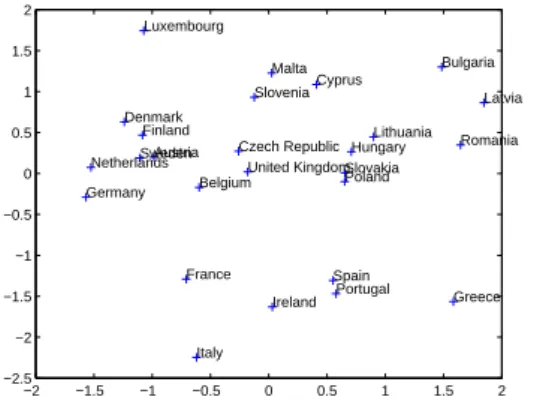
It should be noted that the previous conclusions on the original variables based on the nonlinear loadings are only possible because, as shown on figure 2, all transformations are monotone. If transformations turned out to be non-monotone similar interpretation were possible on the original variables’ pieces since transformations are based on degree one splines. −2 −1.5 −1 −0.5 0 0.5 1 1.5 2 −2.5 −2 −1.5 −1 −0.5 0 0.5 1 1.5 2 Italy Ireland Spain Portugal _Greece Poland Slovakia

HungaryLithuania Romania Latvia Bulgaria Cyprus Malta Slovenia Luxembourg Czech Republic United Kingdom Belgium France Austria Finland Denmark Sweden Netherlands Germany

Fig. 3. European countries projections on a 2-dimensional plot defined by the first 2 nonlinear principal components (qlPCA).

Figure 3 shows the projections defined by the first two

quasi-linear principal components on a two dimensional plot.

This chart can be a starting point for a clusters analysis, through visualization of potential groups of countries with

close projections. It is now possible to do some conclusions on countries’ indicators based, for example, on figure 3 extreme countries:

• Greece have high long term government bond yields,

low GDP per capita in PPS, high harmonised unem-ployment rate and low balance of payments;

• Bulgaria and Latvia have high long term government

bond yields, low GDP per capita in PPS but high bal-ance of payments and low harmonised unemployment rate;

• Luxembourg and Germany have high per capita in PPS

and low long term government bond.

VI. CONCLUSION

A new approach on Nonlinear Principal Components Anal-ysis (PCA) is proposed in this paper, quasi-linear PCA.

Basically, it recovers a spline based algorithm designed for categorical variables (CATPCA) and introduces contin-uous variables into the framework without the need for a discretization process. It should be emphasized that the proposed algorithm is not intended to be a direct competitor of CATPCA but rather a different approach.

By using low order spline transformations quasi-linear PCA is able to deal with nonlinear relationships between variables and report dimension reduction conclusions on the nonlinear transformed data as well as on the original data in a linear PCA fashion. The main advantages of this approach are: the user does not need to care about the discretization process; the relative distances within each variables’ values are respected from the start without discretization losses of information; low order spline transformations allow recov-ering the relative distances and achieving piecewise PCA information on the original variables after optimization.

Nonlinear PCA’s most known approaches among re-searchers dealing with continuous variables are autoassocia-tive neural networks, principal curves and manifolds, kernel approaches or the combination of these [10]. Therefore, comparisons studies with qlPCA will be taken.

REFERENCES

[1] J. Meulman et al., Optimal scaling methods for multivariate categorical

data analysis, SPSS white paper, SPSS Inc., 1998.

[2] J. Meulman, A. Kooij and W. Heiser, “Principal Components Analysis with Nonlinear Optimal Scaling Transformations for Ordinal and Nom-inal Data,” in The Sage Handbook of Quantitative Methodology for the

Social Sciences 2004, pp. 49-70.

[3] J. Meulman and W. Heiser, SPSS Categories 17.0, SPSS Inc.,2007. [4] C. de Boor, A Practical Guide to Splines, Springer, 1978. [5] L. Schumaker, Spline Functions: Basic Theory, Wiley, 1981. [6] S. Winsberg and J. Ramsay, “Monotone spline transformations for

dimension reduction,” Psychometrika, vol. 48, pp. 575-595, 1983. [7] A. Gifi, Nonlinear Multivariate Analysis, Wiley, 1991.

[8] G. Michailidis and J. De Leeuw, “The GIFI system of descriptive multivariate analysis,” Statist. Sci., vol. 13, pp. 307-336, 1998. [9] J. De Leeuw and J. Van Rijckevorsel, “Beyond Homogeneity Analysis,”

in: Component and Correspondence Analysis: Dimension Reduction by

Functional Approximation 1988, pp. 55-80.

[10] U. Kruger, J. Zhang and Lei Xie, “Developments and Applications of Nonlinear Principal Component Analysis a Review,” in: Principal

Manifolds for Data Visualization and Dimension Reduction 2007, pp.