Abstract — This paper presents an encoding scheme adapted for Fiber Bragg Grating (FBG) optimization using metaheuristics. The proposed encoding scheme uses spline approximations in order to build softened refractive index profiles from few encoded parameters. This approach is suitable for Fiber Bragg Grating (FBG) synthesis because it ensures both the reduction of the problem dimensionality and the respect of important restrictions associated to the FBG manufacture. Simulations are shown where an ES using the spline encoding was able to converge faster and produce more interesting filters, when compared with conventional encoding schemes.
Index Terms —FBG, Evolution Strategies, spline, chromosome, encoding.
I. INTRODUCTION
Fiber Bragg Gratings (FBGs) are flexible components. By adjusting the parameters that describes
their refractive index profile, it is possible to obtain filters showing reflectance spectrum adapted to
almost any type of application. Unfortunately, this procedure (FBG synthesis) is not a trivial problem
and several techniques have been proposed with some degree of success.
For example, if only weak gratings are considered, the refractive index profile can be obtained from
the Fourier Transform of the reflection coefficient. This was the approach used by Winick and Roman
[1] with interesting but inaccurate results. On the other hand, other techniques like these based on
Layer Peeling (LP) [2] [3] are capable of very accurate solutions in terms of reflectance spectrum, but
have as side effect the generation of large and complex refractive index profiles that are difficult to
built using Ultra Violet (UV) mask manufacture techniques [4]. In order to attend all restrictions
associated to the FBG manufacture, Askanes et al [5] proposed a hybrid method that combines
classical optimization techniques and the LP algorithm.
Other interesting design alternatives are those based on Evolutionary Algorithms (EA). Genetic
Algorithm (GA) [6] and Particle Swarm Optimization (PSO) [7] allow achieving satisfactory results
even under heavy restrictions imposed by the manufacture process. For example, in [8], a pioneer
article about the use of GAs for FBG synthesis, feasible Wavelength Division Multiplexing (WDM)
filters with negligible dispersion are obtained. In [9], the FBG synthesis is performed using the
Covariance Matrix Adapted Evolution Strategy (CMAES) with relative great success. Similar results
are achieved in [10] using PSO. In [11], a GA is applied in the synthesis of Triangular FBGs
(TFBGs). In [12], the TFBG synthesis is performed again, but using the CMAES.
FBG Optimization Using Spline Encoded
Evolution Strategy
M. J. de Sousa, J. C. W. A. Costa, R. M. de Souza, R. V. M. P. Pantoja
Although literature shows that metaheuristics can be used to synthesize FBGs, they suffer because
of the high number of parameters needed to represent a FBG properly. Using the modeling based on
uniform sections presented in [13], an apodized FBG one centimeter long could be well represented
by about one hundred uniform sections, each one modeled by four parameters. Even considering a
single parameter by section, about one hundred in total must be used to represent the entire FBG. This
high dimensionality can make the metaheuristic optimization scheme not practical. Frequently in the
literature a FBG is designed using a reduced number of uniform sections. For example, in [10], only
20 sections are considered. The use of a reduced number of sections can generate mismatches large
enough to work like mirrors inside the FBG, which can create several cavities along the grating. In
this case the reflectance spectrum can result noisy and full of undesired lobes, affecting the
metaheuristic convergence.
Therefore, it is interesting to produce softened refractive index profiles and find a way to do that
using as few parameters as possible. Fortunately, according to the information theory, softened signal
formats shall carry naturally less information and, consequently, it is possible to use less parameter to
encode them. This article explores the use of spline approximations to create softened profiles from
few points stored in ES individuals (chromosomes) [14]-[16]. Section II presents the basic FBG
model. Section III presents the usual way to encode a FBG and the proposed spline encodings.
Section IV presents the ES algorithm. Section V compares the performance of several encoding
schemes through computer simulations. Finally, Section VI presents the conclusions.
II. FBGMODEL
Following the matrix formulation from [13], the refractive index profile is given in function of the
axial distance z:
4
( ) eff cos eff
B n
n z n δn π z
λ
= +
, (1)
where neff is the effective refractive index, δn the modulation parameter and λB is Bragg wavelength.
Using the coupled mode theory, it is possible to calculate a 2x2 matrix F that represents a uniform
section of length ∆z:
( ) (0)
( ) (0)
R z R
S z S
∆
= ×
∆
F , (2)
where R(z) and S(z) stand for the field amplitude functions of the propagating and back propagating
modes respectively. Hence, R(0) and S(0) represent the field amplitudes before the section at z = 0
and, at z = ∆z, R(∆z) and S(∆z) represent the field amplitudes after the section. The transfer matrix F is
calculated in function of δn, λB, ∆z, and neff, all of them considered constant along the section. Indeed,
A non uniform Bragg Grating can be modeled as a sequence of M uniform short gratings (uniform
sections). Let Fk be the transfer matrix of the k-th section, where k = 0 for the first section at z = 0.
The total transfer matrix for the apodized grating of length L = M × ∆z can be obtained by multiplying
all its M section matrices:
1 2... 1... 1 0
T = M− × M− × k× k− × ×
F F F F F F F . (3)
Now (2) can be rewritten in function of the total matrix FT:
11 12
21 22
( ) (0) (0)
( ) (0) (0)
T T
T
T T
F F
R L R R
S L S F F S
= × = ×
F , (4)
where R(L) and S(L) represent respectively the field amplitudes of the propagating and back
propagating modes at z = L.
The FBG reflectance is given in function of FT elements by:
21
22
2
T
T F R
F
=
(5)
An apodized FBG can be represented in a vector form like ( δn0, δn1,…, δnk,…, δnM–2, δnM–1,λB 0, λB 1, …, λB k, …, λB M–2,λB M–1, ∆z0, ∆z1,…, ∆zk, ∆z M–2, ∆z M–1), which is also a natural way to represent a FBG as
an individual in metaheuristics. In practical terms, not all parameters should be present in the vector
because they could be constant or known for the entire grating. For example, the representation in the
format ( δn0, δn1, …, δnk–1, δnk, δnk+1, …, δnM–2, δnM–1 ) was essentially the way chosen in [12] to represent individuals in the CMAES.
III. ENCODING STRATEGIES
Let us consider to be enough to represent ES individuals as Y = ( y0, y1, …, yk–1, yk, yk+1, …, yM–2,
yM–1 ), where yk could be any parameter among δnk, λB k or ∆zk. This encoding scheme will be referred here as direct encoding (DE), where the number of search space dimensions is equal to M, the same
number of uniform sections. Satisfactory FBG representations make use of at least 20 sections for a
centimeter long grating [10]-[12].
An interesting way to reduce the number of dimensions is through some sort of indirect encoding,
where the individuals store few parameters in a vector form like X = ( x0, x1, …, xj–1, xj, xj+1, …, xm–2,
xm–1 ) with m < M. Any yk can be calculated from X using linear interpolation:
( )( )
k j j j k
y =x + x −x d − j (6)
where
1 k
m k d
M
× =
− (7)
encoding scheme given by (6) and (7) will be referred as linear encoding or LE.
Another approach is to replace the linear interpolation by a spline approximation. This paper
explores quadratic and cubic splines [16]. For the quadratic spline encoding (QSE), yk can be
calculated from X by
1
1 1
2 2
1 1
( )[ floor( )], 0
( )[ floor( )], 1
0.5[(1 ) ] [ (1 ) 0.5] , otherwise
j j j k k
k j j j k k
j j j
x x x d d j
y x x x d d j m
t x t x t t x
+ − − − + + − − = = + − − = − − + + − +
(8)
where dk is given by (7), j = round(dk) and t = dk – j + ½. The function round( ) returns the nearest
integer from the argument.
For the cubic spline encoding (CSE), the relationship between yk and X is given by:
3 2 2 3
(1 ) 3 (1 ) 3 (1 )
k
y =A −t + Bt −t + Ct −t +Dt (9)
where dk is given by (7), j = trunc(dk) and t = dk – j. The parameters A, B, C and D are given
respectively by:
1
1 1
6 4 , 0 ( 1)
, otherwise
j j j
j
x x x j m
A x
− +
+ + < < −
=
, (10)
(
)
1
1
3 2 , ( 1)
, otherwise
j j
j
x x j m
B x
+
+ < −
=
, (11)
(
)
1
1 3
1,
2 , ( 1)
otherwise
j j
m
x x j m
C x
+
−
+ < −
=
,
(12)
and
(
)
1 1 2 6 14 , 3
, otherwise
j j j
m
x x x j m
D x
+ +
−
+ + < −
=
. (13)
For m < 3 the cubic spline approximation shall be replaced by linear interpolation and yk shall be
calculated using (6) and (7).
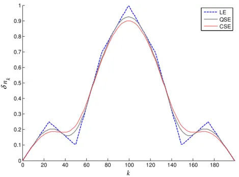
Examples of curves constructed by using LE, QSE and CSE are shown in the Fig. 1. The vector
(0.0, 0.25, 0.1, 0.7, 1.0, 0.7, 0.1, 0.25, 0.0) with m = 9 was used to produce these curves, each one
with 200 points (M = 200). As one can see, the spline approximations are smoother than LE and the
CSE is the most.
IV. EVOLUTION STRATEGY
Evolution Strategies, among other meta-heuristics like GA, evolve individuals applying nature
each generation [17]. Modern versions of ES use a population of parents and differ from GA basically
in the encoding and selection schemes [18].
0 20 40 60 80 100 120 140 160 180
0 0.1 0.2 0.3 0.4 0.5 0.6 0.7 0.8 0.9 1
k
δ n
k
LE QSE CSE
Fig. 1.δnkprofiles calculated using LE, QSE and CSE for M = 200, obtained from a test curve with m = 9.
Fig. 2. ES algorithm.
The adapted version of ES used in this article should be better defined as a (SA, SB) – ES, where SA
and SB are respectively the sizes of parent and child populations [19]. The algorithm is shown in Fig.
2. It starts creating two populations, A and B, to store respectively SA and SB individuals. Inside the
generation loop (line 5), each individual of B is replaced by a new one made by the application of the
01. Start A with SA random individuals;
02. Start B with SB (SB > SA) individuals;
03. Calculate the fitness for all individuals of A;
04. Store the A best individual in Abest;
05. For each generation:
06. For each B individual from B:
07. Select a random individual A1 from A;
08. B = A1;
09. If r < Aga( A1, PC) :
10. Select a random individual A2 from A;
11. B = Crossover( A1, A2 );
12. B = Mutation( B, Aga( A1, δ ) );
13. Calculate the fitness of population B;
14. Replace A by SA best individuals from B;
15. If Abest worse than A best:
16. Update Abest;
17. If Abest better than A best
intermediate crossover and Gaussian mutation. r in line 9 represents a uniform random value between
0 and 1. In this same line the function Aga( ) returns the crossover probability based on A1 rank, using
Adaptive Genetic Algorithm (AGA) procedure defined in [20]. Thus, the intermediate crossover
operator is optionally applied in line 11 using A1 and A2 (A2 ≠ A1) as parents. In line 12 the Aga( )
function is used again in order to feed Gaussian mutation with its standard deviation [18]. In the line
14 all individuals of population A are replaced by the SA best individuals copied from B. The iteration
is complete after the elitist procedure from 15 to 18. Note in the line 18 the individual Abest being
inserted in A, what set the population size temporally to SA + 1 until A be reset in line 14 in the next
generation. The fitness calculations in lines 3 and 13 are based on the sum of squared errors between a
target curve and the FBG reflectance spectrum. Let Ri be the i-th reflectance value calculated for
wavelength λi and Ti be the respective target value. The fitness value f for each individual can be calculated by
1
2
0
( )
N
i i i
f R T
−
=
=
∑
− , (14)where N represents the number of samples used to build the reflectance curve and Ri is calculated
using (5). Since the fitness function is an error value, the ES of Fig. 2 minimizes f.
The Aga( ) function used in lines 9 and 12 can be defined as
rank( )
, rank( ) Aga( , )
, otherwise
A
A h
A
α
α
hα
<
=
, (15)
where rank(A) returns the rank of the A individual inside population A (it returns zero for the best and
(SA – 1) for the worst), h is the rank of the individual whose fitness value is closest to the average, αis
the control parameter. Aga( ) returns zero for the best ranked individual in the population and α for
the worst.
V. SIMULATIONS
In order to validate the proposed encoding schemes, the ES defined in the previous section was
applied using direct encoding, LE, QSE and CSE. All following results were obtained using SA = 10,
SB =40, mutation deviation and crossover probability given by AGA using α equals to 0.01 and 1.0
respectively. The maximum number of generations of 10000 was used as stop criteria.
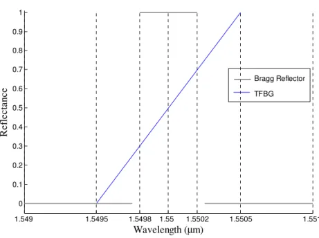
Two projects were used to compare the proposed techniques. The first one was a FBG centered in
1.55µm and the second was a TFBG from 1.5495µm to 1.5505µm. The target curves of both are
shown in Fig. 3. Note that the target curve for the FBG is not continuous. The interval from 1.5498µm
to 1.5502µm has two gaps of 0.05nm left and right. They offer accommodation space for reflectance
curves once abrupt targets are very difficult to fit.
Samples are spaced uniformly in terms of wavelength inside the target region. If one sample drops
inside a gap in the FBG target, it is not considered in the sum of (14). In all simulations the number of
uniform sections used was 50 (M = 50).
For each project and for each encoding, the ES was tested 20 times with different random initial
populations.
1.549 1.5495 1.5498 1.55 1.5502 1.5505 1.551 0
0.1 0.2 0.3 0.4 0.5 0.6 0.7 0.8 0.9 1
Wavelength (µm)
R
ef
le
c
ta
n
c
e
Bragg Reflector
TFBG
Fig. 1. Target curves for FBG and TFBG projects.
A. FBG project
For the FBG project, all sections have the same parameters ∆z and λB respectively set to 200µm and
1.55µm. Indirect encoding schemes used m = 5 for δn. Both direct and indirect encodings used 0 < δnk
<5×10⁻⁴.
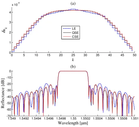
Fig. 3 compares the δn profile and reflectance curve for the most ranked Bragg reflectors
synthesized using LE, QSE and CSE. The linear interpolation was the worst among all indirect
encoding schemes. QSE and CSE schemes gave almost same results. Fig. 4 compares the results
obtained for QSE and DE. Direct encoding achieved the best reflectance curve, but the δn obtained
profile was not as smooth as others obtained using QSE and CSE. It is interesting to observe how all
profiles are near each other.
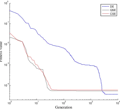
Fig. 5 shows the average evolution of fitness in function of generation number for ES using DE,
QSE and CSE. Direct encoding has poor performance since spends more generations to reach
convergence. This behavior was expected because here DE dealt with 10 times more dimensions in
search space than indirect encodings. The number of generations can be used safely as performance
measurement parameter because the fitness function is called exactly 40 times each generation.
negligible next the processing time spent in fitness calculations.
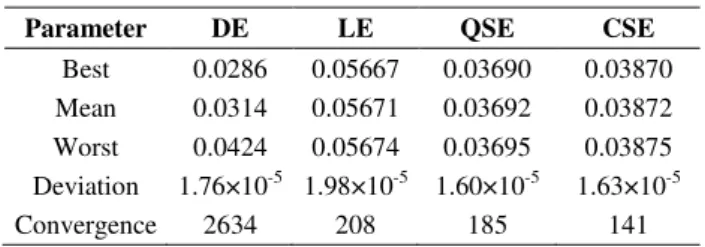
Table I shows performance parameters: the best final fitness found in all 20 runs, worst fitness
found, the mean fitness and the standard deviation. It also shows the convergence number, i.e., the
average number of generations necessary to grant fitness value with an error of 0.1% in comparison to
the last fitness value.
0 5 10 15 20 25 30 35 40 45 50
0 1 2 3 4
x 10-4
k
δn
k
(a)
1.549 1.5492 1.5494 1.5496 1.5498 1.55 1.5502 1.5504 1.5506 1.5508 1.551 -70
-60 -50 -40 -30 -20 -10 0
Wavelength [µm]
R
ef
le
ct
an
c
e
[d
B
]
(b) LE QSE CSE
0 5 10 15 20 25 30 35 40 45 50 0
1 2 3 4 5 6x 10
-4
k
δn
k
(a)
1.549 1.5492 1.5494 1.5496 1.5498 1.55 1.5502 1.5504 1.5506 1.5508 1.551 -70
-60 -50 -40 -30 -20 -10 0
Wavelength [µm]
R
e
fl
e
ct
an
ce
[
d
B
]
(b) DE QSE
Fig. 3. δn profiles (a) and reflectance spectrum (b) for FBG synthesized using QSE and DE.
100 101 102 103 104
10-4 10-3 10-2 10-1 100
Generation
F
it
n
e
ss
v
a
lu
e
DE QSE CSE
TABLE I. FBG PERFORMANCE PARAMETERS
Parameter DE LE QSE CSE
Best 0.0286 0.05667 0.03690 0.03870 Mean 0.0314 0.05671 0.03692 0.03872 Worst 0.0424 0.05674 0.03695 0.03875 Deviation 1.76×10⁻⁵ 1.98×10⁻⁵ 1.60×10⁻⁵ 1.63×10⁻⁵ Convergence 2634 208 185 141
B. TFBG project
For the TFBG project, all sections used ∆z = 400µm and linear chirp defined by the variation of λB
in function of k. As stated in [12], the linear chirp is necessary in order to achieve the desired
bandwidth of 1nm. However, differently from [12], where the linear chirp was fixed, here it was
defined by ES itself by encoding λB k in individuals always using LE with m = 2. The parameter δnk
was encoded using m = 7 for indirect encoding schemes. Thus, individuals were represented as a
vector of 9 dimensions for indirect encoding schemes and of 52 dimensions for DE. All encoded
schemes used 0 < δnk <5×10
-4
and 1549nm < λB k < 1551nm.
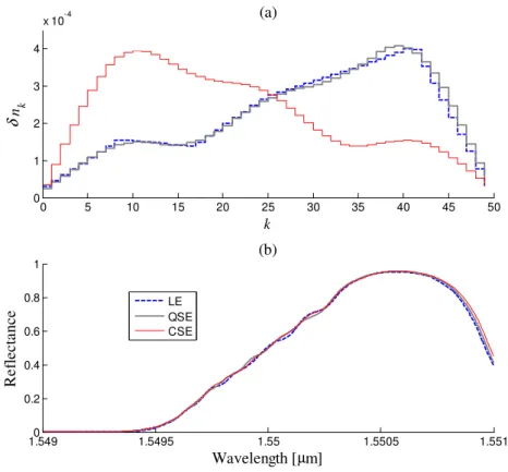
Fig. 7 compares δn profiles and reflectance spectra of best ranked FBGs synthesized using LE, QSE
and CSE schemes for the TFBG project. Fig. 8 compares only the results obtained by using QSE and
DE encodings. As observed in the Bragg reflector project, the linear interpolation brings the worst
results among all studied indirect encoding schemes. QSE and CSE are very similar to each other in
terms of reflectance but inverted in terms of profile. Indeed, the chirp obtained for DE, LE, QSE and
CSE were respectively 1.1536nm/cm, 1.4206nm/cm, 1.4254nm/cm and −1.4188nm/cm. The CSE
minus signal indicates a decreasing λB k toward the last section of the FBG. Since no restrictions were
imposed concerning the inclination of λB k curves, negative and positive values were obtained evenly
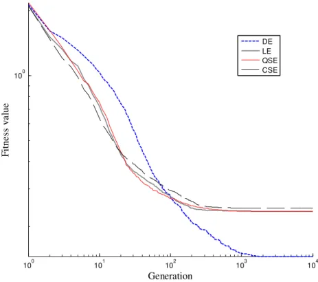
for all encodings. Fig. 9 shows the average evolution of the fitness value in function of generation
number for ES using direct encoding, LE, QSE and CSE. Table II shows some performance
parameters for TFBG project. As observed in the FBG project, the DE resulted again the best among
all encoding schemes in terms of fitness function. The DE superiority is not so obvious in terms of
reflectance as one can see in Fig. 8. As expected, the optimization process using DE spends more
generations to converge. However the difference between DE and indirect encodings is not so deep as
0 5 10 15 20 25 30 35 40 45 50 0
1 2 3 4
x 10-4
k
δ n
k
(a)
1.5490 1.5495 1.55 1.5505 1.551
0.2 0.4 0.6 0.8 1
Wavelength [µm]
R
e
fl
ec
ta
n
ce
(b)
LE QSE CSE
Fig. 7.δn profiles (a) and reflectance spectrum (b) for TFBG synthesized using LE, QSE and CSE.
0 5 10 15 20 25 30 35 40 45 50
0 1 2 3 4 5x 10
-4
k
δn
k
(a)
1.5490 1.5495 1.55 1.5505 1.551
0.2 0.4 0.6 0.8 1
Wavelength [µm]
R
ef
le
c
ta
n
c
e
(b)
DE QSE
100 101 102 103 104 100
Generation
F
it
n
e
ss
v
a
lu
e
DE LE QSE CSE
Fig. 9. Average curves of fitness value in function of generation number for DE, LE, QSE and CSE.
TABLE II. TFBG PERFORMANCE PARAMETERS
Parameter DE LE QSE CSE
Best 0.1218 0.1425 0.1326 0.1339 Mean 0.1456 0.2356 0.2354 0.2454 Worst 0.2035 0.2585 0.2723 0.3130 Deviation 0.0179 0.0396 0.0597 0.0642 Convergence 872 513 572 492
VI. CONCLUSIONS
Spline encodings combined to a modified evolutionary strategy have been successfully applied in
the FBG synthesis. Two projects have been considered and comparisons involving quadratic and
cubic spline encodings, direct encoding, and linear encoding have been provided. It has been shown
that spline schemes are able to reduce the number of dimensions and generate attractive softened
refractive index profiles.
Quadratic spline encoding (QSE) should always be considered in detriment of cubic encoding
(CSE) because it is simpler, has comparable performance and give better results.
However, spline encodings are not free of issues. If the search space is too much simplified, the
possible solutions can lose its flexibility. As result, the direct encoding overcame the indirect
profiles. An interesting possibility to conciliate performance and flexibility would be to use spline
encoding to achieve an initial solution for further application of a direct encoded meta-heuristic or
another suitable optimization technique.
The definition of m parameter in indirect encodings was accomplished based on a trial and error
procedure. A better way to do that could be through a progressive spline encoding scheme where the
number of parameters m would be increased gradually whenever the population diversity drops below
a threshold. This technique would require the insertion of new random parameters in individuals in
the middle of optimization process, probably in a very similar way as performed in [21].
REFERENCES