UNIVERSITAT DE BARCELONA
UNIVERSITY OF BARCELONA
FACULTAT DE QUÍMICA
FACULTY OF CHEMISTRY
D
D
e
e
v
v
e
e
l
l
o
o
p
p
m
m
e
e
n
n
t
t
a
a
n
n
d
d
A
A
p
p
p
p
l
l
i
i
c
c
a
a
t
t
i
i
o
o
n
n
o
o
f
f
Q
Q
u
u
a
a
l
l
i
i
t
t
y
y
S
S
t
t
a
a
n
n
d
d
a
a
r
r
d
d
P
P
r
r
o
o
c
c
e
e
d
d
u
u
r
r
e
e
s
s
(
(
O
O
p
p
e
e
r
r
a
a
t
t
i
i
o
o
n
n
,
,
V
V
e
e
r
r
i
i
f
f
i
i
c
c
a
a
t
t
i
i
o
o
n
n
a
a
n
n
d
d
M
M
a
a
i
i
n
n
t
t
e
e
n
n
a
a
n
n
c
c
e
e
)
)
f
f
o
o
r
r
a
a
n
n
L
L
C
C
-
-
M
M
S
S
S
S
y
y
s
s
t
t
e
e
m
m
EUROPEAN MASTER IN QUALITY IN ANALYTICAL LABORATORIES
CHRISTY SARMIENTO DANIEL
The current work titled
“Development and Application of Quality Standard Procedures (Operation, Verification and Maintenance) for an LC-MS System”
has been conducted by Christy Sarmiento Daniel in the Analytical Chemistry Department of University of Barcelona, Spain.
Barcelona, February 2010 ___________________
Dr. Javier Santos
___________________ Dr. Oscar Núñez
I would like to give my special thanks to all the persons, who are in one way or another, had helped me finished this master thesis. To:
My supervisors, Dra. Encarnacion Moyano, Dr. Javier Santos and Dr. Oscar Núñez, for their guidance and persistent help; for sharing with me their expertise and research insights;
CECEM Head, Dra. Maria Teresa Galceran, for her kind regards; CECEM research group (Ana, Elida, Lorena, Xavi, Jorge, Eloy, Hector, Soubhi and Sarah) for the friendly support and encouragement; for the knowledge and skills I have learned;
The funding institution and organizing body of this master program: European Union and Erasmus Mundus for sharing their capacities to deserving individuals like me;
EMQAL Coordinator, Prof. Isabel Cavaco, for her guidance and support;
My fellow EMQAL students for the unique experiences and friendship;
My Barcelona housemates (Rami, Marta, Jo, Rufie and adopted housemate Jelena) for their camaraderie;
All my friends and relatives for your faith and prayers;
My parents, my brother Alvin and my sister Anne for continuously showering me their love and support in spite of distance; and
Our Almighty God for giving me strength to live all the challenges in my life.
ABSTRACT ... 1
0. OBJECTIVES ... 3
1. INTRODUCTION ... 5
1.1. Quality assurance and quality control in analytical laboratories ... 5
1.2. Implementation of the analytical quality control system ... 6
1.2.1. Equipment validation/ qualification ... 7
1.2.1.1. Instrument Maintenance, calibration and verification ... 9
1.2.1.2. LC – MS performance verification ... 11
1.2.1.2.1. HPLC performance verification ... 11
1.2.1.2.2. Column performance verification ... 12
1.2.1.2.3. Mass spectrometer performance verification ... 13
1.2.1.2.4. System Suitability Test ... 14
1.2.1.2.5. Analytical method performance characteristic determination ... 14
1.3. Documentation in laboratory practice ... 15
2. EXPERIMENTAL... 17
2.1. Chemicals and Instrumentation...17
2.1.1. Standards and Reagents ... 17
2.1.2. Instrumentation ... 18 2.1.2.1. Liquid Chromatography ... 18 2.1.2.2. Mass Spectrometry ... 19 2.1.2.3. Other instruments ...19 2.2. Experimental Procedure ... 20 2.2.1. HPLC performance verification ... 20
2.2.1.1. Preparation of caffeine solutions ... 20
2.2.1.2.2. Determination of flow rate precision ... 20
2.2.1.2.3. Determination of gradient accuracy ... 21
2.2.1.3. Performance verification of the Autosampler ... 21
2.2.1.3.1. Determination of the injection volume precision... 22
2.2.1.3.2. Determination of the injection volume linearity ... 22
2.2.1.3.3. Determination of carryover... 22
2.2.1.4. Performance verification of the column oven ... 23
2.2.1.4.1. Determination of column oven temperature accuracy ... 23
2.2.1.4.2. Determination of column oven temperature precision ... 23
2.2.1.4.3. Determination of column oven temperature stability ... 23
2.2.1.5. Performance verification of the detector ... 23
2.2.1.5.1. Determination of the linearity of detector response ... 24
2.2.1.5.2. Determination of noise and drift ... 24
2.2.2. Column Performance Verification ... 24
2.2.2.1. Preparation of test solution ... 25
2.2.2.2. HPLC run ... 25
2.2.3. Mass spectrometer performance verification ... 26
2.2.3.1. Mass spectrometer calibration ... 26
2.2.3.1.1. Preparation of the calibration solution ...26
2.2.3.1.2. Instrument Setup ... 27
2.2.3.2. Calibration ... 27
2.2.4. LC–MS performance verification ... 27
2.2.4.1. Tuning with the analytes... 28
2.2.4.2. Establishment of the chromatographic and MS detection conditions ... 28
2.2.4.2.1. Liquid chromatographic conditions ... 28
2.2.4.2.2. MS conditions ... 29
2.2.4.2.3.2. Identification of the analytes ... 30
2.2.4.3.3. Determination of limit of detection (LOD) and limit of quantitation (LOQ) ... 31
2.2.4.3.4. Determination of linearity ... 31
2.2.4.3.5. Determination of precision (repeatability) and relative error ... 31
3. RESULTS AND DISCUSSION ... 33
3.1. Performance verification of the Dionex HPLC – UV ... 33
3.1.1. Verification of the pump... 34
3.1.1.1. Determination of the flow rate accuracy ... 34
3.1.1.2. Determination of the flow rate precision ... 35
3.1.1.3. Determination of the gradient accuracy ... 35
3.1.2. Verification of the Autosampler ... 37
3.1.2.1. Determination of the injection volume precision ... 37
3.1.2.2. Determination of the injection volume linearity ... 37
3.1.2.3. Determination of carryover ... 39
3.1.3. Verification of the column oven ... 40
3.1.3.1. Determination of the column oven accuracy ... 40
3.1.3.2. Determination of the column oven precision ... 41
3.1.3.3. Determination of the column oven temperature stability ... 41
3.1.4. Verification of the detector ... 42
3.1.4.1. Determination of the linearity of detector response ... 42
3.1.4.2. Determination of the noise and drift of the UV detector ... 43
3.2. Column Performance Verification ... 45
3.3. Mass spectrometer maintenance, performance verification, calibration and tuning ... 49
3.3.3. Mass spectrometer calibration and tuning ... 52
3.4. LC-MS/MS performance verification using the analysis of naphthylacetics ... 54
3.4.1. Instrument LOD and LOQ determination ... 55
3.4.2. Linearity... 56
3.4.3. Instrument Precision (Repeatability) ... 58
3.5. Documentation ... 60
4. CONCLUSION ... 63
5. REFERENCES ... 65
1
In this work, the standard procedures required for the operation, verification and maintenance of a liquid chromatography coupled to mass spectrometry system have been developed. These procedures have been designed and prepared with the aim to establish a quality control system to ensure the proper functioning of each component of the instrumentation, the LC and the MS, and to verify the performance of the LC-MS coupling. For this purpose, standard procedures were elaborated and proved in the normal routine laboratory work to evaluate their real applicability. Moreover, the verification of the performance of the LC-MS system was carried out experimentally through an in-house procedure based on the analysis of naphthylacetics.
3
0. OBJECTIVES
The main objective of this work was the development of a quality system for an LC-MS instrument used in a research laboratory. In order to achieve this main objective, the following activities were carried out:
a. verification of the performance of an HPLC instrument; b. calibration and verification of a mass spectrometer;
c. verification of the performance of an LC-MS system by determination of quality parameters (limit of detection, limit of quantification, linearity and precision) for LC-MS/MS analysis of naphthylacetics;
d. preparation of documents necessary for carrying out instrument operation, maintenance and verification for HPLC, MS and the LC-MS coupling.
5
1. INTRODUCTION
1.1. Quality assurance and quality control in analytical laboratories
Analytical laboratories have the desire to produce quality results since chemical measurements have great impact on the functioning of a society such as in the areas of forensic analysis, trade, environmental monitoring, and healthcare, among others. By producing valid, reliable and traceable analytical results, the laboratory is benefited by the mutual acceptance of the data by manufacturers, regulators, traders and governments on national and international levels. Moreover, laboratories producing valid measurement data have a higher status in the analytical world which makes them competitive in an open market (Prichard and Barwick, 2007).
Quality assurance and quality control are component´s of the laboratory´s quality management system. The International Organization for Standardization (ISO) (2005) defines quality assurance (QA) as “part of quality management focused on providing confidence that quality requirements will be fulfilled”. These are the overall measures taken by the laboratory to ensure and monitor quality.
At present, there are a number of standards dealing with quality assurance: (a) ISO 9001:2000, Quality Management Systems – Requirements; (b) ISO 17025:2005, General Requirements for the Competence of Testing and Calibration Laboratories; (c) ISO 15189:2003, Medical Laboratories – Particular Requirements for Quality and Competence; and (d) GLP, Good Laboratory Practice (GLP). However, these quality assurance systems only provide the general guidelines on how to implement and maintain a given quality system. The implementation of a quality system is a voluntary process and it is the responsibility of the laboratory to define the appropriate procedures necessary to assure that an adequate quality is achieved (Masson, 2007).
ISO (2005) defines quality control as “part of quality management focused on fulfilling quality requirements”. It is the planned activities designed to verify the quality of the measurements. Quality control can be internal or external. Internal quality control involves the operations carried out by the laboratory staff as part of the measurement process which provides evidence that the system is operating satisfactorily
6
with acceptable results. External quality control, on the other hand, provides confidence that the laboratory´s performance is comparable with other laboratories. In order to achieve this, the laboratory participates in formal (proficiency testing schemes) or informal intercomparison exercises (Prichard and Barwick, 2007).
The CITAC/Eurachem Guide (1999) to quality in analytical chemistry cites that the laboratories must operate an appropriate level of internal QC checks and participate in appropriate proficiency testing schemes as part of their quality system and monitoring of day-to-day and batch-to-batch analytical performance. The degree of quality control that needs to be carried out depends on the nature of the analysis, the frequency of analysis, the batch size, the degree of automation, and the test difficulty and reliability. Typical measures includes (a) analysis of reference materials/measurement standards, (b) analysis of blind samples, (c) use of QC samples and control charts, (d) analysis of blanks, (e) replicate analysis, and (f) proficiency testing (Simonet, 2005).
In laboratories, the quality processes that are implemented should demonstrate that the analytical method and instrument provide accurate and precise results. With this regard, a quality procedure should include tests which provide information on the performance characteristics of the method and the instrument and set performance criteria to assist in evaluating the said performance characteristics.
1.2. Implementation of the analytical quality control system
Over the past years, liquid chromatography coupled to mass spectrometry (LC-MS) has become a routine method for many analytical determinations. Highly specific requirements are imposed on these methods to assure that the results obtained are reliable, with high accuracy and precision. Both the method and the instrument contribute to the quality of the results and for these reasons it is necessary to check whether the instrument and the method meets the demands made on the analytical system through validation.
According to the ISO 9000 standard series (2005), validation is the “confirmation, through the provision of the objective evidence, that requirements for a
7
specific intended use or application have been fulfilled”. It provides documented evidence that an instrument, a system, a method or a procedure performs as expected within the specified parameters and requirements to ensure that the results obtained are reliable. Validation efforts should address both the instrument and the computer controlling it and the analytical method run on that equipment. Finally, after these had been verified, they should be checked together (normally in a form of a system suitability test) to confirm the overall performance limits.
The need for validation may originate from regulations and accreditation standards but this is also a prerequisite in terms of any good analytical practice. Validation is a regular process that consists of at least three stages: (1) equipment validation/qualification, (2) analytical method validation, and (3) analytical system suitability test (SST) (Papadoyannis and Samanidou, 2005).
1.2.1. Equipment validation/qualification
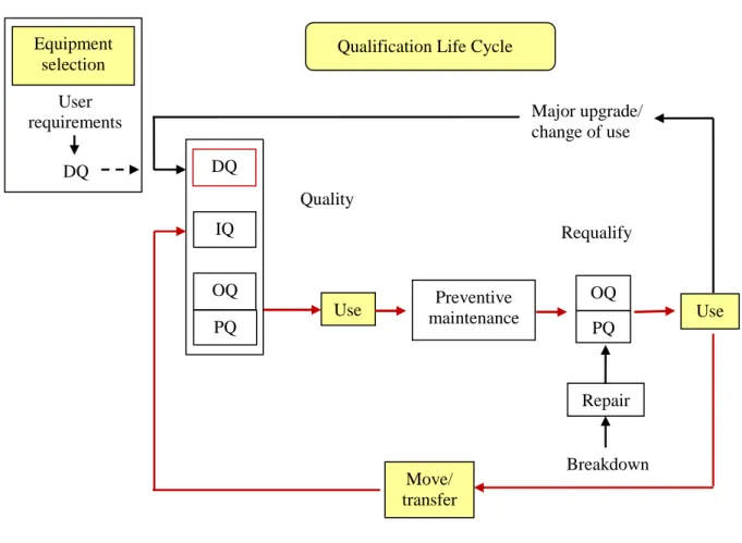
Equipment qualification is one of the first steps in analytical method validation and it is a formal systematic process that provides confidence and documented evidence that an instrument is fit for its intended purpose and kept in a state of maintenance and calibration consistent with its use. Qualification is not a single, continuous process but is a result of many discrete activities which have been grouped into four phases: design qualification (DQ), installation qualification (IQ), operational qualification (OQ) and performance qualification (PQ). A typical qualification process is shown in Figure 1.1 (Smith, 2007). Qualification is performed via documented procedures which contains the specific instructions and acceptance criteria that need to be executed and met (Bedson and Rudd, 1999).
Design qualification covers all the procedures prior to the installation of the system in the selected environment. This is the `planning part´ of the EQ process where user requirements specifications and the details for purchasing the equipment are defined (Bedson and Rudd, 1999). Typically DQ includes: (a) description of the intended use of the equipment; (b) selection of the analysis technique, of the technical, environmental and safety precautions, final selection of the supplier and of the
8
equipment; and (c) development and documentation of final functional and operational specifications (Papadoyannis and Samanidou, 2005).
Figure 1.1. A typical qualification lifecycle (Smith, 2007).
Installation qualification is a process used to establish that the instrument was received as specified and installed correctly according to the design requirements in an environment suitable for its operation. Proper installation ensures proper functioning of the equipment.
Operational qualification verifies the key aspects of instrumental performance in the absence of any contributory effects which may be introduced by the method. This involves checking the performance of individual instrument modules to provide evidence that they are operating correctly and within specification. Operational qualification should be carried out after the initial installation of the equipment and must be repeated at regular stages during the life of the instrument depending on the
Equipment selection
User requirements
DQ
Qualification Life Cycle
Major upgrade/ change of use Requalify Move/ transfer Breakdown Quality DQ IQ OQ PQ
Use maintenance Preventive
OQ PQ
Use
9
manufacturer´s recommended intervals, the required performance of the instrument, the nature and usage of the instrument, the environmental conditions where the instrument is installed and the time that the instrument performance is operating under control. In some instances, event-driven OQ is repeated whenever there is (a) routine maintenance, servicing and replacement of parts, (b) movement or relocation, (c) interruption to services and/or utilities, (d) modification or upgrades, (e) troubleshooting/faultfinding after PQ failure.
Performance qualification (PQ) documents the performance of the instrument on continuous operation. It can be considered as having two stages: (1) an initial PQ which is performed after OQ in order to verify the overall performance of the system via a holistic test which involves analyzing a test mixture on a test column; and (2) an ongoing PQ (system suitability checking) to provide continued evidence of the suitability of the instrument´s performance (Bedson and Rudd, 1999). In the event that PQ fails to meet the specifications, the instrument requires maintenance or repair or calibration and the relevant PQ test(s) should be repeated to ensure that the instrument remains qualified. In all these undertakings, standard operating procedures must be maintained and all the activities are recorded (Bansal, et.al., 2004).
1.2.1.1. Instrument maintenance, calibration and verification
Laboratory instrument has to be maintained on a regular basis in order to avoid system failure during operation. Its performance must be reviewed on a regular basis in order to ensure that the instrument is reliable and continues to comply with the requirements specified by the user. Proper maintenance not only makes sense from a scientific point of view but also for financial reasons. Any routine maintenance procedure suggested by the vendor should be followed. The laboratory can also establish its own set of maintenance procedures based upon how the instrument is being used, the types of samples run, and the number of users (considering their level of training and expertise) that have access to the instrument.
Section 5.5.2 of the ISO 17025 standard (2005) states that “…Calibration programmes shall be established for key quantities or values of the instruments where
10
these properties have a significant effect on the results. Before being placed into service, equipment (including that used for sampling) shall be calibrated or checked to establish that it meets the laboratory´s specifications requirements and complies with relevant standard specifications. It shall be checked and/or calibrated before use.” Hence, for laboratories adopting a quality system it is necessary that instrument calibration and verification are put into practice.
Calibration and verification are two terms that are often used incorrectly but each has distinct meaning. ISO/IEC Guide 99 (2007) defines calibration as the “operation that, under specified conditions, in a first step, establishes a relation between the quantity values with measurement uncertainties provided by measurement standards and corresponding indications with associated measurement uncertainties and, in second step, uses this information to establish a relation for obtaining a measurement result from an indication.” Calibration is also used to describe the process where several measurements are necessary to establish the relationship between response and concentration which results to the generation of a calibration graph (Prichard and Barwick, 2007).
Verification, on the other hand, is defined by ISO/IEC Guide 99 (2007) as the “provision of evidence that a given item fulfills specified requirements” -Performance verification of an analytical instrument involves comparison of the test results with specifications. It includes testing and requires the availability of clear specifications and acceptance criteria. Calibration permits the estimation of errors of the measuring instrument or the assignment of values to marks on arbitrary scales, whereas, verification of an instrument provides a means of checking whether the deviations between the values indicated by the instrument and the known values of a measured quantity are acceptable or not (Prichard and Barwick, 2007).
The instrument performance will continue to deteriorate through time due to wear and ageing of the components. While routine maintenance can counteract this reduced performance in a short term, it will be inevitable in the long run. However, it is necessary to establish that the instrument continuously meets the minimum established criteria or acceptance limits. These acceptance criteria should not exceed more than what is appropriate for the actual needs of the laboratory otherwise if the established
11
acceptance criteria are unnecessarily high then it will be difficult to maintain the instrument “within specification”. In common applications, when confronted with having more than one instrument of the same type but are from different manufacturers and having different ages, the performance testing process is simplified by choosing less stringent common acceptance criteria that all of the instruments can meet (Currell, 2000).
1.2.1.2. LC-MS performance verification
For an LC-MS system, it is necessary to verify the performance of LC and the MS separately. Likewise, it is important that the coupling of these two instruments demonstrates satisfactory performance. The complexity of the instrumentation often dictates the level of verification necessary to be performed. This is the case with hyphenated instruments such as the LC-MS especially when the individual systems come from different vendors. Normally, the performances of the individual systems (the LC and the MS) are readily verified according to each of the vendor´s procedure. However, when dealt with a coupled system such as LC-MS, the verification of its performance as a whole system can be a quite complicated process. The laboratory is responsible for ensuring that the performance of the LC-MS is still under quality control. To achieve this purpose, the laboratory can choose to develop its own verification process that is scientifically sound, straightforward to use and adequate for the intended application. In this context, it is proposed to use a method with known performance characteristics in order to verify the whole LC-MS system.
1.2.1.2.1. HPLC performance verification
The performance of an HPLC system can be evaluated by examining the key attributes of the various modules comprising the system, followed by a holistic test that takes into account performance of the integrated system as a whole. According to Lam (2004), these are the key performance attributes of the HPLC modules that are checked: a) Pump module – flow rate accuracy, gradient accuracy and precision,
pressure test
12
c) UV-Visible detector module – wavelength accuracy, linearity of response, noise and drift
d) Column heating module – temperature accuracy and temperature stability After a verification test, the results are assessed in terms of the predefined acceptance criteria. These criteria had been defined from previously set user requirements. Whenever failure is indicated after the performance verification tests, an impact assessment should be made to evaluate the effect of the failure on the quality of the data generated by the system.
1.2.1.2.2. Column performance verification
The chromatographic column influences the effective separation of the analytes in a given sample. Before a column is purchased, it is necessary to obtain some information regarding column specifications and performance characteristics which are valuable for method development and routine use. The quality or performance of the column deteriorates through time depending on how the operator uses it. Eventually, an HPLC column will decrease its efficiency hence it is important to monitor its performance. The following parameters are normally determined in a given test compound: (a) number of plates (N), (b) peak tailing factor (or symmetry factor) and (c) capacity factor (k´).
The plate number (N) measures the ability of a column to produce a peak that is narrow in relation to its retention time. It is generally estimated from a peak (a neutral compound) which appears towards the end of the chromatogram in order to get a reference value. It is dependent on the chosen solute and the operational conditions adopted.
Symmetrical peaks are always preferred since peaks with poor symmetry can result to inaccurate measurements of plate number and resolution, imprecise quantitation, poor resolution leading to undetected minor bands in the peak tail a poor reproducibility of retention times (Snyder, et.al., 1997). The quality of the peak shape is measured in terms of the tailing factor (Tf).
13
The capacity factor or retention factor (k´) is a measure of the time the sample component resides in the stationary phase relative to the time it resides in the mobile phase; it expresses how much longer a sample component is retarded by the stationary phase than it would take to travel through the column with the velocity of the mobile phase (IUPAC, 1993).
1.2.1.2.3. Mass spectrometer performance verification
The satisfactory performance of the mass spectrometer depends on its calibration and proper functioning of the instrument system such as electronics and vacuum systems, among others. Normally, an MS instrument has built-in options for checking the overall condition of the instrumental system.
The mass spectrometer provides accurate measurement only if the m/z axis is properly calibrated. The calibration is performed using automated procedures often included in the instrument software. During the calibration procedure, a mixture of a MS calibrants (well-characterized reference compounds) are introduced in the ion source of the mass spectrometer, ionized and monitored their spectrum. The calibration of the m/z axis can be performed by comparing the theoretical and the experimental spectrum of the reference compound.
A calibration standard mass must have the following characteristics: (a) it should yield a sufficient number of regularly spaced abundant ions across the entire mass scan range; and (b) it should be chemically inert (Dass, 2007). There are several compounds that were proposed to be used as calibration standards in electrospray LC-MS. The proposed calibrants include (a) cesium iodide or cesium carbonate cluster ions, (b) poly(ethylene glycol) (PEG) and poly(propropylene glycol) (PPG), (c) proteins such as the peptide MRFA and myoglobin, (d) Ultramark 1621, a mixture of fluorinated phosphazenes, (e) water cluster ions and (f) sodium trifluoroacetate cluster ions (Niessen, 2006).
14
1.2.1.2.4. System Suitability Test
The system suitability test for a method is based on the concept that the equipment, electronics, analytical operations and samples to be analyzed constitute an integral system that can be evaluated as such (ICH, 2005). The parameters necessary to be established for system suitability test will depend on the particular method being tested. The parameters and the criteria must be carefully chosen so as to provide unbiased results. System suitability tests are usually done at the start of the analysis but depending on the length of the run or the importance of the sample results, system suitability test may also be performed during and following the analysis (Wells and Dantus, 2005).
1.2.1.2.5. Analytical method performance characteristic determination
A newly developed analytical method must at least provide some analytical figures of merit or performance characteristics for future reference to other analysts that will adopt the method in the future (Krull and Swartz, 1999).
The typical method characteristics that need to be evaluated are: selectivity/specificity, accuracy, precision (repeatability, intermediate precision), limit of detection (LOD) or detection limit, limit of quantification (LOQ) or quantification limit, and linearity and linear range. These definitions are in accordance with the ICH Harmonized Tripartite Guideline for the Validation of Analytical Procedures (2005):
a) Specificity – the ability of to assess unequivocally the analyte in the presence of other components which may be expected to be present.
b) Accuracy – expresses the closeness of agreement between the value which is accepted either as a conventional true value or an accepted reference value and the value found.
c) Precision – expresses the closeness of agreement (degree of scatter) between a series of measurements obtained from multiple sampling of the same homogeneous sample under the prescribed conditions. Precision may be considered at three levels: repeatability, intermediate precision and reproducibility.
15
d) Limit of detection – the lowest amount of analyte in a sample which can be detected but not necessarily quantitated as an exact value.
e) Limit of quantification – the lowest amount of analyte in a sample which can be quantitatively determined with suitable precision and accuracy.
f) Linearity – the ability (within a given range) to obtain test results which are directly proportional to the concentration (amount) of analyte in the sample. g) Linear range – the interval between the upper and lower concentration
(amounts) of analyte in the sample (including these concentrations) for which it has been demonstrated that the analytical procedure has a suitable level of precision, accuracy and linearity.
The method´s performance characteristics should be based on the intended use of the method and the requirements may need to be assessed depending upon the nature of the method and test specifications.
1.3. Documentation in laboratory practice
Documentation is a critical part of a quality assurance system. Laboratories should maintain and control documents related to sampling procedures, calibration procedures, analytical and test methods, data collection and reporting procedures, auditing procedures and checklists, sample handling and storage procedures, computation and data validation procedures, quality assurance manuals, quality plans, sampling data sheets and specifications (Ratliff, 2003).
Standards and regulations require that the laboratory should have written, clear and detailed procedures for all the activities that are performed in the laboratory. A standard operating procedure (SOP) describes the set of instructions a technician or an analyst follows when carrying out an analysis or a process (Kenkel, 2000). SOP forms part of the hierarchy of quality documentation. Several advantages can be cited for having a readily accessible, user-friendly, agreed set of SOPs: they provide evidence that all procedures are in place; they reflect the laboratory´s commitment to quality
16
standards; they ensure standardization of procedures; they reduce variability and errors; they provide an invaluable platform for staff training and support (Carson and Dent, 2007).
17
2. EXPERIMENTAL
These were the standards, the reagents and the instrumentation used for carrying out the different verification processes.
2. 1. Chemicals and Instrumentation
2.1.1. Standards and Reagents
HPLC performance verification Caffeine, Merck
Column verification
Uracil, 98%, Merck
Acetophenone, 99%, Sigma, USA Toluene, GC grade, Merck
LCQ MS calibration Caffeine, Sigma
MRFA (L-methionyl-arginyl-phenylalanyl-alanine acetate·H2O),
Sigma
Ultramark 1621, Sigma HPLC-MS analysis
1-naphthylacetamide PESTANAL®
, 99%, Sigma-Aldrich 1-naphthoxyacetic acid, 98%, Aldrich
2-naphthoxyacetic acid PESTANAL®
, 98%, Sigma-Aldrich HPLC performance verification
Water , LC-MS grade, Fluka Sigma Aldrich Methanol, LC-MS grade, Fluka Sigma Aldrich Acetonitrile, LC-MS grade, Fluka Sigma Aldrich Acetone, GC grade, Merck
Column verification
Water, LC-MS grade, Fluka Sigma Aldrich Acetonitrile, LC-MS grade, Fluka Sigma Aldrich LCQ MS calibration
18
Methanol, LC-MS grade, Fluka Sigma Aldrich Acetonitrile, LC-MS grade, Fluka Sigma Aldrich HPLC-MS analysis
Methanol, LC-MS grade, Fluka Sigma Aldrich Water, LC-MS grade, Fluka Sigma Aldrich for mobile phase preparation
Glacial acetic acid, analytical grade, Merck
2.1.2. Instrumentation
2.1.2.1. Liquid chromatography
Dionex HPLC system (Dionex Softron GmbH, Germany) which consists of
- SOR-100A-6 solvent rack
- P680 A DGP-6 high-precision gradient pump with 3 solvent channels each for the left and right pump
- ASI-100 automated sample injector
- TCC-100 thermostatted column compartment - UVD 170U UV-Vis diode array detector
- Chromeleon 6.70 chromatography management software
Accela HPLC system (Thermo Electron San Jose, USA) which consists of
- quarternary pump with vacuum degasser
- autosampler which also includes the column oven tray compartment heater/cooler
- PDA detector
- Xcalibur data system
Ascentis®
Express RP-Amide, 10cm x 2.1 mm, 2.7 μm (Supelco)
LiChrospher 100 RP-18 (5µm) HPLC cartridge, 125mm x 4mm (Agilent)
19
2.1.2.2. Mass spectrometry
Finnigan LCQ quadrupole ion trap mass spectrometer (Thermo Electron San Jose, USA):
electrospray (ESI) and atmospheric pressure chemical ionization (APCI) sources
ion trap mass analyzer Xcalibur® data system 2.1.2.3. Other instruments
Analytical balance (Mettler Toledo AT261 Delta Range)
Calibrated digital thermometer with thermal probe (Testo 945), calibrated at 0 to 200°C by ENAC
2.2. Experimental Procedure
This section describes the different activities that were performed in order to accomplish the objectives of the study. The different procedures for the performance verification of the HPLC, the column, the mass spectrometer and the LC-MS are presented.
2.2.1. HPLC performance verification
The detailed procedure for the performance verification of the Dionex HPLC-UV-Vis is described in the document Instructions for the Performance Verification of the
Dionex HPLC System with UV/Vis Diode Array Detector (SOP/CECEM/EQP/02/01).
The verification included the determination of the performance attributes of the different HPLC modules: pump, autosampler, column oven and detector.
The verification of the Dionex HPLC-UV was performed using a LiChrospher 100 RP-18 column, 125mm x 4mm, 5µm (Agilent) instead of a restriction capillary. The column oven temperature was set to 25°C, except in column oven verification. The column and the system were allowed to equilibrate for at least 15 minutes before
20
starting with data acquisition unless otherwise specified. After the test, the results were compared with the set acceptance criteria.
2.2.1.1. Preparation of caffeine solutions
A stock solution of caffeine with a concentration of 1000 mg L-1 was prepared
by weighing 10 mg of caffeine standard and dissolving it in 10 mL of water. This stock solution was used in the preparation of different concentrations (300, 220, 140, 75, 60,
40, 10 and 5 µg mL-1) of caffeine standard in water. All the resulting solutions were
weighed and their masses were recorded.
2.2.1.2. Performance verification of the pump
The performance verification of the pump of the HPLC was done through the determination of flow rate accuracy, flow rate precision, and gradient accuracy.
2.2.1.2.1. Determination of flow rate accuracy
The flow rate accuracy was determined by measuring the time elapsed to fill a 10 mL flask with water flowing from a solvent channel at a rate of 1 mL/min. The flow rate was calculated using the formula below:
(min) fill to time (mL) flask of volume min mL rate flow
The measurement was done in triplicate and then the average flow rate was compared with the set flow rate.
2.2.1.2.2. Determination of flow rate precision
The mobile phase (85:15 (v/v) water:acetonitrile) was set at a flow rate of 1 mL/min. The acquisition time was 6 minutes and the response of the UV detector was monitored at 272 nm. The flow rate precision was determined by repeated injections (10
times) of 5 µL of a 140 µg mL-1 caffeine standard solution. The retention time of
caffeine was obtained after each injection. The %RSD of the retention time was used to evaluate the flow rate precision.
21
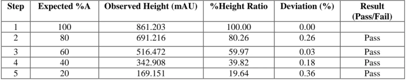
2.2.1.2.3. Determination of gradient accuracy
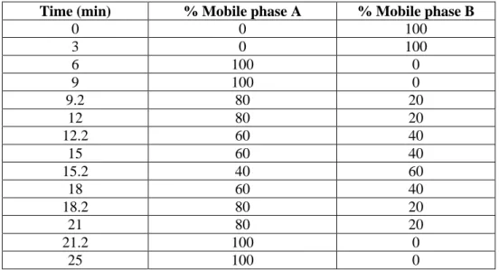
This determination was necessary to be performed for all the channels of the pump, using two channels for each determination. One channel was filled with mobile phase A (99.5:0.5 (v/v) methanol:acetone) while another channel was filled with mobile phase B (methanol). The flow rate was set to 1 mL/min and UV detection at 265 nm. The program for gradient accuracy testing is shown in Table 2.1. By performing a blank run, a chromatogram was obtained showing the absorbance change (expressed as height) as gradient changes from 100%B to 100%A and then back to 100%B. The gradient accuracy was calculated from the relative heights (expressed as %Height ratio) of %A (in each step gradient) to 100%A. The calculated %Height ratio was compared with the set value for %A.
Table 2.1. Program for gradient accuracy testing.
Time (min) % Mobile phase A % Mobile phase B
0 0 100 3 0 100 6 100 0 9 100 0 9.2 80 20 12 80 20 12.2 60 40 15 60 40 15.2 40 60 18 60 40 18.2 80 20 21 80 20 21.2 100 0 25 100 0
2.2.1.3. Performance verification of the autosampler
The performance of the autosampler was verified by determination of injection volume precision, injection volume linearity and carryover.
Equation 2.2 100%A of Height %A of Height ratio %Height
22
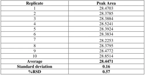
2.2.1.3.1. Determination of injection volume precision
The mobile phase (85:15 (v/v) water:acetonitrile) was set at a flow rate of 1 mL/min. The acquisition time was 6 minutes and the response of the UV detector was monitored at 272 nm. The injection volume precision was determined by repeated
injections (10 times) of 5 µL of a 140 µg mL-1 caffeine standard. The peak area of
caffeine was obtained after each injection. The %RSD of peak area was used to evaluate the flow rate precision.
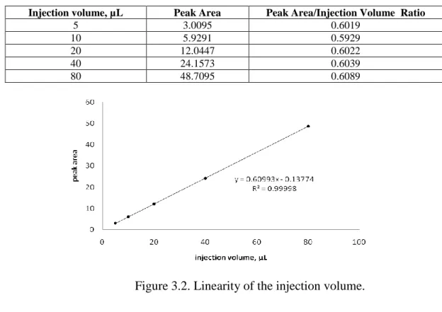
2.2.1.3.2. Determination of injection volume linearity
The mobile phase (85:15 (v/v) water:acetonitrile) was set at a flow rate of 1 mL/min. The acquisition time was 6 minutes and the response of the UV detector was monitored at 272 nm. The injection volume linearity was determined by injecting 5, 10,
20, 40 and 80 μL of a 10 µg mL-1 caffeine standard. The peak area of caffeine was
obtained after each injection. A linearity plot (peak area vs. injection volume) was constructed and the linear regression coefficient (r) was obtained. The ratio between the peak area and the volume injected was calculated and the %RSD of the peak area/injection volume was also determined.
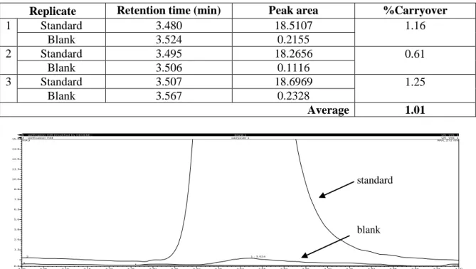
2.2.1.3.3. Determination of carryover
The mobile phase (85:15 (v/v) water:acetonitrile) was set at a flow rate of 1 mL/min. The acquisition time was 6 minutes and the response of the UV detector was
monitored at 272 nm. The carryover was determined by injecting 5 μL of a 75 µg mL-1
caffeine standard. Immediately after running the standard, a 5 μL mobile phase was
injected. The measurement was done in triplicate. The peak area of caffeine was determined in the standard and blank injections. The %carryover was calculated as follows: Equation 2.3 x100 standard in caffeine of area peak blank in caffeine of area peak %Carryover
23
2.2.1.4. Performance verification of the column oven
The column oven performance verification was done by determining the column oven accuracy, column oven temperature precision and column oven temperature stability. Instead of the column, an LC zero dead volume union was used to connect the column inlet and outlet tubings. The flow rate for water was set at 0.1 mL/min. A calibrated digital thermal probe (Testo 945) was used to measure the temperature inside the column oven. The measured temperatures were corrected using the correction factors cited in the thermometer´s calibration certificate.
2.2.1.4.1. Determination of column oven temperature accuracy
The column temperature was set to 20ºC. After the set temperature was reached, the temperature was recorded every three minutes. Three temperature readings were obtained. The difference between the corrected temperature and the set temperature was
calculated. The same procedure was done at the set temperatures of 40ºC and 60ºC.
2.2.1.4.2. Determination of column oven temperature precision
The column temperature was set to 40ºC. After the set temperature was reached, the temperature was recorded. The temperature was decreased by setting to 35 ºC. The temperature was then again set to 40ºC and the temperature was recorded after the set temperature was reached. This procedure was done once more to obtain triplicate readings. The maximum difference between the 3 temperature readings was calculated. 2.2.1.4.3. Determination of column oven temperature stability
The column temperature was set to 40ºC. After the set temperature was reached, temperature measurement was started. Temperature readings were obtained every 4 minutes and for a period of 1 hour. A temperature stability plot was made between the temperature readings and time.
2.2.1.5. Performance verification of the detector
The performance verification of the detector was conducted by determining the linearity of detector response and the noise and drift.
24
2.2.1.5.1. Determination of the linearity of detector response
The mobile phase (85:15 (v/v) water:acetonitrile) was set at a flow rate of 1 mL/min. The acquisition time was 6 minutes and the response of the UV detector was monitored at 272 nm. The linearity of detector response was determined by injecting 5
μL each of 10, 60, 140, 220 and 300 µg mL-1
caffeine standards. The peak area of caffeine was obtained after each injection. A linearity plot (peak area vs. injection concentration) was constructed and the linear regression coefficient was obtained. The ratio between the peak area and the concentration was calculated and the %RSD of the peak area/concentration was also determined.
2.2.1.5.2. Determination of noise and drift
This determination was necessary to be performed for all the channels of the pump, using two channels for each determination. To determine the noise and drift, one channel was filled with water and the other channel was filled with methanol. The flow rate of the mobile phase (50:50 (v/v) methanol:water) was set to 1 mL/min. The UV detector was turned on and the system was stabilized for at least one hour before starting the data acquisition. The acquisition time was 20 min., and the response of the UV detector was monitored at 254 nm. A blank injection was performed in order to obtain the baseline plot. The baseline plot was divided into 20 segments and the noise and drift was calculated in each segment. The noise and drift was calculated using the Chromeleon software. The noise corresponds to the distance between two parallel lines through the measured minimum and maximum values and the regression line. The drift was estimated as the slope of the regression line.
2.2.2. Column Performance verification
The performance of the Ascentis® Express RP-Amide column (10cm x 2.1 mm,
2.7 μm, Supelco) was evaluated using two HPLC instruments: Accela HPLC-UV and
Dionex-HPLC UV/Vis. The procedure of the test is described in the document entitled
Instructions For Verification Of Column Performance (Ascentis Express® RP-amide, 10 cm x 2.1 mm x 2.7 µm, Supelco) (SOP/CECEM/EQP/07/01).
25
2.2.2.1. Preparation of test solution
The stock solutions of uracil (1mg mL-1), acetophenone (1mg mL-1) and toluene
(10 mg mL-1) were prepared as follows: weighing 5 mg of uracil and dissolving in 5 mL
of 50:50 (v/v) acetonitrile:water solution; taking 5µL of acetophenone and mixing with 5 mL of 50:50 (v:v) acetonitrile:water solution; taking 58 µL of toluene and mix with 5 mL of 50:50 (v:v) acetonitrile:water solution. The test solution was prepared by taking
aliquots of 20 µL of 1 mg mL-1uracil, 30 µL of 1mg mL-1of acetophenone, 240 µL of 10
mg mL-1 toluene and mixing with 710 µL of 50:50 (v:v) acetonitrile:water in a glass
vial.
2.2.2.2. HPLC run
These were the chromatographic conditions used: mobile phase: 50:50 acetonitrile:water; flow rate: 0.5 mL/min; injection volume: 1 µL; acquisition time: 4 min; temperature: 25°C; UV detection: 254 nm.
The HPLC column was installed in the HPLC instrument and was allowed to equilibrate with the mobile phase for at least 15 minutes. The test compound was injected and after the chromatographic run the retention times of the eluted peaks were compared with the retention times indicated in the test chromatogram from the vendor.
The number of plates (N), tailing factor (Tf) and capacity factor (k´) for the last peak
(toluene) were calculated using Equations 2.4, 2.5 and 2.6, respectively. The calculated values were compared with the vendor´s specifications.
N was calculated from the following equation:
where tR stands for the retention time and w0.5 for the peak width at half height
The tailing factor (Tf) was calculated as:
where W0.05 is the peak width at 5% height and f is the front half-width at 5% of the
peak height. 2 h R w t 5.545 N Equation 2.4 2f W T 0.05 f Equation 2.5
26
The capacity factor or retention factor (k´) was calculated as
where tR stands for the retention time and t0 for the retention time of the unretained
compound or dead time.
2.2.3. Mass spectrometer performance verification
The procedure for this determination can be found on the document Instructions
for Performance Verification of the LCQ MS (Finnigan) SOP/CECEM/EQP/05/01. The
ion gauge pressure and the convectron gauge pressure were always checked before starting any MS analysis to ensure that the vacuum system is working properly. To demonstrate that the instrument´s major electronic systems were operating satisfactorily, the built-in option “Diagnostic Test” of the software was selected. With this test, the power supplies, API temperatures, lenses and RF were tested. The instrument displays a Pass/Fail result to indicate whether all parts are working properly or not.
2.2.3.1. Mass spectrometer calibration
The mass spectrometer was calibrated by following the procedure described in the document that already exists in the laboratory entitled Instrucciones para la Calibracion
y Tuning del Espectrómetro de Masas LCQ (Finnigan) (PNT 035100 APR/103).
2.2.3.1.1. Preparation of the calibration solution
The calibration solution was prepared from the stock solutions of caffeine (1mg
mL-1), MRFA (5 nmol/μL) and Ultramark 1621 (0.1%). The caffeine stock solution was
prepared by weighing 1 mg caffeine and dissolving it in 1 mL methanol; the MRFA stock solution by weighing 3.0 mg of L-methionyl-arginyl-phenylalanyl-alanine
acetate·H2O (MRFA) and dissolving in 1 mL of 50:50 (v/) methanol:water solution; and
Ultramark 1621 solution by dissolving 10µL of Ultramark 1621 in 10 mL of acetonitrile. A 5 mL calibration solution was prepared by pipetting the following into a clean, dry vial: 100 µL caffeine stock solution, 5 µL MRFA stock solution, 2.5 mL
Equation 2.6 0 0 R ´ t t t k
27
Ultramark 1621 stock solution, 50 µL glacial acetic acid, and 2.34 mL 50:50 (v/v) methanol: water solution.
2.2.3.1.2. Instrument Setup
The fused silica capillary used for calibration was connected in the ESI probe before the probe assembly was installed in the detector. The ESI probe was configured to work at low flow rate infusion. The syringe was filled with the calibration solution and was connected directly to the grounded fitting of the probe assembly.
2.2.3.1.2. Calibration
The instrument was set to the ESI positive mode and the calibration solution was infused at a flow rate of 3μL/min. The ESI source parameters were set to the following values: Sheath gas flow rate: 40; Aux. Gas flow rate: 0; Spray voltage: 4.00; Capillary temperature: 275; Capillary voltage: 3.00; Tube lens offset: 30.00. The Define scan
parameters used were: Scan mode: MS; Scan type: Full; MSn power: 1; Number of
Microscans: 2; Maximum inject time: 200; Input Method: From Mass 150 to 2000; Source Fragmentation: Off.
The ESI operation was first tested by observing the singly-charged positive ions for caffeine, MRFA, and Ultramark 1621. Before calibration was done, the instrument response was optimized by automatic tuning (via the instrument´s Tune program) using the caffeine peak of m/z 195. Afterwards, the automatic calibration was begun by selecting the instrument´s Calibrate option. Once the calibration has finished, a calibration report was displayed showing the success/fail result of the calibration. After calibration, the fused silica capillary was removed from the ESI probe and was replaced with a new capillary. The detector was flushed with acetonitrile for cleaning.
2.2.4. LC-MS performance verification
The proper functioning of the LC-MS was verified by using a method that was developed in the CECEM laboratory. The method involves the LC-MS/MS analysis of
1-28
naphthylacetamide). For the purpose of this investigation, it was only necessary to determine the possible conditions in which this method can be adopted in the Finnigan LCQ MS and determine some quality parameters such as limit of detection, limit of quantification, linearity and precision, which can serve as a reference for verifying the performance of the whole LC-MS system in the future. The procedure for the LC-MS verification can be found in the document entitled Performance Verification of an
LC-MS System (SOP/CECEM/EQP/08/01) found in the Appendix.
2.2.4.1. Tuning with the analytes
Before starting with any LC-MS determination, the response on the MS detector
has to be optimized by tuning the tube lens with 1-naphthylacetamide (5 µg mL-1) and
1-naphthoxyacetic acid (5 µg mL-1) using a 50:50 (v/v) methanol:2mM acetic acid
solution as mobile phase. The standard solution of the analyte was introduced by infusion using the syringe pump. The scan parameters used were as follows: Scan mode:
MS; Scan type: Full; MSn power: 1; Number of Microscans: 3; Maximum inject time:
100; Input Method: From Mass 50 to 300; Source Fragmentation: Off. The tuning process was done by using the Tune program of the instrument software. Semi-automatic tune was done for the other MS parameters (capillary voltage and tube lens offset voltage).
2.2.4.2. Establishment of the chromatographic and MS detection conditions 2.2.4.2.1. Liquid chromatographic conditions
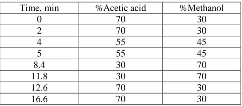
From the original method, the same gradient elution program was employed but the flow rate was decreased to 300 μL/min due to the limitations imposed by the HPLC-MS instrument. The mobile phase A (2mM acetic acid) was prepared by adding 115 μL of glacial acetic acid to 1L of water. Mobile phase B is methanol and hence preparation was not necessary. The mobile phase composition is shown in Table 2.2. Finally, these were the conditions that were established to be adequate in performing the analysis:
Column: Ascentis Express RP-Amide, 10 cm x 2.1 mm, 2.7µm Mobile Phase: 2 mM acetic Acid: Methanol
Flow rate: 0.300 mL/min Column Temperature: 50°C Injection volume: 5 µL
29
Table 2.2. Gradient elution program.
Time, min %Acetic acid %Methanol
0 70 30 2 70 30 4 55 45 5 55 45 8.4 30 70 11.8 30 70 12.6 70 30 16.6 70 30 2.2.4.2.2. MS conditions
The MS/MS detection settings were established in terms of the ESI source parameters, isolation width, normalized collision energy, activation Q and activation time. The optimum parameters were chosen such that the mass chromatogram shows the maximum product ion intensities for a selected precursor ion. Table 2.3 summarizes the optimal values of the MS parameters for this determination.
Table 2.3. MS detection parameters.
Parameters 1-Naphthylacetamide 1-Naphthoxyacetic acid
2-Naphthoxyacetic acid ESI mode positive negative negative ESI Source parameters
Sheath gas (arb) 70 53 53 Auxiliary gas (arb) 40 48 48 Spray voltage (kV) 4 4 4 Capillary Temperature (°C) 250 250 250 Capillary voltage (V) 9 -17 -17 Tube lens offset (V) -15 15 15 Precursor (m/z) 186.1 201.1 201.1 Product ion for quantitation (m/z) 141 143 143 Product ion for confirmation (m/z) 169 157 157 Isolation width (m/z) 1.5 1.5 1.5 Normalized collision energy
(%NCE)
25 29 28.5
Activation Q 0.40 0.40 0.40 Activation time (msec) 0.30 0.30 0.30
30
2.2.4.3. Determination of quality parameters
The following quality parameters were evaluated for the determination of 1-naphthylacetamide, 1-naphthoxyacetic acid and 2-naphthoxyacetic acid by HPLC-MS/MS: limit of detection, limit of quantitation, linearity and precision (repeatability).
These analytes were detected using the Finnigan LCQ MS analyzer equipped with an
electrospray ion source operated in the positive mode (for 1-NAD detection) and negative mode (for 1-NOA and 2-NOA detection).
2.2.4.3.1. Preparation of standard solutions
A 1,000 µg mL-1 stock solution of each of the analytes was prepared from the
following solid standards: 1-naphthoxyacetic acid, 98% purity; 2-naphthoxyacetic acid, 98% purity; 1-naphthylacetamide, 99% purity. A 5.00 mg solid standard was weighed and dissolved in 5 mL of methanol.
An intermediate standard (10 µg mL-1) was made by pipetting 30 µL of 1,000 µg
mL-1 1-NOA, 30 µL of 1,000 µg mL-1 2-NOA and 30 µL of 1,000 µg mL-1 1-NAD and
mixing with 3.910 mL of methanol. From this 10 ppm intermediate standard, working
calibration standard solutions between 0.1 and 1 µg mL-1 was used for linearity,
precision and recovery determinations. Another intermediate standard of 0.200 µg mL-1
concentration was prepared from 10 µg mL-1 standard. The 0.200 µg mL-1 standard was
used for the preparation of standards (2.5 ng mL-1 to 50 ng mL-1) used in LOD
determination. The mass of the aliquot taken and mass of the final solution were recorded and used for the calculation of the final concentration.
2.2.4.3.2. Identification of the analytes
The analytes were identified by injecting individual standard solutions of each
analyte at 0.5 µg mL-1. From the resulting chromatogram, the retention times were
noted and the mass tandem spectrum was examined for confirming the presence of the precursor and product ions.
31
2.2.4.3.3. Determination of limit of detection (LOD) and limit of quantitation (LOQ) The instrument LOD was determined by preparing dilute standard solutions
from a 0.200 µg mL-1 standard containing a mixture of 1-naphthoxyacetic acid,
2-naphthoxyacetic acid and 1-naphthylacetamide. The LOD and LOQ were estimated based on the signal-to-noise ratio (S/N) measurement. The dilute standard solutions were subjected into the LC-MS run, and the chromatogram obtained was inspected for
the S/N ratio. LOD was estimated as the standard concentration (ng mL-1) which gave a
S/N ratio around 3. Finally, the LOD was expressed as the amount (ng) of analyte injected by the expression:
LOD (ng) = Concentration (ng/µL) * volume (µL) injected
The LOQ was estimated from the LOD data. LOQ (S/N ≈ 10) was derived from the expression:
LOQ = LOD * 3.3
2.2.4.3.4. Determination of linearity
The linearity was determined by preparing standard solutions containing the
three analytes from a concentration similar to the LOQ until around 1 µg mL-1. The
standards were injected starting from the lowest to the highest concentration. At the end, the peak areas were determined by manual integration on the Xcalibur software. A plot of peak area vs. concentration was made and the linear regression parameters were obtained. The linearity was evaluated in terms of the regression coefficient (r).
2.2.4.3.5. Determination of precision (repeatability) and relative error
The instrument precision was determined by performing 6 injections of a standard solution containing the analyte at a middle concentration level. The retention times and peak areas (manually integrated) were obtained from each run. The injection precision was evaluated in terms of the %RSD of the retention time and peak area. The precision was also evaluated in terms of the %RSD of the calculated concentration when the standard is quantified as unknown sample using the linear calibration curve.
Equation 2.8 Equation 2.7
32
Moreover, the error associated on the quantification was estimated by the %Relative error, which was calculated as follows:
Equation 2.9 100 x ion concentrat l theoretica ion) concentrat cal theoreti curve n calibratio the from obtained tion (concentra error %Relative
33
3. RESULTS AND DISCUSSION
Quality control is an important aspect of an analytical laboratory. Quality control measures must be designed and followed because they provide a mechanism in achieving reliable data. For a typical LC-MS determination, these are some of the measures necessary for obtaining quality results: (1) performance verification of HPLC, (2) performance verification of column, (3) performance verification of the MS system, (4) performance verification of the LC-MS system, and (d) documentation of the procedures necessary for carrying out these tasks.
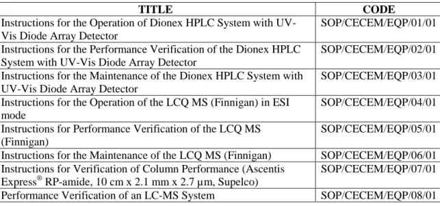
After carrying out the different activities mentioned above, the corresponding documents were generated. The list of documents with the codification is shown in Table 3.1. All of the documents can be found in the Appendix section.
Table 3.1. Summary of the generated documents.
TITLE CODE
Instructions for the Operation of Dionex HPLC System with UV-Vis Diode Array Detector
SOP/CECEM/EQP/01/01 Instructions for the Performance Verification of the Dionex HPLC
System with UV-Vis Diode Array Detector
SOP/CECEM/EQP/02/01 Instructions for the Maintenance of the Dionex HPLC System with
UV-Vis Diode Array Detector
SOP/CECEM/EQP/03/01 Instructions for the Operation of the LCQ MS (Finnigan) in ESI
mode
SOP/CECEM/EQP/04/01 Instructions for Performance Verification of the LCQ MS
(Finnigan)
SOP/CECEM/EQP/05/01 Instructions for the Maintenance of the LCQ MS (Finnigan) SOP/CECEM/EQP/06/01 Instructions for Verification of Column Performance (Ascentis
Express® RP-amide, 10 cm x 2.1 mm x 2.7 µm, Supelco)
SOP/CECEM/EQP/07/01 Performance Verification of an LC-MS System SOP/CECEM/EQP/08/01
3.1. Performance Verification of the Dionex HPLC-UV
The performance characteristics of the different HPLC modules were verified by determination of the different parameters listed in Table 3.2. In order to carry out these processes and set the acceptance criteria, the operational qualification (OQ) procedures performed by the instrument vendor were consulted along with the proposal from some existing guidelines. Some modifications were made in order to accommodate the current conditions and demands for a given parameter. Caffeine has a well-characterized UV
34
absorption profile and hence was used for most of the verification activities. The column temperature was set to 25°C except during verification of the column oven.
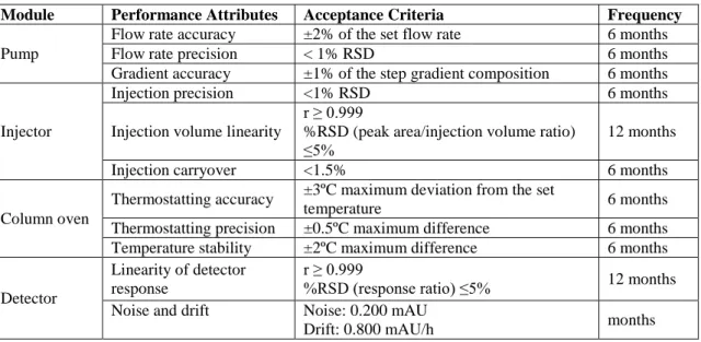
Table 3.2. HPLC performance verification parameters and acceptance criteria.
Module Performance Attributes Acceptance Criteria Frequency
Pump
Flow rate accuracy ±2% of the set flow rate 6 months Flow rate precision < 1% RSD 6 months Gradient accuracy ±1% of the step gradient composition 6 months
Injector
Injection precision <1% RSD 6 months Injection volume linearity
r ≥ 0.999
%RSD (peak area/injection volume ratio) ≤5%
12 months Injection carryover <1.5% 6 months
Column oven
Thermostatting accuracy ±3ºC maximum deviation from the set
temperature 6 months Thermostatting precision ±0.5ºC maximum difference 6 months Temperature stability ±2ºC maximum difference 6 months
Detector
Linearity of detector response
r ≥ 0.999
%RSD (response ratio) ≤5% 12 months Noise and drift Noise: 0.200 mAU
Drift: 0.800 mAU/h months
3.1.1. Verification of the pump
3.1.1.1. Determination of the flow rate accuracy
Pump is an essential component of an HPLC system that ensures an accurate and consistent flow of the mobile phase in order to have an efficient interaction between the stationary phase and the analyte. The flow rate of the mobile phase affects the time the analyte spends in the stationary phase and hence affects the time and degree of separation of the components in a given sample.
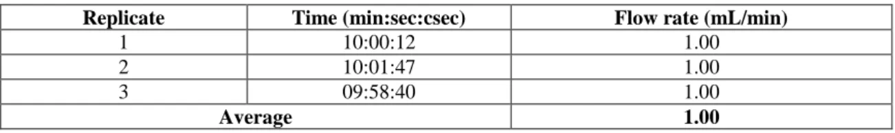
The flow rate accuracy was determined by setting the flow rate of water to 1 mL/min and measuring the time it took to fill a 10-mL volumetric flask. Three replicate analyses were done and the results are shown in Table 3.3. The average flow rate was
1.00 mL/min. Since the acceptance criteria set for the flow rate accuracy was 1.00 ±
35
Table 3. 3. Pump flow rate accuracy results.
Replicate Time (min:sec:csec) Flow rate (mL/min)
1 10:00:12 1.00
2 10:01:47 1.00
3 09:58:40 1.00
Average 1.00
3.1.1.2. Determination of the flow rate precision
The precision of the flow rate was determined by ten injections of 149 µg g-1
caffeine standard. The precision is expressed in terms of the % RSD of the retention times. The results are shown in Table 3.4. The calculated %RSD was 0.25%, so the system passed the set acceptance criteria (<1%RSD).
Table 3.4. Flow rate precision as determined by variability of the retention times of caffeine standard.
Replicate Retention time (min)
1 3.410 2 3.427 3 3.432 4 3.434 5 3.437 6 3.429 7 3.429 8 3.422 9 3.417 10 3.419 Average 3.426 Standard deviation 0.0084 %RSD 0.25
3.1.1.3. Determination of the gradient accuracy
The Dionex HPLC-UV/Vis instrument is designed with left and right pumps, with each pump having three solvent channels. The gradient accuracy test is performed in all the solvent channels. As an example, the result of the gradient accuracy test for the two solvent channels of the left pump is mentioned here.
Gradient accuracy was evaluated by filling the solvent channel C with pure methanol and solvent channel A with 99.5: 0.05 (v/v) acetone:methanol solution. Decreasing the amount of acetone (a UV-active tracer) in the mobile phase leads to a decrease in UV absorption which enabled the accuracy of the gradient mixer to be