Lateral-distortional buckling of continuous steel-concrete composite beam Flambagem lateral com distorção de vigas mistas de aço e concreto contínuas

Lateral-distortional buckling of continuous

steel-concrete composite beam

Flambagem lateral com distorção de vigas mistas

de aço e concreto contínuas

a _{Universidade Federal do Espírito Santo, Departamento de Engenharia Civil, Vitória, ES, Brasil} b _{Universidade Federal de Minas Gerais, Departamento de Estruturas, Belo Horizonte, MG, Brasil}

Received: 09 Aug 2016 • Accepted: 26 Feb 2018 • Available Online:

T. V. AMARAL a

thaisvervloetamaral@gmail.com

J. P. S. OLIVEIRA b

janainapenas@gmail.com

A. F. G. CALENZANI a

afcalenzani@gmail.com

F.B. TEIXEIRA b

felipebarbosateixeira@gmail.com

Abstract

Resumo

In hogging bending moment regions of continuous composite beams the collapse by lateral-distortional buckling (LDB) can occur. The design against LDB according to ABNT NBR 8800:2008 begins with the determination of the elastic critical moment, which depends, among other factors,

of the distribution of the bending moment in the analyzed span, taken into account in the formulation through the modification parameter Cdist. To

assess the analytical formulations prescribed by ABNT NBR 8800:2008, numerical FE models that simulate the LDB behavior of continuous

steel-concrete composite beams were developed in this paper. The different boundary conditions presented in ABNT NBR 8800:2008 were checked using two different models: a simplified model, with a single simply supported span; and models with multiple internal supports and more than one

span. It was observed that the C_dist values prescribed by ABNT NBR 8800:2008 can be unsafe, and therefore new values for C_dist are proposed in this paper.

Keywords: elastic critical moment, lateral-distortional buckling, continuous composite beams.

Nas regiões de momento negativo de vigas mistas contínuas pode ocorrer a flambagem lateral com distorção (FLD). A verificação à FLD pela ABNT NBR 8800:2008 tem como procedimento inicial determinar o momento crítico elástico que depende, dentre outros fatores, da distribuição do momento fletor no vão analisado, considerada por meio do parâmetro de modificação C_dist. Para avaliar a formulação analítica prescrita pela norma ABNT NBR 8800:2008, nesse trabalho, modelos numéricos em elementos finitos, que representam o comportamento à FLD de vigas mistas foram desenvolvidos. As diferentes condições de contorno apresentadas na ABNT NBR 8800:2008 foram verificadas, considerando duas modelagens distintas: modelo simplificado com um vão biapoiado e modelos com mais de um vão. Foi notado que os valores de Cdist da ABNT NBR 8800:2008 podem conduzir a resultados contrários à segurança, por isso, propõem-se, neste trabalho, novos valores para C_dist.

1. Introduction

The main advantage of the use of continuous steel-concrete composite beams is the redistribution of the bending moment along the member’s length, which allows for the use of smaller

steel cross-sections and increases the overall structural stiffness.

However, continuous composite beams are subjected to hogging bending moments at the internal supports, making them susceptible to lateral-distortional buckling (LDB).

In the hogging moment region of continuous composite beams

the bottom flange is under compression, giving it the propensity to

buckle about its major second moment of area axis since buckling about the minor second moment of area axis is prevented by

the web. The top flange is connected through shear connectors

to the concrete slab, which prevents the steel cross-section from rotating in-plane as a whole. If the web of the steel section does

not have enough stiffness to prevent lateral bending it will distort,

characterizing the failure mode named lateral-distortional buckling (LDB), shown in Figure 1.

To determine the composite beam’s LDB strength the Brazilian standard ABNT NBR 8800:2008 provides an approximated method similar to that found in the European standard EN

1994-1-1:2004, which first determines the elastic critical moment, Mcr, to then calculate the ultimate design strength. Equation 1 is the one

prescribed by ABNT NBR 8800:2008 for the determination of Mcr and was obtained by Roik, Hanswille and Kina [8] by applying the energy method.

(1)

in which G is the steel transverse elastic modulus; L is the length of the beam between vertical supports (both flanges must be laterally contained at these supports); J is the torsional constant of the steel section; Iafy is the second moment of area of the

bottom flange about its y axis (Figure 1); Cdist is a coefficient

that depends upon the bending moment distribution along the

member length L; kr is the rotational stiffness of the composite

beam; α_g is a factor associated with the geometry of the cross-section of the composite beam.

For doubly symmetric sections the α_g factor is determined by the following expression:

(2)

in which:

(3)

and y_r is the distance from the geometric center of the steel section

to the midplane of the concrete slab; Ix is the second moment of area of the composite section at the hogging moment region (taking into account the steel section and the steel reinforcement of the

concrete slab) about the x axis; Iax and Iay are the second moments

of area of the steel section about its x and y axes, respectively;

A_a is the area of the steel section; A is the area of the composite section at the hogging moment region (taking into account the

steel section and the steel reinforcement of the concrete slab); h 0 is the distance between the geometric centers of the top and bottom

flanges of the steel section.

In order to obtain the elastic critical moment equation (Equation 1) the structural behavior associated with the LDB was simulated using an inverted “U” mechanism, composed of two adjacent beams and a concrete slab to which the steel beams are connected (Figure 2-a).

In Figure 2-b the simplified model adopted by Roik, Hanswille and

Kina [8], consisting of a composite beam of length L subjected to bending moments of opposite signs at both ends, is presented. In

this simplified model the rotational stiffness of the composite beam

(k_r) is replaced by introducing a spring connected to the top flange of the steel section. The spring acts as a surrogate for the composite action of the “U” mechanism in the determination of the ultimate

LDB strength, replacing the combined stiffness associated with

the bending of the concrete slab, the distortion of the web and the deformation of the shear connection.

From Figure 2 it is possible to notice that the simplified model

(Figure 2-b) must include an axial force N_a so that in it the position of the elastic neutral axis coincides with its position in the composite beam being represented (Figure 2-a). In addition, the elastic critical

moment of the composite beam Mcr (Figure 2-a) is determined

based on the elastic critical moment of the steel section Ma (Figure 2-b) using the following relation:

(4)

the axial force in the steel section is given by:

(5)

in which

y

section and of the composite section. The rotational stiffness of

the inverted “U” mechanism is fundamental for the calculation of

the elastic critical moment. This stiffness k0 is calculated as the

stiffness of a sequence of three springs connected in series that represent the stiffnesses of the concrete slab (k1), of the steel section web (k₂), and of the shear connection (k₃). For steel

sections with a plane web the stiffness k3 displays a much higher

value than the other two stiffnesses, being therefore eliminated from the calculation to determine the value of the overall stiffness

Figure 1

k_r. Consequently, the rotational stiffness k_r for steel sections with a

flat web is given by the following expression:

(6)

in which,

(7)

and

(8)

in which α is a coefficient that has its value dependent upon the position of the steel section: if the section is situated at the edges

of the slab α is equal to 2, and if the section is placed in the inner region of the slab α is equal to 3 (for internal sections with four or more similar neighboring sections α can be taken as 4); (EI)₂ is

the bending stiffness of the homogenized composite section (disre -garding concrete under tension) by unit length of the beam, taken

as the smallest value among the stiffnesses at the center of the span and at the internal support; a is the distance between parallel beams (Figure 2-a); E is the elastic modulus of the steel section; tw

is the thickness of the steel section’s web (Figure 2-a); h0 is the dis-tance between the geometric centers of the steel section’s top and

bottom flanges (Figure 2-b); na is the steel’s Poisson coefficient. In Equation 1 it can be noted that the elastic critical moment is

Figure 2

Models for the determination of the elastic critical moment

a) “U” mechanism

b) Simplified model by Roik, Hanswille and Kina [8]

w

f

f

a

h

o

t

t

t

c

x

y

b

Mcr Mcr

L

N

N

y

influenced by the shape of the bending moment diagram along the length of the beam, an effect that is captured by the coefficient

C_dist. The values of this coefficient for continuous plain-webbed composite beams were determined by means of numerical

analyses employing finite element simulations and are presented

as tabled values by ABNT NBR 8800:2008. Table 1 and Table 2 list the values of C_dist for spans with uniformly distributed transverse loads, spans with point loads, and spans without loading along the length L.

Recent studies were performed to evaluate the elastic critical moment associated with LDB of continuous composite beams. Chen and Wang [4] analyzed numerically the structural behavior of continuous composite beams with and without transverse

web-stiffeners welded to the steel section. The beams were simulated using the finite element analysis software Ansys in order to study

their behavior in the hogging moment region. The following

parameters, which might affect the resistant capacity of the composite beam, were analyzed: bending stiffness of the concrete slab, stiffness of the stiffened web, slenderness of the steel section

web, and the ratio of the distance between web stiffeners to the

length of the beam. Chen and Wang [4] performed linear buckling and non-linear analyses. For the linear buckling analyses the model consisted of a simply supported steel beam subjected to hogging moment and with rotational restriction and lateral bracing

applied to the top flange. The rotational restriction was imposed by using a torsional spring with a stiffness kr calculated using the formulation proposed by EN 1994-1-1:2004. In their parametric studies Chen and Wang [4] compared beams with identical

cross-sections with and without web stiffeners and concluded that such stiffeners increase the value of the elastic critical moment

of composite beams and reduce the lateral displacement of the

compressed flange.

Oliveira et al. [7] proposed a procedure to obtain the elastic critical moment associated with LDB of composite steel-concrete beams built with a sinusoidal web based on the results of numerical analyses simulating the inverted “U” mechanism. The proposed procedure uses the Roik, Hanswille and Kina [8] equation considering the geometric properties of a steel section with a sinusoidal web.

Table 1

Values of C

for spans with uniformly distributed or point loads, adapted from ABNT NBR 8800:2008

Table 2

Values of C

for spans without loading along the length L, adapted from ABNT NBR 8800:2008

Loading and boundary conditions Bending moment diagram1 C_dist

y=0.50 y=0.75 y=1.00 y=1.25 y=1.50 y=1.75 y=2.00 y=2.25 y=2.50

Mo Mo

y

41.5 30.2 24.5 21.1 19.0 17.5 16.5 15.7 15.2

Mo Mo

y 0.50 Myo _{33.9 22.7 17.3 14.1 13.0 12.0 11.4 10.9 10.6}

Mo Mo

y 0.75 Myo

28.2 18.0 13.7 11.7 10.6 10.0 9.5 9.1 8.9

Mo Mo

y y_Mo

21.9 13.9 11.0 9.6 8.8 8.3 8.0 7.8 7.6

y_Mo Mo

28.4 21.8 18.6 16.7 15.6 14.8 14.2 13.8 13.5

Mo Mo y Mo

y _{12.7 9.89 8.6 8.0 7.7 7.4 7.2 7.1 7.0}

Note:1_M

o is the maximum design value of the bending moment, considering the analyzed span as simply supported.

Loading and boundary conditions Bending moment diagram1 C_dist

y=0.00 y=0.25 y=0.50 y=0.75 y=1.00

M ÈM

acceptable 11.1 9.5 8.2 7.1 6.2

M

ÈM

acceptable 11.1 12.8 14.6 16.3 18.1

Note:1_{M is the maximum design hogging moment, in absolute value, at the analyzed span, considering that y values grater than 1.00 have to be}

In addition to that, Oliveira et al. [7] recommend adopting, in the

calculation of the rotational stiffness, the formulation proposed

by Calenzani et al. [2]. New values for the C_dist coefficient were proposed by Oliveira et al. [7] for continuous composite beams with sinusoidal webs either subjected to uniformly distributed transverse load or without loading along their length. The values of the elastic critical moment calculated using the procedure proposed by Oliveira et al. [7] displayed good agreement with the values obtained through

numerical analysis using the finite element software Ansys.

In this work, numerical models were created using ANSYS 15.0 [1] to simulate the lateral-distortional buckling behavior of composite

steel-concrete beams in order to analyze the influence of the Cdist

coefficient in the value of the elastic critical moment. The numeri -cal model was validated using the numeri-cal results of Chen and

Wang [4]. To analyze the analytical formulation for Mcr prescribed by ABNT NBR 8800:2008 the composite beams were simulated

with different boundary conditions, resulting in one hundred and eighteen different numerical models.

2. Validation of the numerical model

The finite element software ANSYS 15.0 [1] was used to create the

numerical models with which the critical buckling load was

calcu-lated by performing a linear buckling analysis. The finite element

model created to calculate the elastic critical moment associated with LDB is described in item 2.1. In order to determine which boundary conditions are ideal to simulate this physical problem a

preliminary study of different forms of applying loads and creating

supports was performed and is described in item 2.2. The valida-tion of the numerical model was done by comparing the numerical results obtained in this paper against the numerical results pub-lished by Chen and Wang [4].

2.1 Description of the numerical model

In the numerical model of the steel-concrete composite beam used in this work neither the concrete slab nor the shear connectors were modeled. To simulate the inverted “U” mechanism a torsional

spring (with stiffness kr) and continuous lateral bracing were

applied to the centerline of the top flange along the whole length

of the beam. The numerical model is similar to the one adopted by Oliveira [6], composed of SHELL181 elements simulating the steel

section and COMBIN14 elements simulating the torsional springs (Figure 3). The torsional stiffness kr was taken as the value of the

concrete slab’s flexural stiffness (k1), obtained from Equation 7,

since the steel web’s stiffness (k2) is already accounted for in the numerical model by the presence of the SHELL181 elements that

make up the steel profile’s web.

The finite element mesh was created using Ansys’s mapped

meshing option, which is capable of generating rectangular 2D elements in a regular pattern. The size of the shell elements

was chosen to be 3 cm based on the mesh refinement studies

performed by Oliveira [6].

The results obtained and presented by Chen and Wang [4] were

used to validate the numerical model. The finite element model

adopted by Chen and Wang [4] consists of a simply supported

Figure 3

Finite element mesh adopted by Oliveira [6]

Figure 4

Numerical model by Chen and Wang [4]

welded steel beam, subjected to a hogging bending moment Ma of constant value along its length and with rotational restriction

and lateral bracing applied to the top flange (Figure 4-a). In

order to simplify the model the axial force N_a was not applied

to the steel section. The rotational restriction at the top flange

was applied by using springs, as presented in Figure 4-a. The numerical model created by Chen and Wang [4] was validated by comparing their results against those obtained by Ng and Ronagh [5], who performed numerical analyses of composite I beams.

In their parametric study, Chen and Wang [4] used a steel section

with an 800 mm depth (d), a 320 mm flange width (bf), a 16 mm

flange thickness (tf), and a 10 mm web thickness (tw). Different ratios between the span (L) and the section depth (d) were analyzed by Chen and Wang [4].

To validate the numerical model used in this work, simply supported beams with the same geometric characteristics of those studied by Chen and Wang [4] were modeled, with span-depth ratios (L/d) of

either 8 or 12. The steel’s Poisson’s coefficient and elastic modulus

were taken as 0.3 and 200 GPa, respectively.

2.2 Boundary condition study

To determine the most adequate manner to apply the boundary

conditions different situations (identified as MT-1 through MT-10) were

simulated in numerical models with a single simply supported span.

In the first model, MT-1 (Figure 5), web stiffeners were added at the

extremities of the beam, a common situation in real life structures since

such stiffeners are often used to create connections for composite

beams. Vertical displacement was restricted (UY=0) in all the nodes

of the bottom flange at both supports and longitudinal displacement was restricted (UZ=0) in a single node of the bottom flange of one of

the supports. Lateral displacement was restricted (UX=0) in the four

corners of the top and bottom flanges at both supports. The bending

moment was applied at one end by means of a force binary acting

upon the top and bottom flanges, as illustrated in Figure 6. In addition,

the distributed load was applied as a series of nodal forces in the Y direction acting on the nodes placed at the intersection of the top

flange and the web along the whole span of the beam.

Model MT-2 is identical to model MT-1 except for the web stiffeners,

which have been removed. This model was created to explore the

hypothesis that the web stiffeners imposed a warping restriction

at the supports that made the behavior deviate from that of a fork support, the desired boundary condition.

To evaluate the influence of the position of the vertical support, in model MT-3 the restriction UY=0 was applied, at both supports, at

a single node located in the centroid of the steel section (Figure 7).

The longitudinal restriction UZ=0 was kept at the bottom flange of

Figure 5

Boundary conditions of model MT-1

Figure 6

Loads applied in model MT-1

Figure 7

the steel section. In this model the web stiffeners were not included at the supports. The loads are applied as in MT-1, as illustrated in

Figure 5.

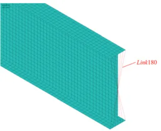
The model MT-4 is identical to MT-3 in all aspects but one: in MT-4 additional truss elements (LINK180) were added at both

supports connecting each node of the cross section to the node at the centroid of the steel section (Figure 8). The purpose of this

stiffening is to reduce or eliminate distortion of the steel section at the supports. The loads were applied as in MT-1 (Figure 6). To evaluate the influence of the position of the longitudinal support (z direction) the model MT-5 was given the same boundary conditions as MT-4, with the exception that the position of the

UZ=0 restriction was moved from the node at the bottom of the steel section to the node at its centroid (Figure 9). The loads were

applied as in MT-1 (Figure 6).

The approach adopted to apply the bending moment at the extremities

was also studied. In model 6 (same boundary conditions as

MT-5) the magnitude of the axial nodal forces applied at the end of the beam varied linearly with the depth of the section (Figure 10). This

force distribution generates a stress pattern that matches the elastic stress diagram of beams undergoing bending. This triangular force

distribution replaces the force binary at the flanges previously adopted

to introduce the bending moment, but the uniformly distributed

transversal loads were applied as described for MT-1.

Model MT-7 has the same boundary conditions as MT-1 but the

bending moment at the extremity was applied using the triangular

force diagram described for MT-6 (Figure 10).

In models MT-1 through MT-7 the bending moment was applied at

a single extremity. In order to simulate an internal span the model

MT-8 was created with the same boundary conditions and load introduction approach as MT-1 (Figure 6), the only difference being that the bending moment was applied at both extremities. Model MT-9 has the same boundary condition configuration as MT-1, but

the bending moment was applied at both extremities using the

elastic triangular diagram described for MT-6 (Figure 10). Finally, model MT-10 is a copy of model MT-6 with bending moment

applied at both ends.

Table 3 compiles the characteristics of the numerical models

MT-1 through MT-10 used in the study of boundary conditions

performed in this paper. Table 4 displays the numerical results

λANSYS (eigenvalues of the linear buckling analysis) along with the buckling mode observed (LWB stands for local web buckling). The

reference values were taken from MT-1 for models with bending moment at a single end and from MT-8 for models with bending

moment at both ends. The ratios between the eigenvalues of the reference model (λ_REF) and the eigenvalues of each model (λ_ANSYS) are also presented in Table 4.

From Table 4 the importance of the introduction of some form of

restriction against distortion at the supports (either web stiffeners

or LINK180 truss elements) becomes clear, since models without such restriction displayed the local phenomenon of web buckling instead of the global phenomenon of lateral-distortional buckling.

Figure 8

Boundary conditions in model MT-4

Figure 9

Boundary conditions in model MT-5

Figure 10

The buckling modes obtained for MT-2 and MT-3 were LWB

and an interaction between LWB and LDB, respectively, neither

of interest to this study. Comparing models MT-4 and MT-1 it is possible to conclude that the presence of the web stiffener does

not compromise the free warping behavior of the fork support,

since the difference between the eigenvalues was of 1%.

With respect to the position of the vertical and longitudinal supports, Table 4 shows that placing the restriction either at the centroid or at

the bottom flange (models MT-1 and MT-5) does not significantly alter the results (difference of 1% between the eigenvalues).

Therefore the fact that the cross sections at the supports pivot

around either the centroid or the bottom flange does not influence

the results and either approach can be adopted.

When comparing models 1 with 7 and models 8 with

MT-9, it is possible to notice that the approach to introduce the bending moment (either the force binary or the elastic triangular force diagram)

and its consequent stress distribution did not influence the results,

since the λ_REF / λ_ANSYS ratios were equal to 1.02 and 0.99, respectively. Based on the observations that resulted from this study of the

boundary conditions it is possible to conclude that the boundary

conditions of models MT-5 and MT-10 (displacement restrictions

applied at the steel section centroid, LINK180 elements at the supports to prevent distortion, and elastic triangular force diagram to apply the bending moment) are satisfactory for the study of lateral-distortional buckling and were, therefore, adopted in the parametric analysis performed in this paper.

2.3 Description of the numerical model

For the validation of the numerical model two kinds of torsional

restriction were implemented using the spring element COMBIN14: infinite rotational stiffness (considering that the concrete slab has infinite flexural stiffness) and k

1 rotational stiffness (calculated

based on the actual flexural stiffness of the concrete slab). In

each case the elastic critical moment was obtained from the

numerical analysis (M_cr,∞ and Mcr, respectively). Table 5 displays the examples analyzed in order to validate the numerical model adopted in this paper, with the ratios k₁/k₂ and M_cr / M_cr,∞taken from

Table 3

Boundary conditions studied

Model Web stiffeners _{at supports}

Distortional restriction (Link 180)

Position of vertical support

Position of longitudinal

support

Bending moment application

MT-1 Yes No Bottom flange Bottom flange Force binary

MT-2 No No Bottom flange Bottom flange Force binary

MT-3 No No Centroid Bottom flange Force binary

MT-4 No Yes Centroid Bottom flange Force binary

MT-5 No Yes Centroid Centroid Force binary

MT-6 No Yes Centroid Centroid Elastic diagram

MT-7 Yes No Bottom flange Bottom flange Elastic diagram

MT-8 Yes No Bottom flange Bottom flange Force binary

MT-9 Yes No Bottom flange Bottom flange Elastic diagram

MT-10 No Yes Centroid Centroid Elastic diagram

Table 4

Results obtained

Model λ_ANSYS λ_Reference/λ_ANSYS Buckling mode

MT1 54.9362 – LDB

MT2 20.2109 2.72 LWB at support

MT3 45.3439 1.21 LDB + LWB at support

MT4 55.5789 0.99 LDB

MT5 55.5789 0.99 LDB

MT6 54.6327 1.01 LDB

MT7 53.9052 1.02 LDB

MT8 9.77831 – LDB

MT9 9.79843 0.99 LDB

the graphics presented by Chen and Wang [4]. The slab stiffness

k₁ was calculated based on the ratios k₁/k₂ described by Chen and

Wang [4], given that the stiffness of the steel web (k2) is equal to 70,08 kNm/m, as determined by Equation 8.

From the graphics in Figure 11 it can be noted that the results of the numerical model present similar behavior to the one obtained by Chen and Wang [4]. The values display a maximum deviation

of 4% for models with L/d ratio equal to 8 (Table 5) and of 10% for

models with L/d ratio equal to 12 (Table 5).

Given the results comparison presented it can be concluded that the numerical model adopted in this work is validated and proved itself accurate in the determination of the elastic critical moment associated with lateral-distortional buckling.

3. Parametric study

In the parametric study the boundary conditions of the numerical

model were altered. The simply supported span (simplified model

proposed by Roik, Hanswille and Kina [8]) was simulated, along with models with either two or three spans, representing end and internal composite beam spans. The boundary conditions for a single simply supported span are described in item 2.2. For models with two or three spans the boundary conditions are similar to those of the simply supported beams: all supports restrict vertical displacement and a single support prevents longitudinal displacement.

The steel-concrete composite section represented in Figure 12-a was adopted and the lateral-distortional buckling was studied in

this paper using the simplified numerical model of Figure 12-b. To obtain the value of the slab stiffness k1 Equation 7 was applied considering an edge beam (that is, a equals 2) and the distance

between adjacent parallel beams (a) equal to 200 cm; the flexural stiffness of the homogenized composite section, discarding the

concrete under tension, was equal to 528 kNm, resulting in k₁ equal to 528 kN/rad. The length of the span (L) was equal to 1500 cm, approximately 25 times the depth of the beam. The factor related to the geometry of the cross section of the composite beam (α_g) was

Table 5

Results obtained by Chen and Wang [4] and numerical results obtained in this work

a) ratio L/d = 8

Chen and Wang (2012) Numerical results

k₁/k₂ k₁ M_cr/M_cr,∞ M_cr/M_cr,∞ Relative deviation (%)

0 0 0.808 0.839 4%

0.90 62.87 0.880 0.871 -1%

2.93 205.46 0.931 0.910 -2%

4.97 348.25 0.949 0.931 -2%

6.92 484.84 0.964 0.944 -2%

9.93 696.01 0.976 0.956 -2%

11.97 838.91 0.976 0.962 -1%

14.90 1043.92 0.979 0.983 0%

29.88 2093.85 0.991 0.982 -1%

49.91 3497.99 0.991 0.989 0%

b) ratio L/d = 12

Chen and Wang (2012) Numerical results

k₁/k₂ k₁ M_cr/M_cr,∞ M_cr/M_cr,∞ Relative deviation (%)

0 0 0.484 0.530 9%

1.02 75.09 0.697 0.642 -9%

2.98 219.01 0.833 0.754 -10%

5.02 369.19 0.885 0.814 -9%

6.97 513.11 0.914 0.850 -8%

9.95 732.12 0.937 0.883 -6%

11.99 882.29 0.946 0.899 -5%

14.97 1101.30 0.955 0.915 -4%

29.93 2202.61 0.979 0.954 -3%

equal to 1.09. Torsional stiffness, G_aJ, was equal to 143617 kNcm². The elastic modulus of the steel was equal to 20000 kN/cm² and the second moment of area of the bottom flange of the steel section

about the y axis (I_afy) was equal to 267 cm4. Finally, the ratio M cr/Cdist was equal to 5379 kNcm.

All scenarios in Table 1 and Table 2 were studied. The Table 1

beams have either uniformly distributed or point load. M0 is the maximum value of the bending moment (at the middle of the span) and though the beams were simply supported, the bending moment at the extremity is equal to yM₀, a value directly applied to simulate a continuous beam.

For the inner spans of the continuous composite beams with uniformly distributed transverse loads, three possible ratios

between the maximum sagging bending moment (M0) and the hogging bending moment at the extremities were studied: 0.5yM₀, 0.75yM₀, and yM₀.

To simulate the end span of continuous composite beams,

simplified models (consisting of a single simply supported span)

were adopted and a hogging bending moment ML was applied at the left end of the beam. The values of ML are listed in Table 6 and Table 8 (models M1 through M9 and M73 through M81). The simplified models of the inner spans were obtained in a similar manner, by applying hogging bending moments ML and MR to

the left and right ends (respectively) of a simply supported beam.

The values of ML and MR for models M10 through M26 and M82 through M90 are given in Table 6 and Table 8.

To analyze the influence of the adjacent spans a more complex

model was adopted. Beams with two spans were modeled to simulate end spans and beams with three spans were modeled to simulate inner spans. For the end spans of continuous beams with

uniformly distributed transverse load (models M37 through M45 in

Table 7) it was possible to obtain a relation between the distributed loads q₁ and q₂ by employing the three-moment equation. Taking the distributed load in the analyzed span q₂ as being equal to 1 kN/m it follows that:

(9)

Figure 11

Comparison between the numerical results obtained in this work and the results published by Chen

and Wang [4]

a) ratio L/d = 8 b) ratio L/d = 12

Figure 12

Model adopted for the numerical study

Similar analytical relations were obtained for the models containing

the inner span (M46 through M72 in Table 7) by also applying the

three-moment equation to the three possible variations of the

bending moment diagram. For the hogging moments at the ends equal to yM₀ and 0.5yM₀ the relations are:

(10)

Table 6

Numerical models of simply supported continuous composite beams with uniformly distributed

transverse load

Model Boundary conditions Bending moment _diagram y M_L (kNm) M_R (kNm)

M1 0.5 14.06 –

M2 0.75 21.09 –

M3 1 28.13 –

M4 1.25 35.16 –

M5 1.5 42.19 –

M6 1.75 49.22 –

M7 2 56.25 –

M8 2.25 63.28 –

M9 2.5 70.31 –

M10 0.5 14.06 7.03

M11 0.75 21.09 10.55

M12 1 28.13 14.06

M13 1.25 35.16 17.58

M14 1.5 42.19 21.09

M15 1.75 49.22 24.61

M16 2 56.25 28.13

M17 2.25 63.28 31.64

M18 2.5 70.31 35.16

M19 0.5 14.06 10.55

M20 0.75 21.09 15.82

M21 1 28.13 21.09

M22 1.25 35.16 26.37

M23 1.5 42.19 31.64

M24 1.75 49.22 36.91

M25 2 56.25 42.19

M26 2.25 63.28 47.46

M27 2.5 70.31 52.73

M28 0.5 14.06 14.06

M29 0.75 21.09 21.09

M30 1 28.13 28.13

M31 1.25 35.16 35.16

M32 1.5 42.19 42.19

M33 1.75 49.22 49.22

M34 2 56.25 56.25

M35 2.25 63.28 63.28

₍₁₁₎

For bending moments at the end of the analyzed span equal

to yM₀ and 0.75yM₀ the relations become:

(12)

Table 7

Numerical models with two or three spans of continuous composite beams with uniformly distributed

transverse load

Model Boundary conditions Bending moment _diagram y q₁ (kN/m) q₂ (kN/m)

M37 0.5 0 –

M38 0.75 0.50 –

M39 1 1.00 –

M40 1.25 1.50 –

M41 1.5 2.00 –

M42 1.75 2.50 –

M43 2 3.00 –

M44 2.25 3.50 –

M45 2.5 4.00 –

M46 0.5 0.13 -0.25

M47 0.75 0.69 0.13

M48 1 1.25 0.5

M49 1.25 1.81 0.88

M50 1.5 2.38 1.25

M51 1.75 2.94 1.63

M52 2 3.50 2

M53 2.25 4.06 2.38

M54 2.5 4.63 2.75

M55 0.5 0.19 0

M56 0.75 0.78 0.5

M57 1 1.38 1

M58 1.25 1.97 1.5

M59 1.5 2.56 2

M60 1.75 3.16 2.5

M61 2 3.75 3

M62 2.25 4.34 3.5

M63 2.5 4.94 4

M64 0.5 0.25 0.25

M65 0.75 0.88 0.88

M66 1 1.50 1.5

M67 1.25 2.13 2.13

M68 1.5 2.75 2.75

M69 1.75 3.38 3.38

M70 2 4 4

M71 2.25 4.63 4.63

Table 8

Numerical models of simply supported continuous composite beams with point load

Model Boundary conditions Bending moment

diagram y ML (kN/m) MR (kN/m)

M73 0.5 1.88 –

M74 0.75 2.81 –

M75 1 3.75 –

M76 1.25 4.69 –

M77 1.5 5.63 –

M78 1.75 6.56 –

M79 2 7.50 –

M80 2.25 8.44 –

M81 2.5 9.38 –

M82 0.5 1.88 1.88

M83 0.75 2.81 2.81

M84 1 3.75 3.75

M85 1.25 4.69 4.69

M86 1.5 5.63 5.63

M87 1.75 6.56 6.56

M88 2 7.50 7.50

M89 2.25 8.44 8.44

M90 2.5 9.38 9.38

Table 9

Numerical models of continuous composite beams with two or three spans with point loads

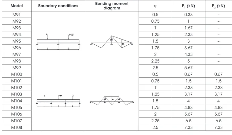
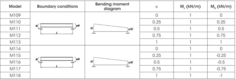
Model Boundary conditions Bending moment _diagram y P₁ (kN) P₂ (kN)

M91 0.5 0.33 –

M92 0.75 1 –

M93 1 1.67 –

M94 1.25 2.33 –

M95 1.5 3 –

M96 1.75 3.67 –

M97 2 4.33 –

M98 2.25 5 –

M99 2.5 5.67 –

M100 0.5 0.67 0.67

M101 0.75 1.5 1.5

M102 1 2.33 2.33

M103 1.25 3.17 3.17

M104 1.5 4 4

M105 1.75 4.83 4.83

M106 2 5.67 5.67

M107 2.25 6.5 6.5

(13)

Finally, when the hogging moment at both ends is equal to yM₀ the relation becomes:

(14)

For continuous composite beams with point loads (models M91 through M99 in Table 9) the three-moment equation was also

applied and the relation between the point loads P₁ and P₂ is given by Equation 15:

(15)

For the models with the inner span (M100 through M108 in Table

9), the relations between the point loads P₁, P₂ and P₃ were:

(16)

The beams in Table 2 do not have transverse load applied along the length of the span (L), only hogging moments applied at the ends of the span, which causes the bending moment diagram to

display a linear shape. For these cases only the simplified models

(a single simply supported span with bending moments applied at

the ends) were simulated. For models M109 through M113 in Table 10 a bending moment M of 1kNm was applied to the left end and a

bending moment equal to yM was applied at the right end in order to produce a bending moment diagram with a trapezoidal shape.

4. Analysis of the results

4.1 Numerical models of composite beams

with uniformly distributed transverse load

Table 11 presents the results obtained numerically for the simplified models (M1 through M36) and for the models with more than one span (M37 through M72) with distributed transverse load. The results obtained for the simplified models (Mcr,s) and for the models

with more than one span (Mcr,v) are confronted with the values obtained by applying Equation 1, proposed by Roik, Hanswille and

Kina [8] and adopted by ABNT NBR 8800:2008 (Mcr,ABNT).

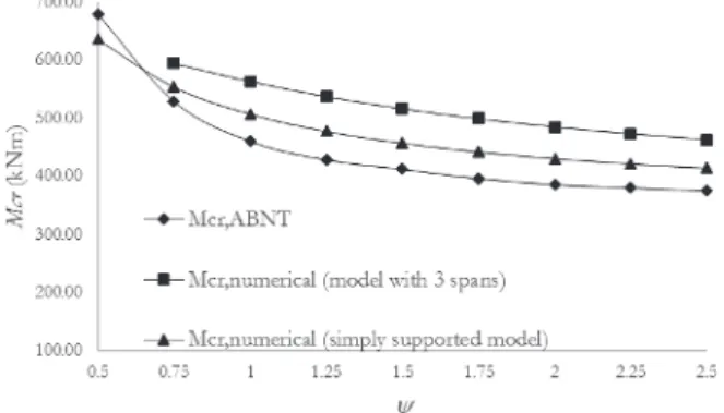
From Figure 13 it is possible to observe that the simplified model

displays the same behavioral tendency that can be generated by applying the formulation prescribed by ABNT NBR 8800:2008, i.e.,

Mcr decreases with the increase of the y factor. However, the slope of the curve obtained by implementing the ABNT NBR 8800:2008 procedure is steeper and the numerical results display lower values than the ones obtained from Equation 1.

In Figure 13 it can be noted that beams modeled with more than one span also displayed the same tendency derived from the ABNT NBR 8800:2008 procedure for y values greater than 1.0

(Mcr decreases with the increase of y). For y values below 1.0

it is not possible to analyze the Mcr obtained, since in this case the adjacent span is the one that displays the lateral-distortional buckling behavior. It is also clear that the results obtained using

the simplified model (single span) are very close to the ones

obtained modelling beams with more spans, demonstrating that

the adjacent span influences very little in the results collected from

the analyzed span. Therefore, it is possible to conclude that the

simplified numerical model displays very good accuracy.

When comparing the numerical results of the simplified models

with the values obtained by applying the ABNT NBR 8800:2008

procedure (Table 11), ratios of Mcr,s/Mcr,ABNT ranging from 0.35 to

0.65 for end spans (models M1 through M9) and from 0.43 to 1.11 for inner spans (M10 through M36) were observed. For models with more than one span (M37 through M45) the Mcr,v/Mcr,ABNT ratio ranges between 0.49 and 0.77 for end spans, meaning that ABNT NBR 8800:2008 predicts unsafe values for the elastic

critical moment. For inner spans (models M46 through M72) a

greater similarity between numerical values and analytical values

was observed, with the Mcr,v/Mcr,ABNT ratio varying between 0.71 and 1.39.

4.2 Numerical models of compositee beams

with point load

Table 10

Numerical models of simply supported continuous composite beams without loading along the

member length L

Model Boundary conditions Bending moment _diagram y M_L (kN/m) M_R (kN/m)

M109 0 1 0

M110 0.25 1 0.25

M111 0.5 1 0.5

M112 0.75 1 0.75

M113 1 1 1

M114 0 1 0

M115 0.25 1 -0.25

M116 0.5 1 -0.5

M117 0.75 1 -0.75

Table 11

Numerical and analytical results of continuous composite beams with uniformly distributed

transverse load

Models

y C_dist Mcr,ABNT

(kNm)

M_cr,s (kNm)

M_cr,v (kNm)

M_cr,s/ M_cr,ABNT

M_cr,v/ M_cr,ABNT Simplified

1 span

With 2 or 3 spans

M1 M37 0.5 41.5 2223.26 789.20 496.71 0.35 0.22

M2 M38 0.75 30.2 1617.89 715.78 642.09 0.44 0.40

M3 M39 1 24.5 1312.53 659.29 649.58 0.50 0.49

M4 M40 1.25 21.1 1130.38 619.98 646.65 0.55 0.57

M5 M41 1.5 19 1017.88 591.95 641.85 0.58 0.63

M6 M42 1.75 17.5 937.52 571.20 637.42 0.61 0.68

M7 M43 2 16.5 883.95 555.31 633.76 0.63 0.72

M8 M44 2.25 15.7 841.09 542.79 630.78 0.65 0.75

M9 M45 2.5 15.2 814.30 532.69 628.36 0.65 0.77

M10 M46 0.5 33.9 1816.11 777.62 526.19 0.43 0.29

M11 M47 0.75 22.7 1216.10 692.52 656.40 0.57 0.54

M12 M48 1 17.3 926.80 630.32 653.99 0.68 0.71

M13 M49 1.25 14.1 755.37 587.93 643.06 0.78 0.85

M14 M50 1.5 13 696.44 558.03 632.38 0.80 0.91

M15 M51 1.75 12 642.87 536.02 623.62 0.83 0.97

M16 M52 2 11.4 610.73 519.22 616.75 0.85 1.01

M17 M53 2.25 10.9 583.94 506.00 611.40 0.87 1.05

M18 M54 2.5 10.6 567.87 495.35 607.17 0.87 1.07

M19 M55 0.5 28.2 1510.75 770.93 619.86 0.51 0.41

M20 M56 0.75 18 964.31 679.83 661.59 0.70 0.69

M21 M57 1 13.7 733.94 614.75 652.72 0.84 0.89

M22 M58 1.25 11.7 626.80 570.75 637.34 0.91 1.02

M23 M59 1.5 10.6 567.87 539.77 623.43 0.95 1.10

M24 M60 1.75 10 535.73 516.96 612.26 0.96 1.14

M25 M61 2 9.5 508.94 499.53 603.66 0.98 1.19

M26 M62 2.25 9.1 487.51 485.81 597.00 1.00 1.22

M27 M63 2.5 8.9 476.80 474.75 591.75 1.00 1.24

M28 M64 0.5 21.9 1173.24 760.93 631.82 0.65 0.54

M29 M65 0.75 13.9 744.66 666.41 664.87 0.89 0.89

M30 M66 1 11 589.30 596.53 647.70 1.01 1.10

M31 M67 1.25 9.6 514.30 548.51 625.86 1.07 1.22

M32 M68 1.5 8.8 471.44 514.93 607.51 1.09 1.29

M33 M69 1.75 8.3 444.65 490.43 593.63 1.10 1.34

M34 M70 2 8 428.58 471.84 583.22 1.10 1.36

M35 M71 2.25 7.8 417.87 457.31 574.93 1.09 1.38

M36 M72 2.5 7.6 407.15 445.65 567.73 1.09 1.39

Figure 13

M

x

y

for continuous composite beams with uniformly distributed load

a) end span models (M1 through M9 and M37 through M45) b) inner span models (M10 through M18 and M46 through M54)

c) inner span models (M19 through M27 and M55 through M63) d) inner span models (M28 through M36 and M64 through M72)

Table 12

Numerical and analytical results of continuous composite beams with point loads

Models

y C_dist Mcr,ABNT

(kNm)

M_cr,s (kNm)

M_cr,v (kNm)

M_cr,s/ M_cr,ABNT

M_cr,v/ M_cr,ABNT Simplified

1 span

With 2 or 3 spans

M73 M91 0.5 28.4 1521.46 687.29 582.41 0.45 0.38

M74 M92 0.75 21.8 1167.88 617.80 609.90 0.53 0.52

M75 M93 1 18.6 996.45 577.94 602.99 0.58 0.61

M76 M94 1.25 16.7 894.66 552.58 592.30 0.62 0.66

M77 M95 1.5 15.6 835.73 535.10 582.52 0.64 0.70

M78 M96 1.75 14.8 792.87 522.33 622.65 0.66 0.79

M79 M97 2 14.2 760.73 512.60 567.22 0.67 0.75

M80 M98 2.25 13.8 739.30 504.93 561.33 0.68 0.76

M81 M99 2.5 13.5 723.23 498.74 556.33 0.69 0.77

M82 M100 0.5 12.7 680.37 636.42 617.16 0.94 0.91

M83 M101 0.75 9.89 529.83 554.48 595.37 1.05 1.12

M84 M102 1 8.6 460.72 507.39 563.68 1.10 1.22

M85 M103 1.25 8 428.58 477.59 537.51 1.11 1.25

M86 M104 1.5 7.7 412.51 457.03 516.42 1.11 1.25

M87 M105 1.75 7.4 396.44 441.96 499.16 1.11 1.26

M88 M106 2 7.2 385.72 430.42 484.87 1.12 1.26

M89 M107 2.25 7.1 380.36 421.29 472.93 1.11 1.24

M90 M108 2.5 7 375.01 413.88 462.90 1.10 1.23

Table 12 displays the results obtained numerically for the simplified models (M73 through M90) and for the models with more than one span (M91 through M108) with point loads. The results obtained for the simplified models (Mcr,s) and for the models with more than one

span (Mcr,v) were confronted against those obtained by applying

Equation 1 (Mcr,ABNT).

From Figure 14-a it is possible to observe that the numerical

models, both the simplified and those with more than a single

span, displayed the same overall behavior detected in the models with distributed load (Figure 13-a). Figure 14-b shows that for all values of y the numerical results are higher than those obtained by applying the ABNT NBR 8800:2008 procedure.

When comparing the numerical results of the simplified models against the ABNT NBR 8800:2008 results (Table 12), ratios of Mcr,s/

Mcr,ABNT ranging from 0.45 to 0.69 for end spans (M73 through M81)

and from 0.94 to 1.11 for inner spans (M82 through M90) were observed. For models with more than one span (M91 through M99) the Mcr,v/Mcr,ABNT ratio ranges between 0.38 and 0.79 for end spans,

meaning that yet again ABNT NBR8800:2008 predicts unsafe

values for the elastic critical moment Mcr. For inner spans (models

M100 through M108) a greater similarity between numerical values and analytical values was observed, with the Mcr,v/Mcr,ABNT ratio varying between 1.12 and 1.26, always predicting safe values.

4.3 Numerical models of composite beams

without transverse loads

Table 13 presents the results obtained numerically for the

simplified models with hogging moments at the ends causing a single curvature (M109 through M113) and for the models with bending moments at the ends generating a double curvature (M91 through M108). The results obtained using the simply supported model (Mcr,b) were confronted with the ones obtained by applying

the procedure prescribed by ABNT NBR 8800:2008 (Mcr,ABNT). From Figure 15 it can be noted that the simply supported model displays the same behavioral tendency than can be generated

Figure 14

M

x

y

for continuous composite beams with point loads

a) end span models (M73 through M81 and M91 through M99) b) inner span models (M82 through M90 and M100 through M108)

Table 13

Numerical and analytical results of continuous composite beams without loading along the member

length L

Models

y C_dist Mcr,ABNT

(kNm)

M_cr,b

(kNm) Mcr,b/ Mcr,ABNT

Simply supported

M109 0 11.1 594.66 440.29 0.74

M110 0.25 9.5 508.94 420.20 0.83

M111 0.5 8.2 439.29 398.70 0.91

M112 0.75 7.1 380.36 375.05 0.99

M113 1 6.2 332.15 344.77 1.04

M114 0 11.1 594.66 440.29 0.74

M115 0.25 12.8 685.73 459.41 0.67

M116 0.5 14.6 782.16 477.81 0.61

M117 0.75 16.3 873.23 495.66 0.57

M118 1 18.1 969.66 513.03 0.53

by applying the ABNT NBR8800:2008 method, i.e., M

cr decreases with the increase of the y factor. However, the slope of the curves

associated with Mcr,ABNT is steeper than the one associated with the numerical results. The numerical model returns values that are inferior to those obtained by applying Equation 1 in all cases but the one in which there is single curvature and y is greater than 0.5.

From Table 13 the Mcr,s/Mcr,ABNT ratio can be seen ranging from

0.74 to 1.04 (models M109 through M113, single curvature) and from 0.53 to 0.74 (models M114 through M118, double curvature),

leading to the conclusion that ABNT NBR 8800:2008 predicts

unsafe values for Mcr (except for beams with a single curvature

when ψ is greater than 0.5).

4.4 Proposed values for the modification parameter

Previous discussion in items 4.1 through 4.3 showed there was

a small difference between the simplified models and the models

with more than one span. Since models with multiple spans more accurately simulate the behavior of continuous composite beams, the use of Table 14 and Table 15 is suggested in place of Table 1 and Table 2 from ABNT NBR 8800:2008 in order to determine the values of the C_dist coefficient. The C_dist values in Table 14 and Table 15 were obtained based on the numerical results by applying Equation 17.

(17)

in which M_cr is the value of the elastic critical moment obtained using the numerical models with more than one span, if y is equal to or greater than 1, and using the numerical models with a single

Figure 15

M

x

y

for continuous composite beams without loads along member length L

a) models with single curvature (M109 through M113)

b) models with double curvature (M114 through M118)

Table 14

Proposed values of C

for spans with uniformly distributed or point loads

Loading and boundary conditions

Bending moment diagram1

C_dist

y=0.50 y=0.75 y=1.00 y=1.25 y=1.50 y=1.75 y=2.00 y=2.25 y=2.50

Mo Mo

y

14.7 13.4 12.1 12.1 12.0 11.9 11.8 11.8 11.7

Mo Mo

y 0.50 Myo _{14.5 12.9 12.2 12.0 11.8 11.6 11.5 11.4 11.3}

Mo Mo

y 0.75 Myo

14.4 12.7 12.2 11.9 11.6 11.4 11.3 11.1 11.0

Mo Mo

y y_Mo

14.2 12.4 12.1 11.7 11.3 11.1 10.9 10.7 10.6

y_Mo Mo

12.8 11.5 11.3 11.1 10.9 11.6 10.6 10.5 10.4

Mo Mo y Mo

y _{11.9 11.1 10.5 10.0 9.6 9.3 9.1 8.8 8.6}

Note:1_M

simply supported span if y is smaller than 1.

5. Conclusion

In this paper, numerical models were developed in the finite

element software Ansys to simulate the lateral-distortional buckling behavior of continuous steel-concrete composite beams and

determine the elastic critical moment. The different boundary

conditions presented in ABNT NBR 8800:2008 were replicated

in simplified models with a single simply supported span and in

more complex models with more than one span, which made it

possible to evaluate the modification parameter Cdist. The influence of the bending moment distribution was analyzed and ultimately led to the conclusion that the formulation proposed by ABNT NBR 8800:2008 might lead to unsafe predictions.

This paper proposes new values for the modification parameter

C_dist based on the numerical results obtained for models with more than a single span and a y value greater than 1. Since in models with more than one span it is not possible to analyze the cases in which y is smaller than 1, the C_dist obtained in the simplified numerical model (single simply supported span) was used. The observation was made that, for continuous composite beams, the bending moment distribution along the length of the span

influences very little the resulting Mcr value, given that the Cdist values are nearly constant. A revision of the C_dist values proposed by ABNT NBR 8800:2008 is recommended based on the C_dist values obtained numerically in this paper.

6. Acknowledgments

The authors acknowledge the support provided by the Brazilian

public agencies CNPq, CAPES, FAPES and FAPEMIG in the

development of this research.

7. References

[1] Ansys, INC., 2011. Release 15.0 Documentation for ANSYS. Canonsburg: [s.n.].

[2] Associação Brasileira de Normas Técnicas – ABNT. ABNT NBR 8800:2008Projeto de estrutura de aço e de estrutura

mista de aço e concreto de edifícios. Rio de Janeiro.

[3] Calenzani, A.F.G., Fakury, R.H., Paula, F.A., Rodrigues, F.C.,

Queiroz, G. & Pimenta, R.J., 2012. Rotational stiffness of continuous composite beams with sinusoidal-web profiles for torsional buckling.Journal of Constructional Steel Research,

n.79, p. 22-33.

[4] CEN, EN 1994-1-1:2004. Eurocode4:Design of composite steel and concrete structures - Part 1-1: general rules and rules for buildings. Bruxelas, Bélgica.

[5] Chen, S. & Wang, X., 2012.Finite Element Analysis of Distortional Lateral Buckling of Continuous Composite

Beams with Transverse Web Stiffeners.Advances in

Structural Engineering, vol. 15, pp. 1607-1616.

[6] Ng, M.L.H. &Ronagh, H.R., 2004. An analytical solution for

the elastic lateral-distortional buckling of I-section beams. Advances in Structural Engineering, vol. 7, p. 189-200.

[7] Oliveira, J.P.S., 2014. Determinação do momento crítico de flambagem lateral com distorção em vigas mistas contínuas de aço e concreto com perfis de alma senoidal. Dissertação,

Universidade Federal do Espírito Santo, Vitória.

[8] Roik, K., Hanswille, G. & Kina, J., 1990.Solution for the

lateral torsional buckling problem of composite beams.

Stahlbau, n-59, 327 – 332 (em alemão).

Table 15

Proposed values of C

for spans without loads along the member length L

Loading and boundary conditions

Bending moment diagram1

C_dist

y=0.00 y=0.25 y=0.50 y=0.75 y=1.00

M ÈM

acceptable 8.2 7.8 7.4 7.0 6.4

M

ÈM

acceptable 8.2 8.6 8.9 9.3 9.6

Note:1_{M is the maximum design hogging moment, in absolute value, at the analyzed span, considering that y values grater than 1.00 have to be}