M
ASTER
M
ATHEMATICAL
F
INANCE
M
ASTERS
F
INAL
W
ORK
I
NTERNSHIP
R
EPORT
D
ETERMINATION ANDA
NALYSIS OFPRIIP
P
ERFORMANCES
CENARIOSP
EDROL
EANDROA
NTUNESB
ARROSM
ASTER
M
ATHEMATICAL
F
INANCE
M
ASTERS
F
INAL
W
ORK
I
NTERNSHIP
R
EPORT
D
ETERMINATION ANDA
NALYSIS OFPRIIP
P
ERFORMANCES
CENARIOSP
EDROL
EANDROA
NTUNESB
ARROSSUPERVISION:
MARIA DE FÁTIMA DANTAS PIRES LIMA DR. LURDES DIOGO
iii
Acknowledgments
I want to thank my family for always being there for me, for guiding me and always giving me every chance to do better for myself.
To everyone at Caixa Geral de Depósitos for the opportunity given. It has been a pleasure being a part of such an amazing institution.
To Professor Fátima Pires Lima for the support and advice throughout the writing of this report.
iv
Abstract
The crescent number of non-professional investors taking positions on complicated financial products has led the European Union (EU) to adopt regulations about how packaged retail and insurance-based investment products (PRIIPs) must be presented to their potential buyers and aid them in making informed investment decisions through comparison amongst a diverse supply of products. These regulations – No 1286/2014 of the European Parliament and of the Council and its supplement, the Commission Delegated Regulation 2017/653 – present rules on how to assess key pieces of information about the products’ types market risk-wise, their risk levels, performance expectations, cost profiles and how to provide all these metrics in a single document – the Key Information Document (KID) – to insure that the institutions that sell investment products act on behalf of the investors’ best interests.
Foreign Exchange (FOREX, FX) products, financial instruments that allow two counterparties to acquire or dispose of positions on foreign currency, fall in the scope of the aforementioned regulations. Every time a non-professional investor wishes to have a long or short position on a currency of their choice for any reason, the bank must provide them with the KID of the product that best suits their interest. The KID must be generated and updated for each according to: the currency pair being traded; the data that serves as a base for market risk, performances and cost calculations; the maximum tenor of the deal; and what currency from the pair is being purchased or sold.
This report carries out the study and analysis of the KID’s content referring to Foreign Exchange products’ performances under four different scenarios: stress, unfavorable, moderate and favorable.
Keywords:
PRIIP, KID, Foreign Exchange Market, Market Risk, Performancev
Abbreviations
CGD – Caixa Geral de Depósitos EBA – European Banking Authority ECB – European Central Bank
EIOPA – European Insurance and Occupational Pensions Authority ESAs – European Supervisory Authorities
ESMA – European Securities and Markets Authority EU – European Union
FOREX, FX – Foreign Exchange FOREX, FX – Foreign Exchange KID – Key Information Document
MiFID II – Markets in Financial Instruments Directive II (Directive 2014/65/EU) MRM – Market Risk Measure
PRIIPs – Packaged Retail and Insurance-based Investment Products RHP – Recommended Holding Period
vi
Contents
1. Introduction ... 9
2. Literature Review ... 11
2.1. Foreign Exchange Market ... 11
2.1.1. Foreign Exchange Risk ... 11
2.1.2. Quotation Methods ... 12
2.1.3. Bid-Offer Exchange Rates... 13
2.2. Foreign Exchange Products ... 13
2.2.1. FX Spot ... 14
2.2.2. FX Forward ... 14
2.2.3. FX SWAP ... 16
2.3. Market Risk ... 18
2.3.1. VaR – Value at Risk ... 18
2.4. PRIIPs Regulation ... 19
2.4.1. PRIIPs Categories ... 19
2.4.2. Market Risk Measure ... 20
2.4.3. Performance Scenarios ... 21
3. Methodology ... 23
3.1. Regulation 2017/653’s Methodology ... 23
3.2. European Supervisory Authorities’ (ESAs) Joint Committee Methodology ... 27
3.3. Application to FX Products ... 28 4. Results ... 34 5. Conclusion ... 37 6. References ... 38 7. Appendices ... 40 A. FX Spot Cash-Flows ... 40 B. FX Forward Cash-Flows ... 41
vii
C. FX SWAP Cash-Flows... 42
D. Performance Scenarios of 7 third-party FIs ... 43
E. Forward exchange rates calculations ... 44
F. Spot vs. Forward rates’ comparison ... 45
G. Performance Scenarios of FX Forwards using Regulation 2017/653’s and ESAs’ methodologies ... 47
viii
List of Figures
Figure 1 - FX spot cash-flows diagram ... 40
Figure 2 - FX Forward cash-flows diagram ... 41
Figure 3 - FX SWAP cash-flows diagram ... 42
Figure 4 - EUR/USD exchange rates from May 27th 2014 to May 28th 2019 ... 45
Figure 5 - EUR/USD exchange rates from May 14th 2014 to May 15th 2019 ... 45
Figure 6 - EUR/USD exchange rates from April 10th 2013 to April 11th 2018 ... 45
Figure 7 - EUR/USD exchange rates from January 6th 2014 to January 7th 2019 ... 45
Figure 8 - EUR/USD exchange rates from February 5th 2014 to February 6th 2019 ... 45
Figure 9 - EUR/GBP exchange rates from May 27th 2014 to May 28th 2019 ... 45
Figure 10 - EUR/GBP exchange rates from April 10th 2013 to April 11th 2018 ... 46
Figure 11 - EUR/GBP exchange rates from January 6th 2014 to January 7th 2019 ... 46
Figure 12 - EUR/GBP exchange rates from February 5th 2014 to February 6th 2019 ... 46
Figure 13 - EUR/JPY exchange rates from May 27th 2014 to May 28th 2019 ... 46
Figure 14 - EUR/JPY exchange rates from April 10th 2013 to April 11th 2018 ... 46
Figure 15 - EUR/JPY exchange rates from February 5th 2014 to February 6th 2019 ... 46
List of Tables
Table I - Source: point 10a), Annex IV, Regulation 2017/653 ... 25Table II - Performance scenarios of third-party Financial Institutions ... 43
Table III - Forward exchange rates’ calculations for EUR/USD from May 27th 2014 to May 28th 2019 ... 44
Table IV - Approaches for EUR/USD forward exchange rates' calculations from May 27th 2014 to May 28th 2019 ... 44
Table V – Performance Scenarios using Regulation 2017/653’s methodology ... 47
9
1. Introduction
This report, part of the requirement to complete the master’s degree in Mathematical Finance by ISEG, is the product of a 3-month internship at Caixa Geral de Depósitos S.A in the Department of Market Risk Management.
Whether it be to pay for their children’s education, buy a house or secure their retirement, consumers may choose to save money by investing in certain financial investment products. Such products, the packaged retail and insurance-based investment products (PRIIPs), comprise most of the retail investment market and, despite offering potential benefits to retail investors, they can be complex and complicated for the average consumer to fully understand their behavior. This makes it hard for the non-professional investors to compare different investment products and grasp how risky they are and the potential profit or loss they might incur in by investing in a certain product.
Since the institutions that sell PRIIPs are the ones to usually advise the buyers, in order to protect the investors from the possibility of the selling institution not acting on behalf of their best interests, the European Union (EU) adopted a regulation about PRIIPs transactions. From this effort to ensure transparency in this type of transactions, emerged the obligation for the producers or sellers of investment products to provide Key Information Documents (KIDs) to potential investors.
Each KID must be produced for a specific type of product and include key pieces of information about the product and its seller, such as: the product’s description; its level of risk, from the least risky to the riskiest; its performance under stress, unfavorable, moderate and favorable scenarios for the recommended holding period and, when applicable, for any intermediate periods; information about the outcome resulting from the product’s manufacturer not being able to pay the investor; the costs associated with its purchase; how long should the investor hold the product; the platform through which the investor can file a complaint; and other information the manufacturer or seller might deem to be important.
CGD’s Risk Management Department is responsible for elaborating KID’s for the products the bank sells, in particular foreign exchange products.
10
Foreign Exchange (FOREX, FX) products, financial instruments that allow two counterparties to acquire or dispose of positions on foreign currency, fall in the scope of the aforementioned regulations. Every time a non-professional investor wishes to have a long or short position on a currency of their choice for any reason, the bank must provide them with the KID of the product that best suits their interest. The KID must be generated and updated for each according to: the currency pair being traded; the data that serves as a base for market risk, performances and cost calculations; the maximum tenor of the deal; and what currency from the pair is being purchased or sold.
This report focuses on the task for which I was responsible during the internship: the development of a model to evaluate performance scenarios of foreign exchange products under the PRIIP’s regulation. This report follows the Regulation 2017/653’s methodology and the European Supervisory Authorities’ (ESAs) interpretation of the Regulation’s methodology regarding performance scenarios, which guide the PRIIP seller through the reward calculations concerning the performance of foreign exchange products, specifically forwards and SWAPs, under four different scenarios – stress, unfavorable, moderate and favorable. Both methodologies were used as an effort to understand how differences in the Regulation’s rules interpretation may impact predictions of products’ future performances.
FX forwards and SWAPs are products that fall under a category of PRIIPs in which three of the four performance scenarios – unfavorable, moderate and favorable – are computed the same way as the market risk metric and by using the value-at-risk (VaR) measure. In order to achieve understandable results, one needs to get a grasp at the concepts they entail such as market risk and value-at-risk and how to approach the formulas presented in the regulations. The stress scenario, despite also being the VaR of the PRIIP with a certain level of confidence, employs a methodology of its own built on the concept of stress volatility of historical returns.
Performance scenarios will be computed for FX products referring to 3 currency pairs with different deal dates and the results obtained from this report’s interpretation of the Regulation 2017/653’s methodology will be compared with the ones from third-party Financial Institutions (FIs) and from the ESAs’ methodology and will lead a conclusion about the topic.
11
2. Literature Review
2.1. Foreign Exchange Market
Silva et al. (2016) defines the Foreign Exchange (FOREX/FX) Market as a global, decentralized and over-the-counter market where currencies are traded in the form of financial instruments and may be held for different intents such as speculation (highly risky strategy for investors seeking to profit from other financial instruments’ prices variations), arbitrage (simultaneous buying and selling of a financial instrument in different markets to profit from price disparities) or commercial transaction purposes.
Shamah (2003) simply puts it as the unregulated process of buying a currency and selling another, always doing so in pairs.
The following example illustrates how an FX operation may help with a business transaction: suppose a Portuguese company wants to import goods from America and their price is expressed in Dollars. The company will need to acquire Dollars in order to pay for the goods and will do so by selling their Euros. The price for such operation is the exchange rate: the price at which a currency is traded for another (Sercu 2008).
Hedging the currency risk may also be the purpose of taking a long/short position in FX products if their buyer/seller wants the exchange to occur in the future. The elimination of the uncertainty that the foreign currency weakens against the base currency or the base currency strengthens against the foreign currency is an important factor for many small businesses when trying to protect themselves from massive losses when trading in a foreign currency due to its high volatility.
2.1.1. Foreign Exchange Risk
According to (Silva et al. 2016) and (Shamah 2003) it’s common to classify the foreign exchange exposure in three types: transaction exposure, translation exposure and economic exposure. These exposures originate the risk of a financial impact on the company due to any changes in foreign exchange rates.
The transaction exposure is the one more intuitive as it impacts companies’ inflows and outflows of cash-flows and, consequently, its profits and losses. It measures
12
the risk of a currency rate fluctuation after a company takes over the financial obligation to pay/receive a future bill on a foreign currency.
The translation exposure (also known as accounting exposure) is the risk of a company’s value change as a consequence of a currency rate fluctuation of its assets and/or liabilities.
The economic exposure concerns a company’s vulnerability to foreign markets and their suppliers. It can be verified when different companies compete in the same market and their respective values are impacted by changes in the exchange rate that applies to them.
In order to mitigate or fully eliminate these exposures, thus getting rid of foreign exchange risk altogether, one can enter different available contracts that best suits them. Amongst these contracts, the ones I will go back to are spot transactions, forward transactions and swap transactions.
2.1.2. Quotation Methods
There are two different methods for quoting a currency in terms of another:
• Direct quotation – measure the value of one unit of foreign currency in
terms of the base currency. The base currency is the quoted one.
• Indirect quotation – is the reciprocal of the direct quotation and measured
the value of one unit of a base currency in terms of a foreign currency. The euro currency, as well as the British pound and Australian dollar, are generally quoted in indirect form. For example EUR/USD and GBP/USD, which refers to the amount of US dollars per one euro and one British pound, respectively).
Considering the Eurodollar exchange rate, which is quoted indirectly, the Euro is the base currency and the US Dollar is the foreign currency so, having X EUR/USD means that X units of US Dollars will buy 1 Euro.
13
2.1.3. Bid-Offer Exchange Rates
For a specific currency pair there are two exchange rates: one for buying and another for selling currencies. A financial entity may be willing to buy a foreign currency for a price that is different from the one they are willing to sell the base currency for:
• Bid price is the price, in terms of the base currency, the financial institution
is willing to pay to receive the foreign currency (accept to sell the base currency);
• Ask price is the price, in terms of the foreign currency, the financial
institution is willing to pay to receive the base currency (accept to sell the foreign currency);
The difference between the bid and the ask prices is the spread and represents the institution’s profit (margin) for engaging in the two trades.
2.2. Foreign Exchange Products
In order to negotiate in the foreign exchange market, one can choose one of three traditional ways to do so, according to their needs: spot, forward and swap transactions (Silva et al. 2016). Any of these operations consist of agreements in which the counterparties are obliged to trade a currency pair at a determined price and at a specific settlement date.
It’s important to emphasize that only forward and swap transactions incorporate a hedging factor underlying to the transaction itself since the counterparty interested in acquiring currency in a future settlement date is given the chance to do it at a more favorable exchange rate rather than the spot one. When entering a spot transaction, the acquirer simply negotiates at the spot exchange rate without the possibility of hedging against unfavorable rate movements.
Any FX transaction may be used to hedge against unfavorable exchange rate movements if the acquirer owns FIs measured in a foreign currency and wants to guarantee that they eliminate the uncertainty of incurring in loses in the future when alienating such FIs.
14
2.2.1. FX Spot
A foreign exchange spot transaction, also known as FX spot, is a transaction in which a currency is exchanged for another with settlement date in two business days.
The rate used in this operation is called the spot rate and expresses the price of one currency in terms of another at the deal date for delivery in the settlement date.
For this type of transaction, the financial institution buys currency at the bid rate and sells it at the ask rate, earning the difference. This difference reflects also the currency’s liquidity: the smaller the spread, the more liquid the currency.
Although the Bank of Portugal discloses daily spot exchange rates, this value is just for reference; the authorized financial institution may trade currency at the spot rate they intent to, making they effectively market-makers (Silva et al. 2016).
As can be observed in Figure 1’s illustration of the cash-flows involved in one FX spot financial operation, a spot deal is useful when the counterparty taking a long or short position in foreign currency benefits from it.
2.2.2. FX Forward
An FX forward contracts is a FX spot contract with a delivery date longer than the spot’s two business days.
At a first glance, it would be reasonable to assume that the rate used for the spot transactions apply to the forward ones, but such reasoning lacks scope about how a currency’s value may change in the future. In fact, since the exchange rates used for forward operations are stablished for a future date, it’s only natural to incorporate future expectations about a currency’s value in the forward rate’s value, which in turn may be bigger or smaller than the original spot rate (Silva et al. 2016). Also, given the fact that, usually, the countries of the respective currency yield different interest rates, the future value of an equivalent amount in each currency will grow at different rates in the country where they are issued. In a situation where both countries’ currencies are capitalizing at the same interest rate, the forward exchange rate is equal to the spot exchange rate.
In practical terms, for a particular pair of currencies, an FX forward rate is obtained by manipulating the spot rate with the interests earned by each of the currencies
15
in the country of their issue over the period of time from the deal date until the settlement takes place.
The future value of a currency is defined by the capitalized present value of that currency at the interest rate it earns in the country it is issued (Feenstra 2008):
𝐹𝑉 = 𝑃𝑉 × (1 + 𝑟)𝑛 ( 1)
𝐹𝑉 – Future value of the currency; 𝑃𝑉 – Present value of the currency; 𝑟 – Annual interest rate;
𝑛 – Number of compounding periods in years.
The forward exchange rate should be the ratio between the future value of the foreign currency and the future value of the base currency:
𝑓𝑜𝑟𝑤𝑎𝑟𝑑 𝑒𝑥𝑐ℎ𝑎𝑛𝑔𝑒 𝑟𝑎𝑡𝑒 =𝐹𝑉𝑓𝑜𝑟𝑒𝑖𝑔𝑛
𝐹𝑉𝑏𝑎𝑠𝑒 =
𝑃𝑉𝑓𝑜𝑟𝑒𝑖𝑔𝑛×(1+𝑟𝑓𝑜𝑟𝑒𝑖𝑔𝑛)𝑛
𝑃𝑉𝑏𝑎𝑠𝑒×(1+𝑟𝑏𝑎𝑠𝑒)𝑛 ( 2)
𝐹𝑉𝑓𝑜𝑟𝑒𝑖𝑔𝑛 – Future value of the foreign currency;
𝐹𝑉𝑏𝑎𝑠𝑒 – Future value of the base currency;
𝑃𝑉𝑓𝑜𝑟𝑒𝑖𝑔𝑛 – Present value of the foreign currency;
𝑃𝑉𝑏𝑎𝑠𝑒 – Present value of the base currency;
𝑟𝑓𝑜𝑟𝑒𝑖𝑔𝑛 – Annual interest rate in foreign currency;
𝑟𝑏𝑎𝑠𝑒 – Annual interest rate in base currency;
𝑛 – Number of compounding periods in years.
It’s easily noticeable that the ratio between the present values of the foreign currency and the base currency is actually the spot exchange rate; thus, replacing it in the equation (2) gives the following useful equation:
𝑓𝑜𝑟𝑤𝑎𝑟𝑑 𝑒𝑥𝑐ℎ𝑎𝑛𝑔𝑒 𝑟𝑎𝑡𝑒 = 𝑠𝑝𝑜𝑡 𝑒𝑥𝑐ℎ𝑎𝑛𝑔𝑒 𝑟𝑎𝑡𝑒 ×(1+𝑟𝑓𝑜𝑟𝑒𝑖𝑔𝑛)
𝑛
(1+𝑟𝑏𝑎𝑠𝑒)𝑛 ( 3)
This equation is applicable to both bid and ask spot rates for when a bank is either buying or selling a currency, respectively.
16
This relationship between rates, acknowledged by different international finance
authors1, connects the FX market with the international capital markets and is backed up
by a theory called interest rate parity. It states that the ratio between the interest rates of the two currencies should be equal to the ratio between the spot and the forward rates, which is verified by a simple algebraic manipulation of the equation (3):
𝑠𝑝𝑜𝑡 𝑒𝑥𝑐ℎ𝑎𝑛𝑔𝑒 𝑟𝑎𝑡𝑒 𝑓𝑜𝑟𝑤𝑎𝑟𝑑 𝑒𝑥𝑐ℎ𝑎𝑛𝑔𝑒 𝑟𝑎𝑡𝑒=
(1+𝑟𝑏𝑎𝑠𝑒)𝑛
(1+𝑟𝑓𝑜𝑟𝑒𝑖𝑔𝑛)𝑛 ( 4)
This all means that any appreciation or depreciation of a currency against another one must be counteracted by a change of the same proportion in their respective interest rate differential. For example, if the American interest rate exceeds the Eurozone interest rate, then the American dollar must appreciate against the Euro by the amount necessary to prevent a riskless arbitrage opportunity from being created and exploited.
On a different note, and assuming the balance between interest and currency rates is maintained, there’s something to be said about the expectation of a certain currency appreciating in the future. If, due to differences observed in the interest rates, the forward rate of a currency pair is smaller than the spot rate, then the base currency trades at a discount because its forward value against the foreign currency is less than its spot rate; if the forward rate is bigger than the spot one, the base currency trades at a premium since it will be worth more in terms of foreign currency in the future.
By entering an FX forward contract, a merchant, wanting to use a foreign currency somewhere in the future in requirement of his commercial activity, has a chance of locking in the exchange rate at which he will sell his base currency; this way he eliminates the uncertainty of the currency pair suffering unfavorable fluctuations that might cause his business future losses (see Figure 2 for an understating of the cash-flows’ movements in a forward operation).
2.2.3. FX SWAP
A foreign exchange SWAP is the concurrent purchase and sale of a currency against some other in two distinct settlement dates. It allows both counterparties to use a currency other than their own, in exchange for the currency they don’t need, for a
17
temporary amount of time. A SWAP prevents them from exposing themselves to the foreign exchange risk they would incur in if they contracted two independent spot transactions to accomplish the same objectives, one in a near date and another in the end date that could potentially cause them losses. Shortly, it’s two settlements in opposite directions at different times.
Generally, one of the value dates is the spot date and the other is dated somewhere in the future; however, if the first settlement date is not the spot one, then the SWAP is called a forward/forward: the currencies are effectively traded in a future date.
In the simplest case of an FX SWAP – in which a pair of currencies is traded in the spot date and traded again in an inverse fashion in a forward date. The spot transaction that occurs in the spot date is, in reality, an FX spot contract; the settlement that takes place in a future date consists of an FX forward transaction. Thus, it can be a combination of a spot and a forward or two forwards in the case of standing before a forward/forward. Typically, in a SWAP of this kind, one of the currencies’ amount is held unchanged for both value dates. As an example, if one day 1.000.000 Euros are bought against some other currency, in the forward operation 1.000.000 Euros will be bought back in exchange for the currency that was previously acquired in the spot date; after the second settlement date, the initial exchange positions will be resumed.
The determination of the effective exchange rates at which each currency is traded in a SWAP is carried out exactly like in the spot and forward transactions.
The forward/forward’s exchange rates differ from the standard SWAP’s in the sense that in the former the near settlement rate is now a forward instead of a spot one. Because both rates are now set for a future date, the two forward exchange rates are computed using equation (3), keeping in mind that the only difference between each forward exchange rate lies in the number of compounded periods – naturally this number is bigger for the transaction settled in the end date if the interest rate of the domestic currency is bigger than the rate of the foreign currency and smaller otherwise – with the spot and interest rates remaining the same.
18 2.3. Market Risk
Regarding the matter at hands and according to (Hull, 2012), market risk originates from the possibility of a contract to a financial institution resulting in a loss due to a movement in interest rates or exchange rates. It is the risk of having a change in a financial instrument’s net present value as a consequence of changes in market prices and includes other risks such as foreign exchange risk or interest rate risk.
In order to quantify the market risk of a contract, a few methodologies may be applied – value at risk, stress tests or sensitivity analysis – however, this report focuses on the methodology imposed by the European Parliament so only the value at risk is addressed from now on.
2.3.1. VaR – Value at Risk
The value-at-risk (VaR) measure arises from the need to quantify the “worst case
scenario” loss in one number instead of having a risk measure for each market variable
the contract is exposed to (e.g., the Greek measures: Rho which measures an option’s sensitivity to changes in interest rates; or Gamma which measure an option’s sensitivity to changes in its underlying asset’s price).
Simply put, VaR allows an analyst to know, with a percentage level of certainty, the worst expected amount of money he will lose over a certain period of time. The expected loss of money is the VaR of the considered asset or portfolio.
One of the ways to compute an asset’s value at risk is: based on historical prices computing a list of its possible prices which, when compared to the present value of the asset’s price, allows for the inference of a list of possible losses in N days; listing the
estimated losses in an ascending order; and selecting the loss at the pth percentile2. Saying
“this asset’s value-at-risk is the loss over the next N days that corresponds to the pth percentile of its prices distribution” is the same as acknowledging that “there’s a certainty of (100 − 𝑝)% that the loss verified over the next N days will not be exceeded” (Hull 2012). Of course, given that any percentile level leads to a loss over a certain period of time, when that result is negative one is in reality facing a negative loss, alias a gain.
2 A percentile is a statistical term that can be defined as the division of a list of data in 100 parts of the
same size; in what concerns VaR, it represents the ranking of the list of prices an asset may be valued at: the price at the 1st percentile is the lowest price and the price at the 100th percentile is the highest price.
19
Although there are models to compute the VaR measure outside of the scope of the Regulation 2018/653 – such as historical prices (mentioned in the paragraph above), Monte Carlo simulation or the variance-covariance approach (Silva et al. 2016) –, the European Parliament proposes a model of its own to assess it. It will be discussed below in section 3 of methodology.
2.4. PRIIPs Regulation
By definition, a PRIIP (Packaged Retail and Insurance-based Investment Product) is an instrument whose repayable amount to the investor, at a given point in time, is subjected to shifts due to its exposure to reference values or the performance of any assets the investor may not have purchased directly but may be underlying assets of the PRIIP the investor contracted.
In spite of the fact that FX forwards and SWAPs do not fundamentally fit in the definition of PRIIP in the sense that they are not a source of financial uncertainty as an option or an investment fund and their notional value is not exposed to any fluctuations any time between the trade date and the settlement date, the regulation concerning the
regulatory technical standards (RTS) states that3 SWAPs and any other derivative relating
to currencies shall be treated as a PRIIP, regarding the content of Key Information Documents (KIDs).
2.4.1. PRIIPs Categories
PRIIPs can be divided into four categories for the purpose of market risk
evaluation4 and subsequent performance scenarios assessment.
Category 1 includes: PRIIPs whose repayable amount might be lower than the amount initially invested; PRIIPs that fall within one of the categories mentioned in items 4 to 10 of Section C of Annex I to the MiFID II, namely financial contracts for differences, options, futures, forwards or SWAPs relating to commodities, securities or currencies
3 For this particular financial instrument, point 4(b) of Annex II to Regulation 2017/653 redirects reader
to item 4 of Section C of Annex I to Directive 2014/65/EU of the European Parliament and of the Council (MiFID II).
20
amongst others; or PRIIPs that do not meet the minimum requirement for available historical pricing data, which is on a monthly price basis.
Category 2 contains PRIIPs which offer a non-leveraged exposure on the prices of their underlying investments or a leveraged subjection to the prices of their underlying investments that reimburses a constant multiple of the prices of said underlying assets, as long as there’s an availability of price data of at least two years of historical daily prices, four years of historical weekly prices or five years of historical monthly prices.
Category 3 covers PRIIPs whose value resonates with the prices of their underlying investments but not as a constant multiple of the prices of said underlying investments, as long as there’s an availability of price data of at least two years of historical daily prices, four years of historical weekly prices or five years of historical monthly prices.
Category 4 encompasses PRIIPs which are in part dependent of factors that cannot be perceived in the market, like insurance-based products that allow for the distribution of the PRIIP’s manufacturer’s profits to the investor.
For categories 1, 2 or 3, the PRIIPs’ prices may be replaced by those of benchmarks or proxies that appropriately represent the assets that dictate the performance of the PRIIPs, provided they satisfy the same rules for the length and frequency of the historical prices.
Foreign Exchange products are considered derivatives as stated by the item 4 of Section C of Annex I to MiFID II. As such, they are treated as category 1 products
concerning the evaluation of the market risk measure and performance scenarios5.
2.4.2. Market Risk Measure
The market risk measure (MRM) of a PRIIP is a metric that quantifies the risk6
involved in purchasing and holding the product until the end of its maturity.
5 See footnote 2.
21
FX products belong in the category 1 and, according to point 8 of Annex II to Regulation 2017/653, shall be presented to any investor as products with a MRM class of 7.
2.4.3. Performance Scenarios
PRIIPs performance scenarios are meant to provide the investor with a range of attainable returns their investment may yield at a given moment in time.
In accordance with Annex IV of Regulation 2017/653, each performance scenario indicates different quantitative levels of impact a product might be subjected to during its lifespan. These scenarios are divided into four types: stress, unfavorable, moderate and favorable.
Despite different types of products belonging exclusively to one category, the methods of assessing the performance scenarios converge in some categories.
The Regulation’s RTS7 set up a few remarks that have to be taken into
consideration before engaging in any mathematical reasoning about how the scenarios are calculated for each category:
• Category 1 PRIIPs’ performance scenarios are calculated in the same
fashion as category 3 PRIIPs8;
• Category 2 PRIIPs’ are obtained using closed-form expressions set out in
points 9 to 11 of Annex IV;
• Category 3 PRIIPs’ are quantified using two different methods for the
unfavorable, moderate and favorable scenarios and the stress scenario, both using simulations and the value of the PRIIPs at different specific
percentiles9.
• Category 4 PRIIPs’ are computed using standards deemed relevant to
determine the contribution of the factors not-observable in the market to the products’ future expectations and using the methodologies set out for products of categories 2 as 3, depending on whether the category 4
7 Regulatory Technical Standards of Regulation 2017/653 8 Point 16 of Annex IV to Regulation 2017/653
22
products combine components from those two other categories. For the latter part of the methodology, the performance scenarios are the weighted
average of the relevant components10.
23
3. Methodology
For the purpose of this report’s goal, only the approach referring to FX products with be tackled and analyzed.
It has been stated in section 2.4.2 of market risk measure that FX products are category 1 PRIIPs; therefore, in accordance with the first and third points from the
bulleted list in section 2.4.3 of performance scenarios11, their performance scenarios shall
be calculated following the rules laid out for category 3 PRIIPs.
Performance scenarios are values-at-risk of a PRIIP with different levels of confidence; in this regulation, unfavorable, moderate and favorable scenarios are the
losses of a PRIIP at the 10th, 50th and 90th percentile, respectively. The stress scenario
corresponds to the loss at the 1st percentile if the recommended holding period of the
product is one year or the 5th percentile if the product is expected to be held by the investor
for a period smaller or longer than one year. It is noteworthy that in the situations where the value-at-risk is negative, it must be interpreted as a gain.
3.1. Regulation 2017/653’s Methodology
According to the European Parliament’s methodology, the list of the FX PRIIP prices from which three prices will be extracted at three different percentiles for the unfavorable, moderate and favorable scenarios is obtained from a large number of at least 10 000 price simulations.
The methodology to calculate each of the minimum number of 10 000 simulated prices is carried out in the following way.
For each of the minimum number of 10 000 simulated prices, one shall:
• Compute the return for preferably each observed period in the past 5 years
or for the period of time for which the pricing data is available as long as the historical time series of data meets the requirements explained in section 2.4.1 of PRIIPs categories. The asset’s return is calculated by taking the natural logarithm of the ratio of the asset’s price between the end of each period and the end of the previous period:
24
𝑟𝑖 = 𝑙𝑛
𝑝𝑖
𝑝𝑖−1 , 𝑖 = 1, … , 𝑀0 ( 5)
𝑟𝑖 – Return of asset in period 𝑖;
𝑝𝑖, 𝑝𝑖−1 – Price of asset in period 𝑖 and 𝑖 − 1, respectively;
𝑀0 – Number of observed returns in the past 5 years12;
• Randomly select one historical return 𝑟𝑖 from the past 5 year returns’ list
and attribute it to each simulated period during the recommended holding
period (RHP)13. This methodology allows for the same historical return to
be used more than once in the same simulation;
• Calculate the return of the PRIIP for the entire RHP by summing each
period’s simulated return, ensuring it is a risk-neutral return over the RHP and correcting the impacts of the observed returns’ mean and variance and of the foreign exchange operation if the product is expressed in terms of a foreign currency. The value of the return of the PRIIP will be:
𝑅𝑒𝑡𝑢𝑟𝑛 = 𝐸[𝑅𝑒𝑡𝑢𝑟𝑛𝑟𝑖𝑠𝑘−𝑛𝑒𝑢𝑡𝑟𝑎𝑙] − 𝐸[𝑅𝑒𝑡𝑢𝑟𝑛𝑚𝑒𝑎𝑠𝑢𝑟𝑒𝑑] − 0,5𝜎2𝑁 − 𝜌𝜎𝜎
𝐹𝑋 𝑟𝑎𝑡𝑒𝑁( 6)
With:
𝐸[𝑅𝑒𝑡𝑢𝑟𝑛𝑟𝑖𝑠𝑘−𝑛𝑒𝑢𝑡𝑟𝑎𝑙] = ∑𝑁𝑖=1𝑠𝑖𝑚𝑢𝑙𝑎𝑡𝑒𝑑 𝑟𝑒𝑡𝑢𝑟𝑛𝑖 + 𝑟𝑓 ( 7)
𝐸[𝑅𝑒𝑡𝑢𝑟𝑛𝑚𝑒𝑎𝑠𝑢𝑟𝑒𝑑] = 𝑀1× 𝑁 ( 8)
𝜎 – Standard deviation/volatility of the historical returns; 𝑁 – Number of period in the RHP;
𝜌 – Correlation between product’s price and the relevant exchange rate;
𝜎𝐹𝑋 𝑟𝑎𝑡𝑒 – Standard deviation of the exchange rate;
𝑠𝑖𝑚𝑢𝑙𝑎𝑡𝑒𝑑 𝑟𝑒𝑡𝑢𝑟𝑛𝑖 – Return in a simulated period of the RHP;
𝑟𝑓 – Risk-free rate observed of the RHP period;
12 For a list of 𝑀
0 prices, there are always 𝑀0− 1 lognormal returns due to the first return concerning
the first and second prices. There is no return for the first observed price because it implies taking the natural logarithm of the ration between a known price and a price that doesn’t exist.
13 If the recommended holding period of a PRIIP is 1 year, then one must simulate daily returns from the
historical return series for the average 256 trading days of 1 year in order to obtain 1 simulated price. For 20 000 price simulations of a PRIIP with a maturity of 1 year, a total of (20 000 prices × 256 trading days) 5 120 000 returns must be simulated.
25
𝑀1 – Average of historical returns.
Where, in the final return’s equation, the second term corrects the impact of the historical returns’ mean, the third term corrects the impact of the historical returns’ variance and the third term corrects the quantitative impact generated if the asset is expresses in a different currency than the PRIIP strike;
• Calculate the PRIIP price by taking the exponential of the final return
obtained in the previous bullet point.
After following these steps at least 10 000 times, one obtains a list of 10 000 possible prices for the PRIIP at the end of the RHP. From this list it’s easy to infer the
prices at the 10th, 50th and 90th percentiles for the unfavorable, moderate and favorable
scenarios.
The list of prices from which one will infer the PRIIPs stress scenario as the VaR with a 99% level of confidence for products with maturity of 1 year or with a 95% level of confidence for products with other maturity dates is obtained in a similar way as the other three scenarios; the biggest difference is that, in order to simulate prices based on historical returns for such a negative scenario, one needs to adjust those returns so they accurately mirror their level of risk, or volatility effect, in the price.
The returns’ adjustment is done in the following way:
• Regarding the historical series of PRIIP prices, identify a sub-interval of
length 𝑤 from the following intervals that applies to the price data
information:
Table I - Source: point 10a), Annex IV, Regulation 2017/653
Each row regards the frequency of historical prices observed and each column concerns the quantity in years of historical data available.
• Identify the historical lognormal returns 𝑟𝑡 (𝑡 = 𝑡1, … , 𝑡𝑀0) that
26
• Measure the volatility of that sub-interval of returns based on the following
formula, starting at 𝑡𝑖 = 𝑡0 and rolling until 𝑡𝑖 = 𝑡𝑀0−𝑤14:
𝜎𝑠 𝑡𝑖 𝑤 = √∑ (𝑟𝑡𝑖−𝑡𝑖+𝑤𝑡𝑖𝑀1) 2 𝑡𝑖+𝑤 𝑡𝑖 𝑀𝑤 ( 9) 𝜎𝑠 𝑡𝑖
𝑤 – Volatility of returns in sub-interval 𝑤;
𝑟𝑡𝑖 – Returns identified in sub-interval 𝑤;
𝑀1
𝑡𝑖
𝑡𝑖+𝑤 – Average of returns identified in sub-interval 𝑤;
𝑀𝑤 – Number of observations in sub-interval 𝑤;
• From the list of 𝑁 − 𝑤 measured volatilities, infer the stressed
volatility 𝜎𝑠𝑤 at the 1st percentile for PRIIPs with maturity of 1 year or at
the 10th percentile for PRIIPs with maturity other than 1 year;
• Rescale the historical returns based on the formula:
𝑟𝑡𝑎𝑑𝑗 = 𝑟𝑡×
𝜎𝑠𝑤
𝜎 ( 10)
𝑟𝑡𝑎𝑑𝑗 – Adjusted historical returns with 𝑡 = 1, … , 𝑀0;
𝑟𝑡 – Historical returns with 𝑡 = 1, … , 𝑀0;
𝜎𝑠𝑤 – Stressed volatility;
𝜎 – Volatility of historical returns.
With a new set of adjusted historical returns, the methodology to obtain a minimum of 10 000 price simulations for the PRIIP is done in the same way as for the other three scenarios with a main difference: the final value of the return of the PRIIP is now given by the equation:
𝑅𝑒𝑡𝑢𝑟𝑛 = ∑𝑁𝑖=1𝑠𝑖𝑚𝑢𝑙𝑎𝑡𝑒𝑑 𝑟𝑒𝑡𝑢𝑟𝑛𝑖 − 0,5𝜎𝑠𝑤2𝑁 − 𝜌𝜎𝑠𝑤𝜎𝐹𝑋 𝑟𝑎𝑡𝑒𝑁 ( 5)
𝑠𝑖𝑚𝑢𝑙𝑎𝑡𝑒𝑑 𝑟𝑒𝑡𝑢𝑟𝑛𝑖 – Return in a simulated period of the RHP for 𝑖 = 1, … , 𝑁;
𝑁 – Number of period in the RHP;
𝜎𝑠𝑤 – Standard deviation/volatility of the adjusted historical returns;
14 For example, if one is dealing with 5 years’ worth of 1279 historical daily returns out of 1 280 prices,
then the sub-interval 𝑤 is 21. At 𝑡𝑖= 𝑡0, the inferred volatility is the one computed for the oldest, first
21 historical returns; at 𝑡𝑖= 𝑡1, the volatility is calculated for the range from the 2nd oldest return to the
22nd oldest one and so on, until the last volatility computed is the one at 𝑡
𝑖= 𝑡1258 for the range from
27
𝜌 – Correlation between product’s price and the relevant exchange rate; 𝜎𝐹𝑋 𝑟𝑎𝑡𝑒 – Standard deviation of the exchange rate.
Taking the exponential of the list of final returns gives the minimum of 10 000 prices for the PRIIP.
The stress scenario is the PRIIP’s VaR at the 1st percentile for products with
maturity of 1 year; for products with a maturity different than 1 year, the stress scenario
is the VaR at the 5th percentile.
3.2. European Supervisory Authorities’ (ESAs) Joint Committee Methodology
In contrast with the methodology presented in the Regulation 2017/653, the European Supervisory Authorities’ (ESAs) Joint Committee, comprised of the European Securities and Markets Authority (ESMA), the European Banking Authority (EBA) and the European Insurance and Occupational Pensions Authority (EIOPA), published a
document15 carrying out the application of the rules for the calculations of Performance
Scenarios. That document exhibits a different interpretation of the rules from the one make in this report’s section 3.1. The Joint Committee admits a slight different approach for the calculation of the final returns of a PRIIP for all performance scenarios.
For the unfavorable, moderate and favorable scenarios, the ESAs calculate the final return of the PRIIP as follows:
𝑅𝑒𝑡𝑢𝑟𝑛 = ∑𝑁𝑖=1𝑠𝑖𝑚𝑢𝑙𝑎𝑡𝑒𝑑 𝑟𝑒𝑡𝑢𝑟𝑛𝑖 − 0,5𝜎2𝑁 − 𝜌𝜎𝜎𝐹𝑋 𝑟𝑎𝑡𝑒𝑁 ( 6)
𝑠𝑖𝑚𝑢𝑙𝑎𝑡𝑒𝑑 𝑟𝑒𝑡𝑢𝑟𝑛𝑖 – Return in a simulated period of the RHP;
𝜎 – Standard deviation/volatility of the historical returns; 𝑁 – Number of period in the RHP;
𝜌 – Correlation between product’s price and the relevant exchange rate; 𝜎𝐹𝑋 𝑟𝑎𝑡𝑒 – Standard deviation of the exchange rate.
15 “PRIIPs – Flow Diagram for the risk and reward calculations in the PRIIPs KID”, last updated in July 19th
28
This version of the method to compute the final return eliminates the correction ensured by the mean of the historical returns, preventing the distribution of prices from being approximated by a normal one. In this way, the unfavorable and favorable
scenarios, values of the PRIIP at the 10th and 90th percentiles, will no longer be symmetric
in relation with each other.
For the stress scenario evaluation, the return equation is interpreted as follows:
𝑅𝑒𝑡𝑢𝑟𝑛 = ∑𝑁𝑖=1𝑠𝑖𝑚𝑢𝑙𝑎𝑡𝑒𝑑 𝑟𝑒𝑡𝑢𝑟𝑛𝑖− 𝐸[𝑅𝑒𝑡𝑢𝑟𝑛𝑎𝑑𝑗𝑢𝑠𝑡𝑒𝑑] − 0,5𝜎𝑠𝑤2𝑁 −
𝜌𝜎𝑠𝑤𝜎𝐹𝑋 𝑟𝑎𝑡𝑒𝑁 ( 7)
With:
𝐸[𝑅𝑒𝑡𝑢𝑟𝑛𝑎𝑑𝑗𝑢𝑠𝑡𝑒𝑑] = 𝑀1𝑎𝑑𝑗𝑢𝑠𝑡𝑒𝑑 × 𝑁 ( 14)
𝑠𝑖𝑚𝑢𝑙𝑎𝑡𝑒𝑑 𝑟𝑒𝑡𝑢𝑟𝑛𝑖 – Return in a simulated period of the RHP;
𝜎𝑠𝑤 – Standard deviation/volatility of the adjusted historical returns;
𝑁 – Number of period in the RHP;
𝜌 – Correlation between product’s price and the relevant exchange rate; 𝜎𝐹𝑋 𝑟𝑎𝑡𝑒 – Standard deviation of the exchange rate;
𝑀1𝑎𝑑𝑗𝑢𝑠𝑡𝑒𝑑 – Average of adjusted returns.
The new final return for the stress scenario corrects the simulated returns ensuring the PRIIP’s price follows an approximated normal distribution. This allows for the VaR with a certainty of 99% to be more conservative and reflect more accurately the risk of investing in a PRIIP.
3.3. Application to FX Products
The application of both of the aforementioned methodologies to FX products entail a thorough understanding of the cash-flows these products generate to all counterparties and what perspective to adopt when interpreting a given scenario.
An FX spot contract is exempt from the PRIIP’s regulation due to its transaction happening in the spot market. The counterparty interested in acquiring or selling foreign currency does so immediately since the price to be paid is determined at the deal date
29
using the relevant spot exchange rate and the cash-flows involved in this operation occur in two business days following the deal date. There is no need for an investor to know how the currency pair is behaving in the future if they want to make the decision to invest in the present, unless they think about making the opposite transaction in the future, in which case they can take a look at a KID of a forward deal with the same contractual specifications
FX forward and SWAP contracts with the first transaction being a spot one fall under the PRIIP’s regulation and shall behave in an identical manner performance-wise in the sense that, in the settlement date, the SWAP deal coincides with a forward deal. So, from now on I will consider a SWAP as a forward on the PRIIP evaluations, acknowledging that the methodology fully applies to and generates the same results as for the SWAP contract composed of a spot and a forward transactions.
The only input one has to worry about in order to apply the methodology to FX products is the list of historical prices from which the returns will be computed and, in turn, used in the price simulation.
The closest thing to a price one has to work with is the exchange rate for any currency pair their considering. It can be used as the necessary input for the methodology presented however, an investor may be interested in buying foreign currency or selling it. Using the same input for the purchase and sale of a currency will generate the same outcome for the same performance scenarios when, in reality, one shall expect the worst case scenario for the buyer of a currency to be the best case scenario for the seller of the same; it is unrealistic to expect the same outcome under the same scenarios for different transactions.
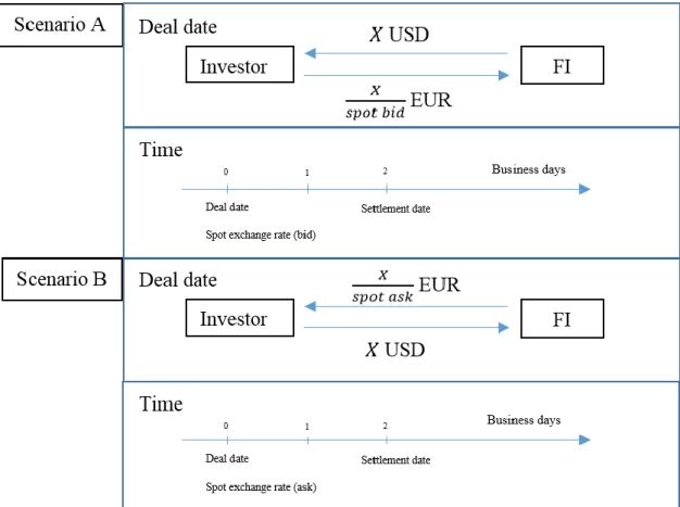
The two-sided nature of this contracts offers an intuitive insight to the cash-flows generated: they are the opposite from the perspective of either of the counterparties. Any cash a counterparty receives must have been paid by the other; no cash is lost. When an investor pays 100 000 Euros to receive 112 000 US Dollars from another investor at the ask-forward rate of 1.12 EUR/USD, the latter is receiving 100 000 Euros to pay 112 000 US Dollars at the ask-forward rate of 1.12 EUR/USD. If the former investor looks at the KID from the product he is about to invest in and sees that, according to the stress scenario, he may incur in an extreme loss of 40% of the initial investment, then the latter investor can conclude he may make an extreme profit of 40% of his initial investment.
30
The same reasoning applies to any other profit or loss generated by a milder event that does not qualify as extreme.
Intuitively, the following results must be verified:
• The potential profit/loss at the 10th, 50th and 90th percentiles relative to the
purchase of foreign currency shall correspond the potential profit/loss at
the 90th, 50th and 10th percentiles relative to the sale of foreign currency.
So, the unfavorable, moderate and favorable scenarios of the purchase will be symmetric to the favorable, moderate and unfavorable scenarios of the sale;
• The stress scenario of a sale, given by the VaR with a 99% of certainty,
must correspond to the symmetrical VaR of the purchase with a certainty of 1%.
Any deviations from the results stated above arise from the fact that the same price simulation will never produce the same result twice, no matter how close the results are between iterations.
Analytically, these results are only verified if the historical lognormal returns in the methodology are adapted to reflect what it means to have a return when investing in the FOREX market. The FX historical lognormal returns for a product in which the investor accepts to buy foreign currency in a future date are calculated as follows.
If one uses the historical exchange rate of a currency pair as the historical price of the PRIIP, when buying foreign currency, an investor obtains a positive return if, upon selling it, he earns more domestic currency than he originally paid to buy it. This happens when the foreign currency appreciates against the domestic currency and the indirectly quoted exchange rate falls; one will need less foreign currency to trade domestic currency than before. This means that the rise of an exchange rate translates in a negative return for the buyer of foreign currency and the return must be calculated as:
𝑟𝑖 = −𝑙𝑛 𝑆𝑖
𝑆𝑖−1 ( 15)
𝑟𝑖 – Return in period 𝑖;
31
Another way to check this result is to think about what one is paying and receiving when buying foreign currency. If one is acquiring US Dollars – foreign currency – then they have to pay Euros – domestic currency. The price to insert in the model is the Euros they have to pay. The exchange rate 𝑆 EUR/USD is quoted indirectly, so the price to pay
to receive 1 US Dollar is 1
𝑆 Euros. Assuming the exchange rate is quoted today at 𝑆𝑖−1
EUR/USD and tomorrow at 𝑆𝑖 EUR/USD, the price to pay today for 1 US Dollar will
be 1
𝑆𝑖−1 Euros and tomorrow will be
1
𝑆𝑖 Euros. According to the PRIIP methodology, the
lognormal return will be:
𝑟𝑖 = 𝑙𝑛 1 𝑆𝑖 1 𝑆𝑖−1 = 𝑙𝑛𝑆𝑖−1 𝑆𝑖 = 𝑙𝑛 𝑆𝑖−1− 𝑙𝑛 𝑆𝑖 = −(𝑙𝑛 𝑆𝑖 − 𝑙𝑛 𝑆𝑖−1) = − 𝑙𝑛 𝑆𝑖 𝑆𝑖−1 ( 8)
The computation of returns for the sale of foreign currency follows the opposite reasoning.
When selling foreign currency, an investor gets a positive return if, when buying it back he pays less domestic currency than he original received for selling it. This only happens when the foreign currency depreciates and the exchange rate rises; it will take more foreign currency to trade domestic currency. So, the rise of the exchange rate represents a positive return for the seller of foreign currency:
𝑟𝑖 = 𝑙𝑛 𝑆𝑖
𝑆𝑖−1 ( 9)
𝑟𝑖 – Return in period 𝑖;
𝑆𝑖, 𝑆𝑖−1 – Exchange rate in period 𝑖 and 𝑖 − 1.
Again, another practical way to check this result is as follows: If today someone
is selling US Dollar against Euros at an exchange rate of 𝑆𝑖−1EUR/USD and tomorrow
the rate moves to 𝑆𝑖 EUR/USD, they are paying US Dollars to receive Euros. The price
to pay today to receive 1 Euro is 𝑆𝑖−1 US Dollars and the price to pay tomorrow to receive
1 Euro is 𝑆𝑖 US Dollars, meaning the lognormal return shall be:
𝑟𝑖 = 𝑙𝑛 𝑆𝑖
𝑆𝑖−1 ( 10)
Until now, the exchange rate considered to compute lognormal returns has not been specified, only that it belongs to the currency pair one is interested in. Yet, since this report deals with price forecasts for FX forwards, the spot exchange rate may not be the
32
best variable to treat as a historical price; this leads to the additional treatment of the relevant historical series of forward exchange rates as the price of the FX forward.
As discussed in section 2.2.2, the forward exchange rate is calculated using the spot exchange rate weighted by the interest rate practiced in the countries that issue the
currencies traded16. Evaluating performance scenarios using historical time series of
forward rates based on the historical spot and relevant interest rates of the same period might be useful if the historical curve of forward rates behaves differently from the historical curve of spot rates, considering that the Regulation’s methodology only captures variations from any set of input prices. This result is discussed below in section 4.
A different way of interpreting the price data necessary to further advance with the PRIIP’s model application arises from the fact that, for each forward exchange rate a financial institution (FI) is willing to trade at, an investment may result in different possible outcomes for the investor; hence, the performance scenarios calculated may depend on the spot and forward exchange rates contracted at the deal date. This means that the implied interest rates, obtained from the ratio between the forward and spot rates, factor in the historical price of the FX forward, is the only variable capable of influencing the performance scenarios. So, an additional attempt is addressed in an effort to ensure accurate performance scenarios by applying the interest rates in force at the deal date to the historical time series of spot rates, thus obtaining forward rates determined from different spot rates but weighted constant interest rates.
Using spot exchange rates and, if deemed necessary, two sets of forward exchange rates weighted by variable and constant interest rates, of the past 6.1397 years – from
April 10th 2013 to May 29th 2019 – performance scenarios will be calculated for the
purchase and sale of 3 currency pairs17 with different contractual conditions – the forward
rate and deal date contracted – and an RHP of 12 months. The reason for calculating scenarios relating to the same FX products with different contractual conditions lies on the main objectives of this report, which are establishing a visual comparison to the same scale between scenarios obtained from this report’s interpretation of the model set out in
16 A forward rate must be computed using the spot rate and interest rates held for the same particular
day.
33
Regulation 2017/653 and scenarios obtained from a multiple number of FIs’ interpretations of the same Regulation’s rules, and drawing conclusions about the results. The first step towards the application of each methodology is gather KIDs from seven different FIs and extract the necessary information to, later on, use it in the analytical generation of the performance scenarios.
The following course of action shall be gather the historical time series18 of the
spot exchange rates for each of the three currency pairs and the annual interest rates for each of the four currencies that compose the three currency pairs used. For any approach involving interest rates, these will be extracted from Bloomberg’s database.
For the same date, spot and both forward rates’ series will be compared to infer the necessity of calculating performance scenarios for each type of exchange rate.
After assembling the necessary historical time series of exchange rates, both Regulation and ESAs’ methodologies will be applied and performance scenarios will be determined.
Finally, the obtained results will be confronted with the ones from third party FIs.
34
4. Results
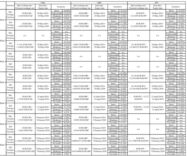
Table 1 in appendix D shows the performance scenarios of several banks claiming to follow the methodology laid out in the Regulations regarding PRIIPs and already allows for a preliminary conclusion about the different interpretations one can make of the Regulation’s rules.
It’s possible to observe the discrepancy between bank 1 and bank 2’s performance scenarios; despite them being determined for the same product with the same deal date and RHP, the slight difference of exchange rates do not justify any of the scenarios’ disparities.
The results for banks 2 and 4 point to an overall convergence in how both FIs interpret the model presented by the Regulation 2017/653 given the scenarios are alike for the same deal date, despite the exchange rates being moderately different. The fact that different spot and forward rates originate visually comparable scenarios for the same deal date supports the evidence that the forward exchange rate contracted by a FI must not affect the historical price of FX forwards and, thus, the performance scenarios.
Bank 3, despite presenting scenarios for a deal date 9 trading days prior to banks 1, 2 and 4, shares 99.3% of same historical sample of prices as the other 3 banks, i.e.,
while banks 1, 2 and 4 calculate scenarios using historical rates from May 27th 2014 until
May 28th 2019, bank 3 does so using historical rates from May 14th 2014 until May 15th
2019. This 9-day difference in historical data is, seemingly, enough for there to exist such significant deviations in the scenarios.
The same observation can be verified in banks 6 and 7’s scenarios. The deal dates in both banks differ in 1 month; while bank 6’s scenarios capture variations of prices
between January 6th 2014 and January 7th 2019, bank 7’s scenarios capture prices
variations from February 5th 2014 to February 6th 2019. The data indicates a 23-day
difference amongst a 1 280-day time series is sufficient to cause notable deviations. In the interest of comparing spot with forward exchange rates, the following step is converting spot in forward rates using interest rates. The 7 FIs offered FX forwards for
different currency pairs with the following deal dates: May 29th 2019, May 16th 2019,
April 12th 2018, January 8th 2019 and February 7th 2019. Generally, in order to compute
35
daily prices prior to the deal date. So, for instance, regarding the EUR/USD FX forward
with a deal date in May 29th 2019, one must, in the first approach, take the series of 1 280
spot exchange rates from May 27th 2014 to May 28th 2019 and the interest rates series
from EUR and USD of the homologous period19 and convert the nth spot rate in the nth
forward rate using the nth interest rates of each currency (𝑛 = 1, … , 1 280); in the second
approach, the nth forward exchange rate in the series is calculated utilizing the nth spot
exchange rate and the 1 280th interest rates of each currency20. The same reasoning is
made for the currency pairs and deal dates for which the FIs from table I calculate performance scenarios, resulting in 3 comparable time-series, as plotted in Appendix F.
Each graph from Appendix F demonstrates a similar curve behavior in any of the 3 exchange rates’ time-series. They indicate that, for a given time interval, whether one uses spot or the respective forward exchange rates in the methodology to calculate performance scenarios, their lognormal returns will be alike. In fact, the first approach, supported by the interest rate parity theory, eliminates any arbitrage opportunities created by a divergence in interest rates, meaning that an investor shall expect the same return from trading currencies at different times as from borrowing and depositing currencies at their respective interest rates and converting the foreign amount in domestic currency using the respective spot rate, which is to say lognormal returns from the spot and forward rates must remain roughly equivalent. The second approach consists of adjusting spot exchange rates with a constant factor (constant interest rates from the day before the deal date), which will only rescale the spot exchange rates and, thus, keep the lognormal returns unchanged.
Therefore, based on the premise that section 3’s methodology only captures prices’ variations for performance scenarios’ computations, these will be virtually identical whether one adopts spot or forward exchange rates as historical prices.
This report handles spot exchange rates for the performance scenarios’ assessment and the results are compiled in Appendix G’s tables V and VI. It is notable that for each FX forward, the set of 4 performance scenarios issues from a simulation of 20 000 future performances.
19 Rates extracted from Bloomberg’s database. 20 See Appendix E for calculations
36
In detail, the ESAs’ methodology reflects an attempt from the Joint Committee to enlighten FIs that performance scenarios may not follow a normal distribution.
Results from the Regulation’s methodology in table V suggest that unfavorable,
moderate and favorable scenarios – prices at the 10th, 50th and 90th percentiles,
respectively – are prices extracted from a normal distribution of future performances. For any of the 24 sets of assessed performance scenarios, the 20 000 prices generated follow
a normal distribution with a mean almost identical to the value of the product in the 50th
percentile; furthermore, the probability of a price being smaller or equal than the unfavorable scenario is roughly equal to the probability of a price being greater or equal than the favorable scenario.
Relating to results from the ESA’s Joint Committee’s interpretation of the Regulation’s methodology in table VI, each set of 20 000 simulations follow overall asymmetrical distributions, proposing that scenarios shall reflect the susceptibility of products to periods of high and low volatility.
37
5. Conclusion
The dissimilarity in observed results when comparing performance scenarios from third-party FIs, from this report’s interpretation of the Regulation’s methodology presented in section 3.1 and from the ESAs’ interpretation of the Regulation’s methodology presented in section 3.2 hints at how the Regulation 2017/653’s rules for the calculation of performance scenarios are susceptible of distinct interpretations by different FIs.
It’s important to note that the purpose of both Regulations arises from the need to inform non-professional investors about financial products’ risks and costs. From the point of view of these non-professional investors, their task of comparing similar products from different banks will not be easy due the existence of such misinformation generated by the banks’ diverging understanding of the methodology. The way the methodology is currently designed leads to a lack of understanding between different banks to provide investors with the most accurate information regarding financial products.
Also, ever since the Regulation 2017/653 came into effect in early 2018, it requires 5 years of historical prices for performance scenarios’ assessment. This constitutes a major drawback in the sense that FX market volatility has been at its lowest since 2014 as an effort from the European Central Bank (ECB) to stimulate economic growth and depreciate the Euro by decreasing interest rates. Low volatility coupled with high returns generates over-optimistic projections under the KID’s prescribed methodology.
In fact, an ESAs’ report concerning a revision on PRIIPs regulation dated back to February 8th 2019 states that the PRIIPs Delegated Regulation 2017/653 will be the target of an examination and review during 2019 to evaluate the necessity of changing RTSs regarding, for example, types of PRIIPs, costs and, the most important of all in the scope of this report, performance scenarios.
Hopefully, new RTSs concerning performance scenarios will lead to a convergent interpretation of the methodology, thus eliminating excessive fluctuations of results in KIDs amongst different FIs offering the same PRIIPs with equivalent contractual specifications, and encourage investors to make better informed decisions when faced with a wide range of PRIIPs.
38
6. References
EUR-Lex. (2014b), ―REGULATION (EU) No 1286/2014 OF THE EUROPEAN
PARLIAMENT AND OF THE COUNCIL. [ONLINE],‖
https://eur-lex.europa.eu/legal-content/EN/TXT/PDF/?uri=CELEX:32014R1286&from=EN. [Accessed 4 June 2019].
EUR-Lex. (2017), ―. COMMISSION DELEGATED REGULATION (EU)
2017/653. [ONLINE],‖
https://eur-lex.europa.eu/legal-content/EN/TXT/PDF/?uri=CELEX:32017R0653&from=EN. [Accessed 4 June 2019].
EUR-Lex. (2014a), ― DIRECTIVE 2014/65/EU OF THE EUROPEAN
PARLIAMENT AND OF THE COUNCIL. [ONLINE], ‖
https://eur-lex.europa.eu/legal-content/EN/TXT/PDF/?uri=CELEX:32014L0065&from=EN. [Accessed 4 June 2019]. Feenstra, Robert C., and Taylor, Alan M. (2008), International Macroeconomics, New York, NY: Worth Publishers
Financial Times. (2019), ― Peter Wells. [ONLINE],‖
https://www.ft.com/content/82409b6c-4a55-11e9-8b7f-d49067e0f50d. [Accessed 4 June 2019].
Hull, J.C. (2012), ― Value at Risk. Options, Futures and other Derivatives, (8th
ed.), Pearson
Joint Committee of the European Supervisory Authorities. (2018), ― PRIIPs –
Flow diagram for the risk and reward calculations in the PRIIPs KID. [ONLINE],‖
https://esas-joint-committee.europa.eu/Publications/Technical%20Standards/Flow%20diagrams%20for% 20the%20risk%20and%20reward%20calculations.pdf. [Accessed 4 June 2019].
Joint Committee of the European Supervisory Authorities. (2019), ―. Final
Report following joint consultation paper concerning amendments to the PRIIPs KID.
[ONLINE], ‖
https://eiopa.europa.eu/Publications/Reports/2019-02-08%20Final_Report_PRIIPs_KID_targeted_amendments%20%28JC%202019%206.2 %29.pdf. [Accessed 4 June 2019].
Sercu, Piet. (2008), International Finance: Putting Theory into Practice, (1st ed.),