UNIVERSIDADE FEDERAL DO CEARÁ CENTRO DE CIÊNCIAS
PROGRAMA DE PÓS-GRADUAÇÃO EM CIÊNCIA DA COMPUTAÇÃO MESTRADO ACADÊMICO EM CIÊNCIA COMPUTAÇÃO
JULIO ALBERTO SIBAJA RETTES
ROBUST ALGORITHMS FOR LINEAR REGRESSION AND LOCALLY LINEAR EMBEDDING
ROBUST ALGORITHMS FOR LINEAR REGRESSION AND LOCALLY LINEAR EMBEDDING
Dissertação apresentada ao Curso de Mestrado Acadêmico em Ciência Computação do Programa de Pós-Graduação em Ciência da Computação do Centro de Ciências da Universi-dade Federal do Ceará, como requisito parcial à obtenção do título de mestre em Ciência da Computação. Área de Concentração: Ciência da Computação
Orientador: Prof. Dr. João Fernando Lima Alcantara
Co-Orientador: Prof. Dr. Francesco Corona
Dados Internacionais de Catalogação na Publicação Universidade Federal do Ceará
Biblioteca Universitária
Gerada automaticamente pelo módulo Catalog, mediante os dados fornecidos pelo(a) autor(a)
R345a Rettes, Julio Alberto Sibaja.
Algoritmos robustos para regressão linear e locally linear embedding / Julio Alberto Sibaja Rettes. – 2017.
105 f. : il. color.
Dissertação (mestrado) – Universidade Federal do Ceará, Centro de Ciências, Programa de Pós-Graduação em Ciência da Computação, Fortaleza, 2017.
Orientação: Prof. Dr. João Fernando Lima Alcântara. Coorientação: Prof. Dr. Francesco Corona.
1. Outliers. 2. Estatística robusta. 3. Regressão linear. 4. Redução da dimensionalidade. 5. Locally Linear Embedding. I. Título.
ROBUST ALGORITHMS FOR LINEAR REGRESSION AND LOCALLY LINEAR EMBEDDING
Dissertação apresentada ao Curso de Mestrado Acadêmico em Ciência Computação do Programa de Pós-Graduação em Ciência da Computação do Centro de Ciências da Universi-dade Federal do Ceará, como requisito parcial à obtenção do título de mestre em Ciência da Computação. Área de Concentração: Ciência da Computação
Aprovada em:
BANCA EXAMINADORA
Prof. Dr. João Fernando Lima Alcantara (Orientador)
Universidade Federal do Ceará (UFC)
Prof. Dr. Francesco Corona (Co-Orientador) Universidade Federal do Ceará (UFC)
Prof. Dr. João Paulo Pordeus Gomes Universidade Federal do Ceará (UFC)
Prof. Dr. Amauri Holanda de Souza Júnior Instituto Federal de Educação, Ciência e Tecnologia
ACKNOWLEDGEMENTS
Writing this thesis was made possible by the financial support of the National Counsel of Technological and Scientific Development (CNPq). I would like to express my gratitude to my adviser Dr. Francesco Corona for his dedication and guidance in the entire process. His help, motivation and availability to work were essential to me. I want to thank Prof. João Paulo Pordeus for introducing me to the robust statistics field. I would also like to thank Prof. Carlos Brito for his exciting and interesting teaching methods. I am grateful to Dra. Michela Mulas for allowing me to work in her office, for all the support and for all the coffees.
Nowadays a very large quantity of data is flowing around our digital society. There is a growing interest in converting this large amount of data into valuable and useful information. Machine learning plays an essential role in the transformation of data into knowledge. However, the probability of outliers inside the data is too high to marginalize the importance of robust algorithms. To understand that, various models of outliers are studied.
In this work, several robust estimators within the generalized linear model for regression frame-work are discussed and analyzed: namely, the M-Estimator, the S-Estimator, the MM-Estimator, the RANSAC and the Theil-Sen estimator. This choice is motivated by the necessity of exam-ining algorithms with different working principles. In particular, the M-, S-, MM-Estimator are based on a modification of the least squares criterion, whereas the RANSAC is based on finding the smallest subset of points that guarantees a predefined model accuracy. The Theil Sen, on the other hand, uses the median of least square models to estimate. The performance of the estimators under a wide range of experimental conditions is compared and analyzed.
In addition to the linear regression problem, the dimensionality reduction problem is considered. More specifically, the locally linear embedding, the principal component analysis and some robust approaches of them are treated. Motivated by giving some robustness to the LLE algorithm, the RALLE algorithm is proposed. Its main idea is to use different sizes of neighborhoods to construct the weights of the points; to achieve this, the RAPCA is executed in each set of neighbors and the risky points are discarded from the corresponding neighborhood. The performance of the LLE, the RLLE and the RALLE over some datasets is evaluated.
RESUMO
Na atualidade um grande volume de dados é produzido na nossa sociedade digital. Existe um crescente interesse em converter esses dados em informação útil e o aprendizado de máquinas tem um papel central nessa transformação de dados em conhecimento. Por outro lado, a probabilidade dos dados conterem outliers é muito alta para ignorar a importância dos algoritmos robustos. Para se familiarizar com isso, são estudados vários modelos de outliers.
Neste trabalho, discutimos e analisamos vários estimadores robustos dentro do contexto dos modelos de regressão linear generalizados: são eles o M-Estimator, o S-Estimator, o MM-Estimator, o RANSAC e o Theil-Senestimator. A escolha dos estimadores é motivada pelo principio de explorar algoritmos com distintos conceitos de funcionamento. Em particular os estimadores M, S e MM são baseados na modificação do critério de minimização dos mínimos quadrados, enquanto que o RANSAC se fundamenta em achar o menor subconjunto que permita garantir uma acurácia predefinida ao modelo. Por outro lado o Theil-Sen usa a mediana de modelos obtidos usando mínimos quadradosno processo de estimação. O desempenho dos estimadores em uma ampla gama de condições experimentais é comparado e analisado.
Além do problema de regressão linear, considera-se o problema de redução da dimensionalidade. Especificamente, são tratados o Locally Linear Embedding, o Principal ComponentAnalysis e outras abordagens robustas destes. É proposto um método denominado RALLE com a motivação de prover de robustez ao algoritmo de LLE. A ideia principal é usar vizinhanças de tamanhos variáveis para construir os pesos dos pontos; para fazer isto possível, o RAPCA é executado em cada grupo de vizinhos e os pontos sob risco são descartados da vizinhança correspondente. É feita uma avaliação do desempenho do LLE, do RLLE e do RALLE sobre algumas bases de dados.
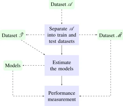
Figure 1 – Process of a single linear regression experiment . . . 63 Figure 2 – Performance of the algorithms by type of Outliers over Dataset 2; each
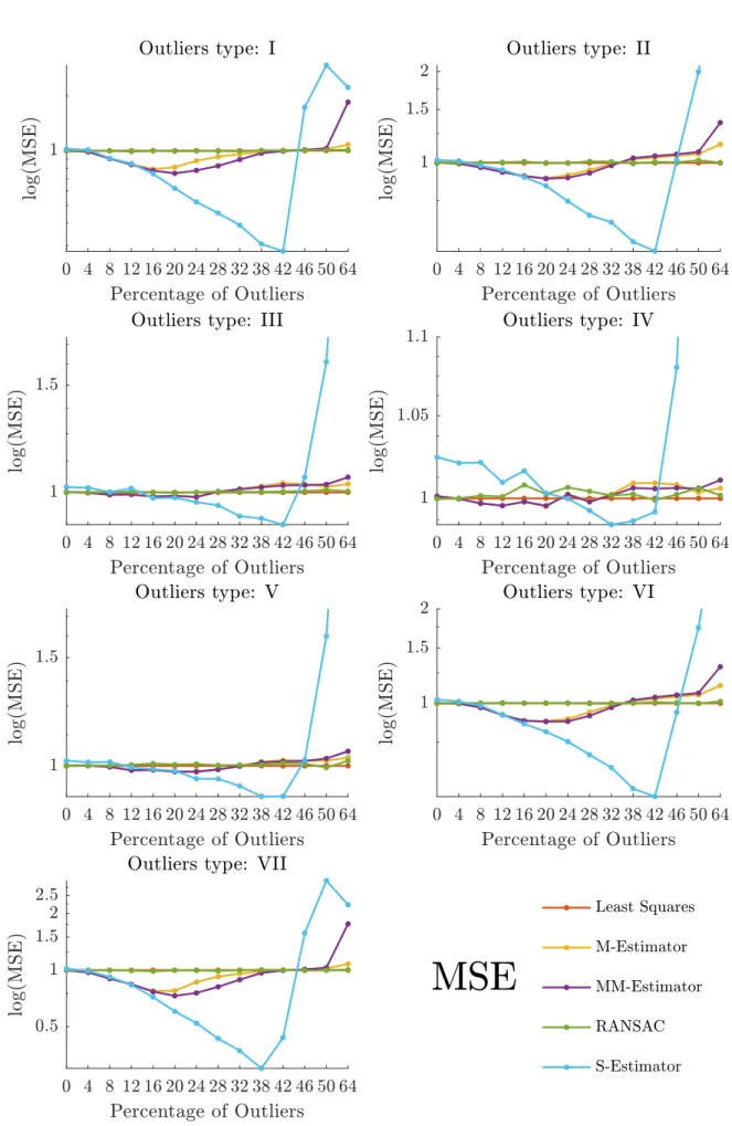
graphic shows the MSE in semilogarithmic scale (Normalized by the MSE of LS) of the estimations when varying the percentage of outliers. . . 69 Figure 3 – Performance of the algorithms by type of Outliers over Dataset 2; aach
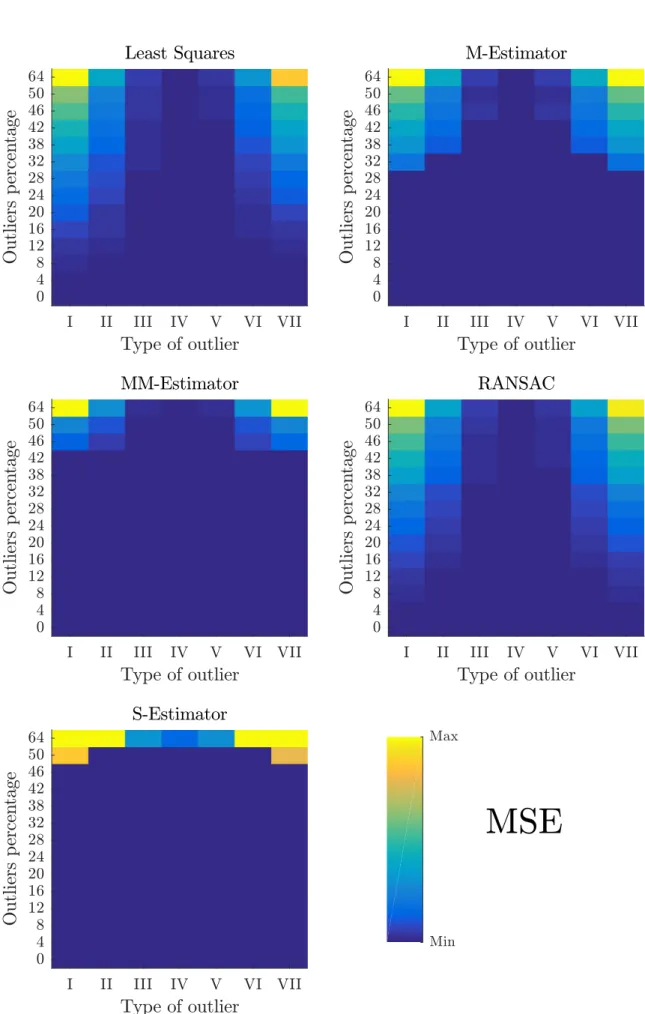
graphic contains the MSE of the estimations by each percentage of outliers. 70 Figure 4 – Performance of each algorithm over Dataset 2; each graphic contains the
MSE of one algorithm when varying type and percentage of outliers. . . 71 Figure 5 – Performance of the algorithms by percentage of Outliers over Dataset 2; each
one of them contains the MSE of the estimations made by all the algorithms over each type of outliers. . . 72 Figure 6 – Performance of the algorithms by type of Outliers over Dataset 3; each
graphic shows the MSE in semilogarithmic scale (Normalized by the MSE of LS) of the estimations when varying the percentage of outliers. . . 74 Figure 7 – Performance of the algorithms by type of Outliers over Dataset 3; each
graphic contains the MSE of the estimations by each percentage of outliers. 75 Figure 8 – Performance of each algorithm over Dataset 3; each graphic contains the
MSE of one algorithm when varying type and percentage of outliers. . . 76 Figure 9 – Performance of the algorithms by percentage of Outliers over Dataset 3; each
one of them contains the MSE of the estimations made by all the algorithms over each type of outliers. . . 77 Figure 10 – Performance of the algorithms by type of Outliers over Dataset 10; each
graphic shows the MSE in semilogarithmic scale (Normalized by the MSE of LS) of the estimations when varying the percentage of outliers. . . 79 Figure 11 – Performance of the algorithms by type of Outliers over Dataset 10; each
graphic contains the MSE of the estimations by each percentage of outliers. 80 Figure 12 – Performance of each algorithm over Dataset 10; each graphic contains the
MSE of one algorithm when varying type and percentage of outliers. . . 81 Figure 13 – Performance of the algorithms by percentage of Outliers over Dataset 10; each
Figure 14 – Performance of the algorithms byσ of the GBF over the real dataset; each graphic shows the MSE in semilogarithmic scale of the estimations when varying the number of centroids. . . 84 Figure 15 – Performance of the algorithms by number of centroids over the real dataset;
each graphic shows the MSE in semilogarithmic scale of the estimations when varying standard deviation used on the GBF. . . 85 Figure 16 – Performance of the algorithms by percentage of Outliers over Dataset 10; each
one of them contains the MSE of the estimations made by all the algorithms over each type of outliers. . . 86 Figure 17 – Performance of the algorithms by standard deviation of the GBF over the
yatch dataset; each graphic contains the MSE of the estimations when varying the number of centroids. . . 89 Figure 18 – Performance of the algorithms by number of centroids of the GBF over the
yatch dataset; each graphic contains the MSE of the estimations when varying the standard deviation . . . 90 Figure 19 – Performance of each algorithm over the yatch dataset; each graphic contains
the MSE of one algorithm when varying the standard deviation and the quantity of centroids used in the GBF. . . 91 Figure 20 – Process of a single experiment . . . 92 Figure 21 – Figures of the generated datasets . . . 93 Figure 22 – Representation of the trustworthiness and continuity scores of the Helix
embeddings. Each graphic contains the score values of one algorithm when varying the tolerance and the number of neighbors. . . 95 Figure 23 – Best 1-Dimensional embeddings of the algorithms. The x-dimension shows
the indexes of all the points and the y-dimension shows its embedding values. The ideal embedding representation is the one in which the inliers form a straight diagonal line. . . 96 Figure 24 – Best 1-Dimensional embeddings of the algorithms over the dataset without
squared figure with three color clusters. . . 96 Figure 26 – Best 2-Dimensional embeddings of the algorithms over the dataset without
outliers. The ideal embedding is a squared figure with three color clusters. . 97 Figure 27 – Representation of the trustworthiness and continuity scores of the S-Curve
embeddings. Each graphic contains the score values of one algorithm when varying the tolerance and the number of neighbors. . . 97 Figure 28 – Best 2-Dimensional embeddings of the algorithms. The ideal embedding is a
rectangular figure with well-defined color clusters. . . 98 Figure 29 – Best 2-Dimensional embeddings of the algorithms over the datasets without
outliers. The ideal embedding is a rectangular figure with well-defined color clusters. . . 98 Figure 30 – Representation of the trustworthiness and continuity scores of the Swiss Roll
embeddings. Each graphic contains the score values of one algorithm when varying the tolerance and the number of neighbors. . . 99 Figure 31 – ALOI’s Duck Dataset . . . 100 Figure 32 – Best Duck Embeddings of the algorithms. . . 100 Figure 33 – Duck Trustworthyness and Continuity. It contains the maximum TC scores
LIST OF TABLES
Table 2 – Popular functions for M-Estimators . . . 38 Table 3 – (ROUSSEEUW; YOHAI, 1984, p. 268) BDP and AE of an S-Estimator . . . 41 Table 4 – Types of outliers: defines the percentage of outliers that was taken from the
minandmaxcomponents . . . 64
Table 5 – Parameters used in the execution of the estimator . . . 66 Table 6 – Parameters of the Noise/Outliers creation . . . 67 Table 7 – Best MSE achieved by the algorithms in the 4B dataset. It contains the
configuration values in where the algorithms performs best. . . 83 Table 8 – Methodology and parameters of the dimensionality reduction experiments . . 93 Table 9 – Parameters used to generate the synthetic datasets . . . 94 Table 10 – It includes the best (max) TC score, the mean TC score and the lowest (min)
TC score obtained by the three algorithms over the three figures . . . 94 Table 11 – It contains the values of the parameters that correspond with the best scores of
AE Asymptotic Efficiency BDP Breakdown Point CR Croux and Ruiz-Gazen
IRLS Iteratively Reweighted Least Squares LLE Locally Linear Embedding
LMS Least Mean Squares LTS Least Trimmed Squares MAD Median Absolute Deviation ML Machine Learning
MSE Mean Squared Error MSS Minimal Sample Set OLS Ordinary Least Squares
PCA Principal Component Analysis RBF Radial Basis Functions
LIST OF SYMBOLS
x Scalars are denoted by lower case Roman letters
x Vetors are denoted by a lower case bold Roman letters
xj Denotes the jthscalar element in the vectorx
MT The transpose of a Matrix is denoted by superscript T M Matrix are denoted by uppercase letters
xj Denotes the jthvector of some matrixM
(w1, ....,wM) This notations represent a row vector withMelements
Rn×m Denotes the vector space of matrices with entries in the real numbers that have annbymrank
[a,b] Represents aclosedinterval fromatob
(a,b) Denotes theopeninterval excludingaandb
f(x) Function f evaluating a variablex
Ex[f(x)] Expectation of a functionf(x)with respect to a random variablex
P(x) ProbabilityPof a random variablex
| · | Absolut value or cardinality of a set
k · k Euclidean Norm of a vector
1 INTRODUCTION . . . 16
1.1 Machine Learning . . . 16
1.1.1 Unsupervised Learning . . . 17
1.1.1.1 Cluster Analysis . . . 18
1.1.1.2 Dimensionality Reduction . . . 18
1.1.2 Supervised Learning . . . 19
1.1.2.1 Classification. . . 19
1.1.2.2 Regression . . . 20
1.2 Outliers . . . 20
1.2.1 Models of Outliers . . . 21
1.2.2 Leverage Points . . . 24
1.3 Robustness . . . 24
1.4 Motivation and Objectives . . . 25
1.5 Overview and Organization of the Thesis. . . 26
I
ROBUST GENERALIZED LINEAR REGRESSION
28
2 ROBUST GENERALIZED LINEAR REGRESSION . . . 292.1 Generalized Linear Models . . . 29
2.1.1 Basis Functions . . . 30
2.1.2 Classic Least Squares . . . 30
2.1.3 Mean Squared Error . . . 31
2.1.4 Robustness Features in Linear Regression . . . 32
2.1.4.1 Equivariance . . . 32
2.1.4.2 Breakdown Point of an estimator . . . 32
2.1.4.3 Asymptotic Efficiency . . . 33
2.2 M Estimator. . . 34
2.2.1 Standard Deviation - Scale Estimate . . . 36
2.2.2 Functionρ . . . 37
2.2.3 Iterative Reweighted Least Squares. . . 37
2.3.1 Efficiency . . . 41
2.4 MM Estimator . . . 42
2.5 RANSAC . . . 43
2.5.1 Parameters . . . 44
2.6 Theil-Sen . . . 45
II
ROBUST LOCALLY LINEAR EMBEDDING
47
3 ROBUST LOCALLY LINEAR EMBEDDING . . . 483.1 Locally Linear Embedding. . . 48
3.1.1 Formulation of the LLE. . . 49
3.2 Principal Component Analysis . . . 51
3.2.1 Formulations . . . 52
3.2.1.1 Maximum Variance . . . 52
3.2.1.2 Minimum Error . . . 53
3.2.2 Weighted PCA . . . 55
3.2.3 RAPCA . . . 56
3.2.4 T2 and Q statistics for PCA . . . 58
3.3 Robust Locally Linear Embedding . . . 59
3.3.1 RLLE . . . 59
3.3.2 RALLE. . . 60
3.4 Trustworthiness and Continuity Measures . . . 61
III
EXPERIMENTS AND RESULTS
62
4 EXPERIMENTS ROBUST LINEAR REGRESSION . . . 634.1 Methodology of the experiments. . . 63
4.1.1 Synthetic datasets . . . 64
4.1.2 Real dataset . . . 65
4.1.3 Configuration . . . 65
4.2 Synthetic Datasets . . . 66
4.2.1 Generation . . . 66
4.2.2 Results . . . 67
4.2.2.3 Dataset 10 . . . 78
4.2.2.4 Dataset 4B . . . 83
4.3 Real Dataset . . . 87
4.3.1 Description . . . 87
4.3.2 Results . . . 87
5 EXPERIMENTS ROBUST LOCALLY LINEAR EMBEDDING . . . . 92
5.1 Methodology of the experiments. . . 92
5.2 Synthetic Datasets . . . 93
5.2.1 Results . . . 94
5.2.1.1 Helix . . . 95
5.2.1.2 S-Curve . . . 96
5.2.1.3 Swiss Roll . . . 98
5.3 Real Dataset . . . 99
5.3.1 Description . . . 99
5.3.2 Results . . . 100
6 CONCLUSIONS . . . 102
6.1 Linear Regression Conclusions . . . 102
6.2 Locally Linear Embedding Conclusions . . . 103
16
1 INTRODUCTION
1.1 Machine Learning
The main purpose of the Machine Learning (ML) is the implementation of algorithms capable of learning from data. For Murphy (2012, p. 1) the concept of ML is related with a constant effort to make automated methods for analyzing data. There is no doubt about the interdisciplinarity of the machine learning field, including probability and statistics, information theory, artificial intelligence and others (MITCHELL, 1997, 2).
In the machine learning universe, the word train is highly related with the word learn. According to Bishop (2006, p. 2), if someone uses a process that takes a data set and train to get the parameters of an adaptive modelβ, then the person is using the machine learning approach. In the training phase the algorithm is learning from the data. The next phases will depend on the kind of the problem; one part of the problems that we treat in this work involve, in the last phase, the prediction of outcomes for new unknown data (see Chapter 2). Then generalization is our aim, and it happens when an ML algorithm is capable to recognize or categorize a new data which was not part of the data set used in the training phase (BISHOP, 2006, p. 2).
Preprocessing, such as dimensionality reduction, is a common technique executed in the data before any type of training; it will depend however on the nature of the problem, but more importantly, on the nature of the ML implementation algorithm (BISHOP, 2006, p. 2). Another relevant process is the design, which implies the completion of four steps (MITCHELL, 1997, p. 13): The first step is to determine the type of training experience (from whom or where will the algorithm learn?). The second step is to determine the objective function (What do you want to minimize?). The third step is to determine the representation of the model structure (i.e Linear, Polynomial, Neural Network). The last step is to determine the learning algorithm (How to minimize the objective function?).
There are parametric and non parametric processes in machine learning. The use of parameters makes the dependency on the data distribution assumptions stronger; Nevertheless, the computation of the model becomes faster. On the other hand, the non-parametric models are more flexible but computationally heavier (MURPHY, 2012, p. 16).
p(D|β˜)is used, in which the modelβ˜is chosen in regard to maximize the probability of the data D. Using the maximum likelihood approach, it is not reasonable to merely focus on the
performance of the model over the training set, because overfitting (failure to generalize) is a frequent problem. To select the model that generalizes better, the data can be partitioned in two parts and using the biggest part to train and the other part, called the test set, to evaluate the performance of the model. Another option is to use cross-validation, the technique which splits the data intonfolds, and then iterates usingSias test set andD)Si∀ias the training set (BISHOP, 2006, p. 32-33).
Basically, learning paradigms can be divided into two principal types: the unsu-pervised learning or descriptive learning and the suunsu-pervised learning or predictive learning (MURPHY, 2012, p. 2). We are talking about them in the Sections 1.1.1 and 1.1.2. The range of problems that can be treated with an unsupervised learning algorithm is wider than the range of problems which the supervised ML is capable to solve (MURPHY, 2012). The latter can be explained because of the inherent requirement of the supervised ML to train with labeled data. Some authors believe in the capacity to extract information coming out from the pure data itself, and also hold that the unsupervised ML is more related with the learning capacity of the animals (including the human species) than the supervised ML (MURPHY, 2012, p. 9-10). In contrast to this, the most widely used type is the supervised ML (MURPHY, 2012, 3).
There is a third type of machine learning called reinforcement learning that is related to learning based on the reward/punishment obtained for executing actions (MURPHY, 2012, 2). Therefore the objective of reinforcement learning is to learn which choices would maximize the absolute reward; its learning process typically uses a kind of trial/error technique (BISHOP, 2006, 3). Examples of problems using the reinforcement learning type are puzzle games, manufacturing problems and scheduling problems (MITCHELL, 1997, p. 367-368). The detailed treatment of reinforcement leaning lies beyond the scope of this work.
1.1.1 Unsupervised Learning
18
The model β of parameters is made in the form of p(xi|β). The intention is to infer the properties from the modelβwithout having the right properties to correct the training process (FRIEDMANet al., 2001, p. 486). Examples of this type of learning are clustering and
dimensionality reduction.
1.1.1.1 Cluster Analysis
The cluster analysis technique, also known as data segmentation, is one of the most popular unsupervised learning procedures. As its name suggest, it is related to finding, inside of the dataset, subgroups or segments called subsets or clusters (FRIEDMAN et al., 2001, p.
501). In this technique, the elements of the dataset are identified by a set of properties and it is expected to obtain clusters, where all the elements inside each cluster have similar properties (FRIEDMANet al., 2001, 502).
1.1.1.2 Dimensionality Reduction
Dimensionality reduction can be useful in some contexts as a data pre-processing stage, still in other cases as a necessary procedure. Dimensionality reduction is a technique concerned with the transformation of the dimensionality of the data. As its name suggests this transformation is made to obtain a new meaningful dataset with less dimensionality than the original set (MAATENet al., 2009, p. 1).Some examples of real world datasets that commonly
need a reduction of their dimensionality to be processed are digital photographies, speech signals and fMRI scans (MAATENet al., 2009, p. 1). The reduction of the dimensionality of data can
also be helpful to achieve lossy data compression, data visualization and exploratory analysis (BISHOP, 2006, p. 561)(ROWEIS; SAUL, 2000, p. 1).
1.1.2 Supervised Learning
In supervised learning the objective is to learn from labeled data. This means that if we havenobservations in the dataset, each elementxihas another element or labelti. In other words, the data consist of a set of input vectorsxialong with their corresponding output vector ti∀i(BISHOP, 2006, p. 3).
The input vectorxican represent almost anything, from simple integers to phrases or audios. In the same way, the output can express a wide range of information, but it has to be represented into a categorical (qualitative, discrete) variable or nominal (quantitative, continue) variable. These conditions in the specification of the output lead to the categorization of the problem in two types: a classification problem when the output is categorical and a regression problem when the output is nominal. Besides classification and regression a special type of problem remains, it happens when the output presents qualitative and quantitative values. Then you can use a combination of methods used in the two first types if it is possible. (FRIEDMAN
et al., 2001, p. 10).
There exists a third type of supervised learning problem. It occurs when the output is an ordered variable (such as cold, warm, hot), but it is not in the scope of this work to explain the details of this problem (For details of this type see Friedmanet al.(2001, p. 10)).
1.1.2.1 Classification
Classification supervised problem arises when the output is represented using quali-tative variables. The most common and practical option is to encode all the possible outputs or categories using a numeric form. If there are only two categories (called binary classification), the simplest way is to encode using ‘1’ to represent one category and ‘0’ to represent the other category. On the other hand if there arek>2 categories (called multiclass classification) a K binary variable scheme is normally used. In this scheme each output variable is represented in a vectort∈Rk, and all the values inside the vector are zero except theith position that represents
20
over the inputx(BISHOP, 2006, p. 180). Applying the Bayes theorem,
p(Ck|xi,D) =
p(xi,D|Ck)p(Ck)
p(xi,D) (1.1)
and using the maximum posterior to solve the classification problem, we say that the model represents the valuesyi, such
yi=max
k p(Ck|xi,D)∀i. (1.2)
1.1.2.2 Regression
Regression is a type of supervised learning problem where the output variables are continuous. The inputs are also called explanatory variables and the outputs are the response variables. Using the probabilistic approach, regression is very similar to classification, since the main idea is to find the model in which
yi=maxp(yi|xi,D)∀i. (1.3)
In this work the models are represented by linear functions. The use of linear functions for regression is one of the most representative approaches and carries advantages for studying purposes (BISHOP, 2006, 137).
1.2 Outliers
The definitions ofOutlierfound in the literature are usually different from each other
and there is no consensus about which of them is the most accurate. The word outlier literally means something that stands outside of somewhere. It is important to understand that the context of the problem that you are trying to solve makes one definition of outlier fit better than another.
Using a viewpoint more focused on the linear regression problems, Rousseeuw e Leroy (1987, p. 7) define Outlier as a point iwhere “(xi,ti)deviates from the linear relation followed by the majority of the data, taking into account both the explanatory variables and the response variable simultaneously”. A broader definition can be found where Susantiet al.
Anscombe (1960) mentioned the three main causes of variability in the data, that can arise in the occurrence of outliers. The first one is the measurement errors and are mostly related to instrument errors or the misuse of them. The second cause is the execution faults (e.g. changes in the system, mis-selection of some samples, design errors). Finally the third one is the intrinsic variability of the data. Generally, it is not an easy task to identify which of the last three causes is the origin of an outlier (BARNETT, 1978), and to then apply some method to deal with the spurious data.
One technique that can come to mind is to simply erase or remove the data which show similar patterns with some definition of outlier, but we cannot simply remove the data points from the dataset (HUBER; RONCHETTI, 2009, p. 4). The main reasons are:
1. It is not trivial to recognize the outliers (even more in multidimensional problems) in one step and then make the regression.
2. Even executing a process to clean the dataset of outliers, is common to make false rejections and false retentions. The resulting data set still cannot have normal distribution, and this can culminate in a more difficult problem. It is better to use robust methods than two-step (reject-regress) approaches.
3. In Hampbel experiments, the performance achieved by the best robust procedures looks to be higher than the best rejection procedures. In addition to that, the traditional rejection methods seem to suffer ‘masking’ when multiple outliers affect the data. (Studies made by Hampbel 1974,1985)
Some people may ask why they have to take care of the outliers, probably thinking that their dataset only has clear or right values. The occurrence of data with peculiarities or attributes far away from the bulk of data is almost present in each data set in thereal world.
Hampel (1973) joined the conclusions in a wide range of scientific works, and he stained that between “5-10% wrong values in a data set seem to be the rule rather than the exception”.
In the Chapters 2 and 3, some algorithms designed to overcome the problem of outliers without (detecting and) deleting them from the dataset are described.
1.2.1 Models of Outliers
22
dataset would have so included. In this section are showed some models that describe the presence of outliers in one dataset; some are general models that can be used in almost any problem and others are more specific for linear regression problems.
Barnett (1978, p. ag248) proposes a list of model alternatives. He definesHas the hypothesis which claims that the data have anFdistribution, so
H:xj∈F∀j.
One second hypothesisH˜ determine the real distribution of the data, and at the same time, it is the explanation for the outliers present in the dataset. The following list explains the five alternatives of howH˜ can be defined:
(B1) Deterministic Alternative
xiis already known as an outlier, so
˜
H:xj∈F∀(j6=i).
(B2) Inherent Alternative
Here we have another distribution for all the data
˜
H:xj∈G6≡F∀ j.
(B3) Mixture Alternative
In this case we use λ, where 0≤λ ≤1, to make a mix of theF distribution from the original hypotesisHand another different distribution. Hence
˜
H:xj∈(1−λ)F+λG∀j.
(B4) Slippage Alternative
This alternative is the most used,
˜
H:
xj∈F∀(j6=i),
xi∈G.
Additionally to that, Barnett (1978) saids that frequentlyF≡G, but, ifF∼(µ,σ2)⇒ G∼(µ+a,σ2)orG∼(µ,bσ2), where(a>0)and(b>1).
(B5) Exchangeable Alternative
value is equally likely to be(1,2, ...,n).”
˜
H:
xj∈F∀j
xi∈G,
p(i= j) =n−1∀j.
The following model is given by Horataet al.(2013). Suppose that we are working
with simple linear regression, and therefore we have a target (output) vectort. For each element of the tvector we have an associated elementxin the inputs; then either ˜tis the target vector contaminated with ’one-sided’ outliers or ˆtis the target vector contaminated with ’two-sided’ outliers and theovector is generated using normal distribution. Then we can define:
˜
tj=tj+|oj|, ∀j, (1.4)
ˆ
tj=tj+oj, ∀j. (1.5)
The standard deviation σ of the ovector is an aspect not mentioned in the paper of Horata et al. (2013). It is possible to apply this generation model to other kind of problems, simply
considering the contamination of other target vectors or variables. That is done in order to
generate outliers in any dimension of the data.
The last outlier model described in this work is proposed by Wanget al.(2010). The
explanation is made with the assumption of working with simple regression, but the same as in the last model, it can be applied in any dimension of any problem. Then we have a target vector tand the list of steps are:
1. Find out the maximum valuemaxand the minimum valueminoft, calculate it’s meanµ
and standard deviationσ too.
2. Calculate an upperMupper margin and lowerMlower margin defined by
Mupper=||max| −σ|, (1.6)
Mlower=||min| −σ|. (1.7)
3. Generatekrandom values, where:
I⊆([max,(max+Mupper)]∪[(min−Mlower),min]) (1.8)
and|I|=k (1.9)
24
intention of providing an "adjusted to problem" model of outliers. For example, Ratcliff (1993, p. 511) knows that the common distribution of the time data for some chemical reactions is the ex-Gaussian with some specific parameters µ,σ andτ; then for the outliers he generates data with different sets of values for the parametersµ,σ andτ.
1.2.2 Leverage Points
A simple definition of leverage point is given by Rousseeuw e Yohai (1984, p. 257); they describe it as “an outlying in somexi,i∈(1, ...,n)”. The type of effect that can be made by a leverage point differs from the effect produced by outliers inti(ROUSSEEUW; LEROY, 1987, p. 7). Generally the occurrence of leverage points can be explained if thexi∃i are not generated artificially; In other words, this happens mostly with data obtained from an observable real problem (ROUSSEEUW; ZOMEREN, 1990, p. 634).
Xin e Xiaogang (2009, p. 137) affirm that the points lying farenoughfrom the spatial
center of the other explanatory variables have leverage. This definition of leverage point does not include any relation with the response variable but rather with the explanatory. However, the relation between the two variables(xi,ti)is also important because that can define the type of the leverage points.
There are two types of leverage points. If the outlyingxidoes not suggest a break in linear regression pattern followed by the bulk of the data, then we can affirm that it is agood
leverage point; Otherwise it is abadleverage point and represents a regression outlier (STUART,
2011, p. 6).
This work does not have as a goal to deal with leverage points, nor in analyzing the effects of them in the experiments, as we see in the Chapter 4. All the regressors chosen, except the ordinary least squares, protect in some degree from the outlying of the response variables.
1.3 Robustness
YOHAI, 1984, p. 256).
The notion of robustness in algorithms “signifies insensitivity to small deviations from the assumptions” (HUBER; RONCHETTI, 2009, p. 2) but involves more important concepts which persuades us not to trust totally in the assumptions made (STUART, 2011, p. 2). Thus, the resistance cannot be achieved by merely ignoring the points detected as spurious, like some people may think (ROUSSEEUW; LEROY, 1987, p. 8).
In the book Robust Statistics of Huber e Ronchetti (2009), the authors define a
list with 3 principal features (efficiency, stability and breakdown) that a good robust statistical procedure should have. The first statement says that it must have a reasonably high efficiency, almost optimal; the second one is related to the repercussion of small deviations from the assumptions made, and stands to maintain low the asymptotic variance of the estimate; the last one emphasizes that if some big deviations appear from the assumptions made, it will not result in a catastrophe.
1.4 Motivation and Objectives
Many of the methods used in the classical statistic are known to be non robust. There are classic algorithms that are highly affected by deviations on the assumptions made over the structure of the data. Some of these methods are highly used until today for solving their related problems; they are also combined with other methods and that makes their scope larger. Nowadays, it is common to deal with big high-dimensional datasets; and it makes complicated to understand the underlying structure of the data and then make the correct assumptions to create the models.
There is a motivation to comprehend how the robust statistics works. The linear models, as Bishop says, have “nice analytical properties and are probably the best way to start if you want to understand more sophistical models” (BISHOP, 2006, 137). Hence, in this thesis, the linear regression experiments are designed to understand how some both classic and robust algorithms perform under wrong data modeling assumptions. To achieve that, some outlier generation methods and some robustness features in liner regression have to be explained. The objective is to analyze the performance of the ordinary least squares, the M-Estimator, the S-Estimator, the MM-Estimator, the RANSAC and the Theil-Sen Estimator under a wide range of experimental conditions.
26
solutions with global minimum. The locally linear embedding is one of them and its robust approaches are just a few. This leads to propose a new robust approach for the locally linear embedding method. To do that, a formal description of the Locally Linear Embedding (LLE), the RLLE, the RALLE, the Principal Component Analysis (PCA), the weighted PCA and the RAPCA is developed. The objective is to analyze the performance of the LLE, RLLE and RALLE under some experimental datasets.
The performance of the linear regressors is measured with the mean squared error. Meanwhile, the performance of the dimensionality reduction techniques is evaluated with the trustworthiness and continuity.
1.5 Overview and Organization of the Thesis
In the numerical datasets, the rows represent instances or elements and the columns are the attributes or variables. Spurious elements can be found in almost any dataset of the real word. The main algorithms proposed to deal with the linear regression problems and the dimensionality reduction problems are not developed to cope with these type of instances. Therefore, anyone can suggest the use of some process to analyze and find the anomalous elements inside the data; then erase these points from the dataset and continue with the typical procedure. This approach is sometimes employed, but as it was explained above, it can caries some additional problems and it can be also an inviable procedure to apply. It can be hard to perceive some underlying features within the data, but is even harder to understand them completely.
The robust statistics area has been developed since the middle of the last century (Tukey (1960)) and until today (DIAKONIKOLASet al., 2016) it is still developing techniques
to cope with deviations from the assumptions made. In the scope of the thesis, the robust algorithms are designed to achieve the already mentioned problems without the application of some pre-processing phase. The treatment that the robust algorithms do to the data differs between each of them; and the performance also varies depending on the conditions that the spurious elements are disposed into the dataset.
data and also it is developed an analysis and a comparative of the performances of the algorithms. The Chapter 2 begins with the definition of the generalized linear models and the use of basis functions. A set of robust features in linear regression used to analyze the estimators are explained. Besides that, the robust linear regression algorithms are detailed. These are the M-Estimator, the S-Estimator, the MM-Estimator, the RANSAC and the Theil Sen.
Chapter 3 treats dimensionality reduction topics. The locally linear embedding, the principal component analysis, the weighted principal component analysis, the RAPCA and the RLLE are explained. Additionally, a new robust approach for the locally linear embedding is formally presented; its name is RALLE.
Inside the Chapter 4, the entire experimentation process of the linear regression is described. The generation of the synthetic datasets and the description of the real-world data are detailed. The results of the experiments are analyzed and used to compare the algorithms. The Chapter 5 is similar to the previous one, except, that it is related to the locally linear embedding algorithms.
Part I
2 ROBUST GENERALIZED LINEAR REGRESSION
Knowing that every dataset commonly includes some percentage of outliers, the im-plementation of robust regression algorithms to make the models is probably the most reasonable decision. At the same time, this choice may be required if is known that the residuals are not normally distributed or have an unknown distribution (SUSANTIet al., 2014, p. 351).
The main goal of regression is to predict continuous targetyfrom an input vectorx,
in that case we call itsimpleregression. If the prediction regards a target vectorythe problem is
calledmultivariateregression. In this work, we are concerned with simple linear regression.
Robust estimators of regression are the ones not highly affected by the outliers in the dataset (ROUSSEEUW; LEROY, 1987, p. 8). Huber e Ronchetti (2009, p. 8) mention that one goal of using robust methods “is to safeguard against deviations from the assumptions, in particular against those that are near or below the limits of detectability”.
2.1 Generalized Linear Models
We have a set ofnobservationsX={x1, ...,xn}, where each observationxi∈RD is associated with a target valueti∈R. The Ddimensional vectorsxi are called as input or explanatory variables because they are used to explain output or response variablet=y(x,β) +ε,
in whichε is the zero mean Gaussian noise andβis themdimensional vectors of parameters
(XIN; XIAOGANG, 2009, p. 9).
The generalized linear regression modely(x,β)is given by
y(x,β) =β0+ m−1
∑
j=1βjφj(x), (2.1)
whereφj(x)are known as basis functions and represent some transformation of the inputx; the
m−1 value define the quantity of basis functions used in the problem (BISHOP, 2006). Classic linear regression is a particular case of this general model in which φ(x) =x. Whatever the choice of the basis functions, the generalized regression model is linear in the parametersβ. The parameterβ0, also known as thebias parameter, corresponds to the output when all the inputs
are 0. If we add to the basis functions theφ0(x) =1 term, then we can write the Equation 2.1 as
follows
y(x,β) = m−1
∑
j=030
2.1.1 Basis Functions
The basis functionsφj(x)can be non-linear, thus allowingy(x,β)to be nonlinear in the inputs, but maintaining the linearity in the transformed inputs and in the parameters β. Examples of basis functions are polynomials, splines, radial basis functions, wavelets, logarithmic transformations, and others (KOHNet al., 2001, p. 139) (BISHOP, 2006).In the
following we show some examples of basis functions.
The first example are Radial Basis Functions (RBF). Various types of RBFs are popular in neural networks, and in general they are characterized by the calculation of distances between the input vectors and some other point called center (FRIEDMANet al., 2001, p. 36).
A commonly used type of RBF is the Gaussian Kernel
φj(x) =exp −
kx−ujk 2s2j
!
, (2.3)
where the termujfrom j= (1, ...,m)represents the centers andsj determines the scale of the space (FRIEDMANet al., 2001, p. 139) (BISHOP, 2006, p. 36). The norm of the 2 vectors can
represent the Euclidean distance or some other measure of spatial distance.
Another common example of basis function is the sigmoid. This basis function is defined as
φj(x) =σ
−kx−ujk sj
, (2.4)
whereσ(a)represents the logistic sigmoid function σ(a) =1/(1+exp(−a)). Note that the sigmoid uses the termsujandsj in the same way as Gaussian Kernel does.
In the following, we assume that the set of observationsX∈Rn×mhave been already transformed by theφjfunctions,∀jand withφ0=1.
2.1.2 Classic Least Squares
The Least Squares algorithm is the standard method for estimating, from data, the parametersβin generalized linear regression. The most commonly used variant of this method is called Ordinary Least Squares (OLS) (SUSANTIet al., 2014).
method which obtains the modelβ˜that minimizes the sum of squared errorE(β),
E(β) = 1 2
n
∑
i=1(ti−βTxi)2. (2.5)
To obtain the modelβ˜which minimizes the sum of squares, we set the derivative
∇βE(β) = n
∑
i=1(ti−βTxi)xTi (2.6)
to 0, obtaining that
0= n
∑
i=1(tixTi)−β˜T( n
∑
i=1(xixTi) (2.7)
If we solve the Equation 2.7 forβ, then we have the normal equations for the least squares:˜
˜
β= (XTX)−1XTt (2.8)
We can use theX†Moore-Penrose pseudo-inverse ofX, in the Equation (2.8) which is defined as follows:
X†≡(XTX)−1XT (2.9)
Minimizing the sum of squares error is equivalent to the maximization of the likeli-hood under the assumption of Gaussian noise distribution ofr(BISHOP, 2006, p. 141).
The OLS, as a classical method, is one of the chosen regression algorithms in this work being evaluated and compared in the experiments made.
2.1.3 Mean Squared Error
The Mean Squared Error (MSE) of an estimator is a classic measure used to de-termine the performance of an estimate (XIN; XIAOGANG, 2009, p. 238). It is defined as:
MSE(βˆ) =E[(β−βˆ)2] =Var(βˆ) + (E[βˆ]−β)2. (2.10)
This is known as the Bias-Variance trade off (MURPHY, 2012, p. 202). That is why even though the least squares is the one that achieves the lowest variance (among all the unbiased estimators), it will not necessarily reach the minimum MSE (FRIEDMANet al., 2001, p. 52). The MSE can
be calculated for a test dataset as
MSE(βˆ) =1 n
n
∑
i=132
2.1.4 Robustness Features in Linear Regression
There are many robust methods to choose, and it can be a difficult task to determine which methods are better than others. Beyond the performance (in terms of error or outliers), there are other global measures to compare the methods. Thus we discuss in more detail what is Efficiency, Breakdown Point and Equivariance (STUART, 2011, p. 8).
2.1.4.1 Equivariance
Given an estimator S with S(X,t) = β, we can say that S is equivariant if it is
possible to define linear transformations over some of the problem data and the model preserve consistency (ROUSSEEUW; LEROY, 1987, p. 116) (KOENKER; JR, 1978, p. 39). In other words an estimator can be considered equivariant if it can treat a problem as invariant under certain linear transformations (DAVIESet al., 1993, p. 1861). The three types of equivariance
and their linear transformations are (STUART, 2011, p. 9):
• The estimator is regression (shift) equivariant if an “additional linear dependencet→ t+Xa” can be reflected inβ→β+a:
T({(xi,ti+xiv)}) =T({(xi,ti)}) +v, ∀i. (2.12)
• The estimator is scale equivariant if it guarantees independence over the scale of the
response variablet, so any transformationt→atis reflected inβ→aβ:
T({(xi,cti)}) =cT({(xi,ti)}), ∀i. (2.13)
• The estimator isaffine equivariantif guarantee independence over the transformations of
the explanatory variablesXor reparametrization of design, whenX→AXis reflected in β→A−1β:
T({(XTA,t)}) =A−1T({(XT,t)}). (2.14)
2.1.4.2 Breakdown Point of an estimator
(1971), but it fell into disuse because Dohono and Huber (1983) introduced the finite-sample version.
In the least squares, only one point(outlier) can totally spoil the obtained model. However, this is not the case with others regressors that can handle a considerable portion of outliers in the data (ROUSSEEUW; LEROY, 1987, p. 9).
Rousseeuw e Leroy (1987, p. 10) describes the BDP as follows: If you have a dataset
(X,t)∈Rnxm and take a sampleZ whereZ ={(xi,ti)}p≤n
i=1, and the estimatorSthat produces the vector of parametersβ, whereS(Z) =β. Then if you corrupt a quantity of points j≤pof Z with arbitrary values, to obtain a new sampleZ′. Thus, the maximum effectE caused in the resultant model by the corruption ofZ is
E(j,S,Z) =sup||S(Z)−S(Z′)|| (2.15)
So we define the breakdown point ofT as
BDP(S,Z) =min(n
j:E(j,S,Z) =∞) (2.16)
BDP is a simple but helpful measure to evaluate the resistance of an estimator. The best proportion (or resistance) that can be achieved is 1/2 (HAMPEL, 1973, p. 97). The explanation for that maximum BDP can be done if you imagine the case when your data presents 50% of outliers; in that situation the regressor cannot be able to distinguish which part of your set is the right and which is the wrong (STUART, 2011, p. 9). Another relevant point to remark is that BDP is not the unique measure to evaluate robustness; as BDP, efficiency, equivariance and others as well are important to have a complete view of the resistance of the estimator.
2.1.4.3 Asymptotic Efficiency
Given an estimator S where S(X,t) =β, the efficiency e(S)is a ratio calculated by the minimum possible variance divided by the actual variance ofS. It is clear that the best
possible ratio is when the two variances in the division are the same (ratio equal to 1). In our context (regression), when the assumption of Gaussian distribution of the residualris satisfied,
the minimum possible variance is achieved by the least squares estimatorLSwithT(X,t) =β,˜ then the efficiency of a generalized linear regression estimatorSis (ANDERSEN, 2008, p. 9-10)
e(S) = E
(ti−β˜Txi)2
E[(ti−βTxi)2]
34
To close the definition, the phraseasymptotic efficiencyis used because the
calcula-tion of the efficiency is made over a sample with infinite size (STUART, 2011, p. 9).
2.2 M Estimator
Maximum Likelihood type estimators of M-Estimators was proposed by Huber(1973) with the intention of moderating the effect produced by the minimization of the squared error. The goal is to maintain the high efficiency of the OLS in the presence of normal error distribution and replace the objective function of the sum of squared residuals by some other robust function (ROUSSEEUW; LEROY, 1987, p. 148).
Using this type of estimators is possible to constrain the influence of values located ‘far away’ from the regression line (there the presence ofrealoutliers is probably higher). The
M-estimators employ some objective function that can decrease the influence in a smooth way, compared with the tough influence made by the distinction between the ‘good’ and the ‘bad’ observations of the classic rejection. Beyond that, it works better in the situations when the distribution is similar to normal but not normal (like a fatter distribution), because the rejection options are almost non-viable (HAMPEL, 1973, p. 10).
The M-Estimator principle is to find the modelβ˜which minimizes theE(β)function, defined as
E(β) = n
∑
i=1ρ(ri). (2.18)
The residualri=ti−βTxi, and the robustρ function is recommended to be symmetric and with a unique minimum at 0 (ROUSSEEUW; LEROY, 1987, p. 12). To choose the bestρ function is a must to know the distribution of the errors, but that is commonly unknown. Ifρ(ri) =r2i is used, the estimator is the same as OLS (STUART, 2011, p. 11-12). The original version of this algorithm is not scale equivariant, unless one change in the calculation of the functionρ be
made (HUBER; RONCHETTI, 2009, p. 106). The Equation 2.18 has to be converted into
E(β) = n
∑
i=1ρ
ri
s
, (2.19)
wheresis calculated with an implementation of some scale estimator of the standard deviation
The M-Estimators have good flexibility properties because of the possibility to choose the ρ function, plus they “generalize straightforwardly to multiparameter problems”
(HUBER; RONCHETTI, 2009, p. 45).
Now that the equivariant form of an M-Estimator was introduced, the process to calculate the parameters can be developed (STUART, 2011, p. 15-16). The first step is to derivate theβ˜with respect to themparameters and set this derivate equal to 0; before we introduce the ‘score function’ψ(u), which represents the first derivate of∇uρ(u), then we get
∇βE(β˜) = n
∑
i=1xi jψ
ri
s
=0∀j. (2.20)
Then the second definition is introduced, called ‘weight function’, which is defined by
wi=
ψ
ri
s ri s . (2.21)
Now if we made some substitutions in 2.20 we have:
n
∑
i=1xi jψ
ri
s = n
∑
i=1xi jψ
ri
s
ri
s
ri
s
=0∀j
n
∑
i=1xi jwi
ri
s = n
∑
i=1xi jwi(ti−β˜Txi) 1
s=0∀j
n
∑
i=1xi jwiβ˜Txi= n
∑
i=1xi jwiyi∀j
(2.22)
then we can represent 2.22 in vectorial form:
XTWXβ˜=XTWY
˜
β= (XTWX)−1XTWY.
(2.23)
WhereW∈Rn×nas the diagonal matrix with the values ofwi, or
W=diag(w) =
w1 ... 0
: . .. : 0 ... wn
36
This is not a closed form solution, because the value of the matrixWdepends in the valueβ˜and vice versa. Then can be applied the IRLS (see Section 2.2.3) to find ˜β. In the first step, the β is commonly calculated with the OLS, and then an iterative process is used, which is stopped after aqquantity of iterations or after achieving one tolerance valuee, wheree
represents the distance between the last two generated models.
The M-Estimators are better at generalizing if you compare with other robust esti-mators, because it is possible to constraint and shape the impact of the errors with the weight function (HUBER; RONCHETTI, 2009, p. 70). The implementation of redescending type of M-Estimators is recommended as well (see Section 2.2.2 for details). Huber e Ronchetti (2009, p. 70) are discordant. They belief that the use of redescending M-Estimators are overrated and they have to be employed with some precautions because the re-descending type can increase the minimax risk compensating no more than ‘a few percent of the asymptotic variance’ when extreme outliers are present. Consequently they suggest rejecting the most improbable data. (HUBER; RONCHETTI, 2009, p. 101).
2.2.1 Standard Deviation - Scale Estimate
In order to provide the model of the scale equivariance property, we have to im-plement some robust estimator of a scale (standard error), and include the resultant standard errorsinto the calculation of the objective function as we can see in the Equation 2.19.
(HAM-PEL, 1973). There are some types of Scale estimator, like pure scale, nuisance parameter and Studentizing.
In relation to the standard deviation of the M-Estimators the re-scaled Median Absolute Deviation (MAD) is one of the possible scale estimators to use.(HUBER; RONCHETTI, 2009, p. 106). The re-scaled MAD is
s=1.4826 MAD, (2.25)
where
MAD=Med{ti−βTxi∀i}=Med{ri∀i} (2.26)
2.2.2 Functionρ
In the case of the M-estimator (see Section 2.2), the S-Estimator (see Section 2.3) and the Weighted Principal Component Analysis (see Section 3.2.2), it is needed to select aρ
function that transforms the value of the residuals. There are some popular functions and, in this work we selected the Least Squares, the Huber (original propose), the Hampel and the Tukey bisquare (biweight) to compare their objective, score and weight functions, see table 2.
The redescending M-Estimators are one especial type of M-Estimators, because using some of them, it can be achieved the highest possible breakdown point in the M-Estimators (MÜLLER, 2004, p. 2). The redescending M-Estimators reduce the maximal asymptotic variance and it is indicated to use when the distribution can be long-tail or have extreme outliers (HUBER; RONCHETTI, 2009, p. 97).
One estimator is redescending if the score function or first derivative ψ of the objective functionρsatisfies lima→±∞ψ(u) =0. Specifically you can write it in the following way:
ψ(u) =0 for|u| ≥c, (2.27)
with anyc>0.
2.2.3 Iterative Reweighted Least Squares
The Iteratively Reweighted Least Squares (IRLS) uses the Newton-Raphson routine (FRIEDMANet al., 2001, p. 299). It is commonly employed if the applied basis functions have
any hidden parameter, or more generally, if is not possible to obtain a closed form from the derivative of the objective functionρ.
If σ is any function, for the OLS it is the squared residual σ(ri) =ri2, and ri =
ti−βTxiwhereβ ∈Rm. Then we want to minimize the function
E(β˜) = n
∑
i=1σ(ri). (2.28)
So the Newton-Rapshon takes the form:
β(c)=β(c−1)−H−1∇E(β), (2.29)
∇E(β) = n
∑
i=138 Table 2 – Popular functions for M-Estimators
Objective Function Score Function Weight Function
Cauchy c
2
2 log 1+ x c
!2
x
1+ x
c !2
1
1+ x
c !2 Hampel 1
2u2 if|u|<a a|u| −1
2a2 ifa≤ |u|<b
a
c|u| −1
2u2 c−b −
7a2
6 ifb≤ |u| ≤c a(b+c−a) if|u|>c
u if|u|<a asignu ifa≤ |u|<b
acsignu−u
c−b ifb≤ |u| ≤c 0 if|u|>c
1 if|u|<a a
|u| ifa≤ |u|<b
a c
|u|−1
c−b ifb≤ |u| ≤c 0 if|u|>c
Huber 1973 1
2u2 if|u|<a
a|u| −1
2a2 if|u| ≥a
(
u if|u|<a asignu if|u| ≥a
1 if|u|<a a
|u| if|u| ≥a
Least Squares
1
2u2 −∞≤u≤∞ u 1
L1 |u| signu 1
|u|
Tukey bisquare a2 6 1−
1− u
a !2
3
if|u| ≤a
1
6a2 if|u|>a
u
1− u
a !2
2
if|u| ≤a
0 if|u|>a
1− u
a !2
2
if|u| ≤a
and
H=∇∇E(β), (2.31)
wherecrepresents the number of the actual iteration. The process is stopped whencis equal to
aqquantity of iterations or after the distance between the last two generated modelsβ(c)and β(c−1) achieve one tolerance valuee. For the M-Estimators, fortunately the Equation 2.23 is
already in the format of a weighted least squares, then the calculation of
β(c)= (XTW(c−1)X)−1XTW(c−1)Y, (2.32) whereW(c−1) is determined applying the Equations 2.21 and 2.24 and using the vector of
40
2.3 S Estimator
The Robust Regression by means of S-Estimator is a linear regression algorithm proposed by Rousseeuw and Yohai (1984) with the main objective to minimize the residual scale (standard error) of the M-estimators (SUSANTIet al., 2014, p. 354). Its name comes from the
Scale-Estimator (ROUSSEEUW; YOHAI, 1984, p. 260). In order to introduce the S-estimator
the estimator of scales(r1, ...,rn)is presented, defined by the solution of
1
n
n
∑
i=1ρ
ri
s
=K, (2.33)
whereri=ti−βTxi,ri∈R ∀i,K is expected to beEΦ[ρ], Φthe standard normal andnthe number of elements of the dataset (ROUSSEEUW; YOHAI, 1984, p. 260). If there are multiple solutions to Equation 2.33, then choose sups; if there are no solution thens=0.
The chosen functionρ has to satisfy the following three conditions (STUART, 2011,
p. 24)(the first two are mandatory and the third one is to reach the 50% of BDP): 1. The functionρ is symmetric, continuously differentiable andρ(0) =0.
2. The function ρ is redescending, particularly exist some a>0 where ρ(a) is strictly increasing in the interval[o,a), and constant on the[a,∞).
3. EΦ[ρ]
ρ(a) = K ρ(a)=
1 2.
Then the S-estimator is used to obtain the model parametersβ, that minimize the˜ scale s, defined in the Equation 2.33, and is expressed by
˜
β=min
β s(r1(β), ...,rn(β)), (2.34)
and the scale estimator is
˜
σ =s(r1(β˜), ...,rn(β˜). (2.35)
to propose one estimator with a higher breakdown point than the M-Estimators, but at the same time share with them the “flexibility and nice asymptotic properties”.
If the selections of the function ρ, the constant K and the parameter aare made
properly, the 50% of BDP can be obtained, as demonstrated in the original proposal, when the authors (ROUSSEEUW; YOHAI, 1984, p. 261) use the Tukey Biweight (Bisquare) taking
a=1.547. Moreover in the same work, Rousseeuw e Yohai (1984, p. 262) generalize the calculation of the BPD for another combination of constant K and parametera(and keeping
tukey bisquare as theρ function), and then defining 0≤λ ≤ 1
2, they stand:
EΦ[ρ]
ρ(a) = K
ρ(a)=λ =⇒nlim→∞BDP=λ. (2.36) They also explain that if the value of a is increased it will yield to an estimator with better
asymptotic efficiency at Guassian Model, but as a consequence, the BDP will decrease.
The advantage of using the S-Estimator to estimate the modelβ˜over other estimators is the capacity to achieve the best BDP; also Least Mean Squares (LMS) and Least Trimmed Squares (LTS) can reach the 50% of BDP (ROUSSEEUW; LEROY, 1987, p. 144-145).
2.3.1 Efficiency
Asymptotic Efficiency (AE). “There is a trade-off between robustness and efficiency for M and S-scale estimators” (AELSTet al., 2013, p. 280). In the next table we show how the
S-estimators cannot estimate with a high BDP and at the same time with a high efficiency (under the error normal distribution assumption) (ROUSSEEUW; LEROY, 1987, p. 142).
Table 3 – (ROUSSEEUW; YOHAI, 1984, p. 268) BDP and AE of an S-Estimator
BDP AE a K
50% 28.7% 1.547 0.1995 45% 37.0% 1.756 0.2312 40% 46.2% 1.988 0.2634 35% 56.0% 2.251 0.2957 30% 66.1% 2.560 0.3278 25% 75.9% 2.937 0.3593 20% 84.7% 3.420 0.3899 15% 91.7% 4.096 0.4194 10% 96.6% 5.182 0.4475
BDP/effi-42
ciency, reaching the point of saying that the algorithm does not deserve to be called as “Robust” and it would be more appropriate to call it as just high BDP estimator (HUBER; RONCHETTI, 2009, p. 197). They also remark that the instability of the high breakdown point estimators is a known problem.
2.4 MM Estimator
This estimator was proposed by Yohai (1987) with the main intention of providing an estimator with 50% of BDP and at the same time with high asymptotic efficiency, under the assumption of normal distribution of the residuals. It is the first robust estimator proposed to have both high AS and BDP (STUART, 2011). The MM-estimator is a combination of one estimator with a high BDP (desirable 50%), an M-scale of the residuals and a computation of an M-Estimator.
The algorithm is defined in three steps:
1. Estimate the parameters ˆβ using a high BDP estimator, a 50% of breakdown point is recommended. Examples of 50% BDP estimators are S-Estimator, the Least Trimmed Squares and the Least Median Squares (see Rousseeuw e Leroy (1987) for details). 2. Use an S-Estimator with the parameters ˆβ, to calculate the scalesr (see Equation 2.35) of
the residuals. The objective function used in this step is calledρ0. The S-Estimator has to
be tuned (objective functionρ0and its parameters) to produce an estimate with 50% BDP.
3. This stage uses the M-estimator described in the Section 2.2 with small modifications. As equal to M-estimator a functionρ has to be chosen. Thisρ function has to be redescending (see Section 2.2.2) and satisfy that ρ(u)≤ρ0(u) ∀ u∈R. Then the goal of the
MM-estimator is to find the parameters ˜βwhich minimizes theE(β)function, defined as
E(β) = n
∑
i=1ρ
ti−β
Tx
i
sr
. (2.37)
It is opportune to note that in this stage the value of the scalesr will continues unchanged until the end of the algorithm. The score functionψ(u)represents∇uρ(u). Then to find the ˜βwe set∇βE(β˜) =0 which is
n
∑
i=1xi jψ
ri
sr
and must satisfyE(β˜)≤E(βˆ). From here the process is the same as that in the M-estimator algorithm, defining the same weight function (Equation 2.21).
Note that the first and the second stage can be joined as one stage if you implement an S-Estimator (tuned to be 50% BDP) to get the parameters ˆβand utilize the scale obtained in that process. In the S-Estimator stageρ0can be the Tukey Biweight function witha=1.547 to
provide to the S-estimator resistance to almost 50% of outliers (50% BDP). In the third stage, theρ of the M-Estimator can be again the Tukey Bisquare. The parametera=4.685 guarantees a 95% of asymptotic efficiency in the final estimator for the Tukey bisquare or the chosen of
a=2.697 guarantees a 70% of asymptotic efficiency (VERARDI; CROUX, 2009, p. 5).
2.5 RANSAC
The RANdom SAmple Consensus (RANSAC) algorithm proposed by Fischler e Bolles (1981) is an estimator developed by the computer vision community. In their work, they stand that the smooth treatment made in the M, SS, MM and other robust estimator by theρ
function is not always the best approach to deal with outliers (FISCHLER; BOLLES, 1981, p. 1).
If the dataset contains the input variablesX= [x1, ...,xn]Tand the output variables t∈Rn, RANSAC is an iterative parametric algorithm, also non-deterministic, that uses the minimal quantity of points needed to make themparameters of the modelβ. This quantity is
called the Minimal Sample Set (MSS). If the vector of the parametersβ∈Rm, then the MSS has to be equal to m. The thresholdδ is a parameter value of the algorithm and is required to calculate the consensus set(CS)S where
S =cs(β) ={xi:||ti−βTxi|| ≤δ, ∀i}. (2.39) The|S|represents the number of inliers and is a measure of how many points lie on the line described by β with a δ threshold. The distance between the line and a point is normally calculated with the Euclidean Norm. If a point xi⊂Sthen it is said thatxiis an inlier of the vector of parametersβ.
The RANSAC algorithm can be summarized in the following list of steps (HART-LEY; ZISSERMAN, 2004, p. 118):
44
2. Make the vector of parametersβusing some estimator and the sampleR, commonly the ordinary least squares is used.
3. Using the Equation 2.39, calculate the consensus set S and determine its number of inliners.
4. If the percentage of number of inliners |S|
n ≥τ reestimate the parameters of the model
but now using the sampleS to obtain the final vector of parameters ˜βand terminate. τ is a parameter of the algorithm, thus the value has to be previously defined.
5. If the percentage of number of inliners |S|
n <τ and the iterations made of this steps
are more thanN, select the consensus set obtained with the greatest quantity of inliners.
Otherwise, make another iteration starting from the step 1.
2.5.1 Parameters
To use the RANSAC algorithm, it has to be defined some parameters. This Section is about how to calculate the values of these parameters. The first approach described is given by the original paper by Fischler e Bolles (1981) and the parameters areδ,τ andN.
δ is a threshold which represents the tolerance of the residuals. The points that have
a distance closer thanδ from the model are called inliners. To obtain this threshold it is required
to calculate the standard errorσsbetween the modelβand the entire dataset. Then the original paper proposed to setσs≤δ ≤2σs (FISCHLER; BOLLES, 1981, p. 383).
τ is a percentage representing how many inliers you want to have in your consensus
set, and then to terminate the execution of the algorithm. A high value ofτ can be a good choice,
to assure that the modelβrepresents the bulk of the data and the points inside the consensus help to build a good ˜βas well. It is assumed that the probability of one point being in the consensus set of any wrong model isy. We expect than no more than half of the data to be outliers, so we
assume thaty<0.5. Then we have to make theyτn−MSS very low.
N represents the maximum number of iterations. pis commonly chosen to be 0.99
and represents the probability of taking a series of minimum sample setsM and that at least one of the sample sets be clean of outliers. Supposing that uis the probability to choose an inlier
selections to achieve(1−u|M|)N =1−p, doing manipulations
N= log(1−p)
log(1−u|M|) (2.40)
The second approach is more probabilistic (HARTLEY; ZISSERMAN, 2004, p. 118). The parameters are calculated, but it is needed two probabilities; the p has the same
interpretation made in the first approach. Forδp, let
δ = p(ti−βTxi≤δ)
= p
r
2
i
σs2≤ δ2
σs2
∀i,
(2.41)
and since ri
σs
is normal distributed, then δ
2
σs2has chi-square distribution. Then
δ =σs q
χk2,δ
p, (2.42)
wherekare the degrees of freedom (dimensionality of the data) andδpis a probability to get just inliers inside the thresholdδ. To calculate the quantity of iterations described in the Equation
2.40, the denominator of the fraction is recalculated, then
u|M|= m
∏
i=1 ˜n n≈
n˜
n
m
, (2.43)
where ˜nis the largest number of inliers found until that iteration.
2.6 Theil-Sen
Theil-Sen estimadors, was proposed by Theil (1950) and Sen (1968) and was origi-nally a simple linear regression estimator. The original Theil-Sen is as an estimator of slope, and it has a BDP of 29,3% and high asymptotic efficiency (ROUSSEEUW; LEROY, 1987, p. 67).
We define the input vectorx= [x1, ....,xn]T∈Rn; it represents some dataset coming fromnpoints, and a target vectort∈Rn. The original Theil-Sen defines the slope as
β1=Med
bi,j=
ti−tj
xi−xj
:xi6=xj,1≤i≤ j≤n
, (2.44)
where Med{ua:a∈A}is the median of the numbers in{ua:a∈A}. Then bias parameter is calculated as