www.earth-syst-dynam.net/3/139/2012/ doi:10.5194/esd-3-139-2012
© Author(s) 2012. CC Attribution 3.0 License.
Earth System
Dynamics
On the relationship between metrics to compare greenhouse gases –
the case of IGTP, GWP and SGTP
C. Azar and D. J. A. Johansson
Physical Resource Theory, Chalmers University of Technology, 41296 Gothenburg, Sweden Correspondence to:D. J. A. Johansson (daniel.johansson@chalmers.se)
Received: 18 January 2012 – Published in Earth Syst. Dynam. Discuss.: 6 February 2012 Revised: 19 September 2012 – Accepted: 8 October 2012 – Published: 2 November 2012
Abstract.Metrics for comparing greenhouse gases are ana-lyzed, with a particular focus on the integrated temperature change potential (IGTP) following a call from IPCC to in-vestigate this metric. It is shown that the global warming po-tential (GWP) and IGTP are asymptotically equal when the time horizon approaches infinity when standard assumptions about a constant background atmosphere are used. The dif-ference between IGTP and GWP is estimated for different greenhouse gases using an upwelling diffusion energy bal-ance model with different assumptions on the climate sensi-tivity and the parameterization governing the rate of ocean heat uptake. It is found that GWP and IGTP differ by some 10 % for CH4 (for a time horizon of less than 500 yr), and
that the relative difference between GWP and IGTP is less for gases with a longer atmospheric life time. Further, it is found that the relative difference between IGTP and GWP increases with increasing rates of ocean heat uptake and increasing cli-mate sensitivity since these changes increase the inertia of the climate system. Furthermore, it is shown that IGTP is equiv-alent to the sustained global temperature change potential (SGTP) under standard assumptions when estimating GWPs. We conclude that while it matters little for abatement policy whether IGTP, SGTP or GWP is used when making trade-offs, it is more important to decide whether society should use a metric based on time integrated effects such as GWP, a “snapshot metric” as GTP, or metrics where both economics and physical considerations are taken into account. Of equal importance is the question of how to choose the time hori-zon, regardless of the chosen metric. For both these overall questions, value judgments are needed.
1 Introduction
A range of metrics for comparing and aggregating the cli-mate effect of different greenhouse gases has been proposed. The most widely applied metric is the global warming po-tential (GWP). When estimating the GWP, the radiative forc-ing from a pulse emission, say 1 kg of gasX at timet= 0, is integrated until an arbitrary time horizonH, and divided by the result of an equivalent integration for the reference gas, usually CO2. GWP is the standard option when
compar-ing emissions of different greenhouse gases, e.g. in the Ky-oto prKy-otocol. It was originally developed by Rodhe (1990), Shine et al. (1990) and Lashof and Ahuja (1990). See Forster et al. (2007) for the estimates of GWP values developed for IPCC’s Fourth Assessment Report.
An alternative to the GWP that has received more attention recently is the global temperature change potential (GTP). When estimating the GTP the temperature response at time t=Hfrom a pulse emission of gasXat timet= 0 is divided by the equivalent temperature response for a reference gas, usually CO2. It should be noted that GTP only considers
the temperature response att=H. Thus, it is different from GWP in the sense that GWP is an integrative measure (of the radiative forcing contribution over the entire period). GTP was initially proposed by Shine et al. (2005).
following a pulse emission of a gasX compared to “the in-tegral of the temperature change” following a pulse emission of CO2.
Such a measure has been discussed previously by, for in-stance, Fisher et al. (1990), Rotmans and den Elzen (1992), Shine et al. (2005, p. 298), IPCC (2009), Gillet and Matthews (2010) and Peters et al. (2011). We here refer to this metric as theIntegrated Global Temperature change Po-tential (IGTP). Note that it is not GTP that is integrated, but the temperature response from gasX divided by the inte-grated temperature response from the reference gas.
In addition to GWP, GTP and IGTP, Shine et al. (2005) proposed aSustained Global Temperature change Potential (SGTP)as the temperature response at timet=H of a gas X emitted with a constant (sustained) rate (1 kg yr−1) di-vided by the temperature response at timet=H following sustained emissions of CO2(1 kg yr−1). Fisher et al. (1990)
also estimated halocarbon global warming potentials, i.e. a metric for the integrated warming effect of various halocar-bons compared to CFC 11, that was defined in the same way as SGTP with the main difference that infinite time horizons were used. They could use infinite time horizons since halo-carbons have exponential decay rates (which ensure conver-gence of the relevant integrals).
The purpose of our paper is to analyze the properties of IGTP and demonstrate its relationship with GWP and SGTP. Relations between IGTP, SGTP and GWP have been noted in the literature. O’Neill (2000) showed that IGTP and GWP are equivalent when the time horizon approaches infinity un-der special conditions. Shine et al. (2005) find a “near equiv-alence” between SGTP and GWP. This implies that IGTP and GWP are also near equivalent since IGTP and SGTP, as will be shown in this paper, are identical under “stan-dard” assumptions when calculating GWP values, i.e. con-stant radiative efficiencies (defined as the radiative forcing in W m−2kg−1) and constant atmospheric adjustment times for the gases compared. Sarofim (2012) analyzed SGTP val-ues for methane under the assumption of varying background concentrations. Further, Fisher et al. (1990) observe numer-ically that steady state values for SGTP (or HGWP in their terminology) are closely related to IGTP.
Recently, Peters et al. (2011) observed a close relationship between IGTP and GWP. In their paper, they conclude that “further modeling would be required to confirm these obser-vations”. In our paper, we use an upwelling diffusion energy balance model instead of the impulse response function ap-proach they take to estimate IGTP. In addition, we carry out a more systematic sensitivity analysis with respect to the cli-mate sensitivity and vertical heat diffusivity.
In Sect. 2, we present our model. The results are pre-sented in Sect. 3 which also contains our sensitivity analysis. In Sect. 4 we explain our results. Conclusions are given in Sect. 5. In the appendices, we formally show that IGTP and SGTP are equivalent measures (under standard assumptions about constant atmospheric adjustment times and constant
radiative efficiencies), and that IGTP and GWP are asymp-totically equal as the time horizon approaches infinity.
2 Method
In this section, we present the method used to calculate IGTP (and GWP). IGTP is defined as
IGTP(H )=
H
Z
0
TPx(t )dt
, H
Z
0
TP,CO2(t )dt (1)
where TPx(t ) is the temperature response at time t from a pulse emission of 1 kg of gas X at time 0 (and simi-larly for the temperature response for a pulse emission of 1 kg of CO2). In Appendix A we show that IGTP is
identi-cal to SGTP (under standard assumptions when identi-calculating GWPs). Thus all results presented in this paper that hold for the relationship between IGTP and GWP also hold for the relationship between SGTP and GWP (under the assumption of constant atmospheric adjustment times and constant radia-tive efficiencies).
Further, GWP is defined as
GWPx = H
R
0
CPx(t ) Fxdt H
R
0
CP,CO2(t ) FCO2dt
(2)
whereCPx(t )is the change in mass of greenhouse gasX in the atmosphere at timetfollowing a pulse emission (of 1 kg) at timet= 0, andFx is the radiative efficiency per kg of gas X in the atmosphere. We assume, as stated earlier, that the radiative efficiency and the atmospheric adjustment times are constant, which is standard when estimating GWP.
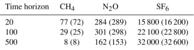
Table 1.IGTP estimates for CH4, N2O and SF6(with GWP values
in brackets).
Time horizon CH4 N2O SF6
20 77 (72) 284 (289) 15 800 (16 200) 100 29 (25) 301 (298) 22 100 (22 800) 500 8 (8) 162 (153) 32 000 (32 600)
In the standard set up, climate sensitivity is set to 3 K for a doubling of the atmospheric CO2concentration in line with
IPCC’s best estimate (Solomon et al., 2007). The likely range for the climate sensitivity is according to IPCC 2–4.5 K for a doubling of the atmospheric CO2 concentration. We use
this range in our sensitivity analysis. The ocean heat mixing in the UDEBM is determined by the vertical heat diffusivity and the upwelling rate. The upwelling rate is set to 4 m yr−1 (see Raper et al., 2001; Johansson, 2011; Meinshausen et al., 2011a) and the base case diffusivity is set to 2 cm2s−1. In order to emulate the ocean heat uptake and the surface tem-perature response in more complex models, a diffusivity in the range 0.5–5 is often used in UDEBMs (see Raper et al., 2001; Johansson, 2011; Meinshausen et al., 2011a; Baker and Roe, 2009; Olivi´e and Stuber, 2010). In the sensitivity analysis, we set this parameter at 0.5 and 4 cm2s−1 as al-ternatives to our base case assumption. In Appendix B, we demonstrate that our choice for these parameter values, in the base case as well as in the sensitivity analyses, is com-patible with the measured global average surface temperature change over the past hundred years.
For the atmospheric adjustment times for CH4, N2O, SF6
and CO2, we use the assumptions that are used when
esti-mated GWP in IPCC AR4, see Forster et al. (2007). The radiative efficiency measured per kg gas is also taken from Forster et al. (2007).
For forcings that are globally rather heterogenous (e.g. ozone, aerosols and contrails), an equal change in global mean radiative forcing gives a different global mean temper-ature response, i.e. the climate efficacies are not equal (see e.g. Hansen et al., 2005). It could be argued that under such conditions global warming potentials should be recalculated so that the climate efficacy of gasXis taken into account. In our calculations, we have assumed that the climate efficacies are equal to one throughout the paper.
3 Results: comparison of IGTP and GWP
We start by presenting numerical estimates for the GWP and IGTP for CH4, N2O and SF6in Table 1.
It can be noted that the GWP and IGTP values are close (see also Azar and Johansson, 2012 and Peters et al., 2011). One may also note that the 100 yr IGTP values for methane are slightly higher than its corresponding GWP val-ues, whereas the opposite holds for SF6. We will return to
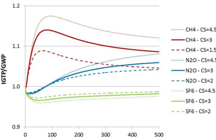
Fig. 1.IGTP/GWP ratio for CH4, N2O and SF6depending on the
time horizonH(in years).
this feature later on in the paper and see how it results from the fact that the gases have significantly shorter and longer perturbation life times than CO2.
The estimates for the IGTP/GWP ratios as a function of the time horizon,H, for CH4, N2O and SF6with CO2as the
reference gas, can be seen in Fig. 1. The difference between GWP and IGTP is typically around or less than 10 %. Sensitivity analysis
In this subsection, we focus on how the ratio between IGTP and GWP is affected by changes in the vertical heat diffusiv-ity and climate sensitivdiffusiv-ity.
An increase in the vertical heat diffusivity results in the temperature increasing more slowly in response to changes in the radiative forcing, see e.g. Hansen et al. (1985) and Jo-hansson (2011). This magnifies the difference between the equilibrium temperature change for a given forcing and the actual temperature change. As a consequence, the higher the heat diffusivity, the higher the inertia of the climate system, and the more IGTP will deviate in relative terms from GWP for all greenhouse gases (see Fig. 2). Decreasing the vertical heat diffusivity has the opposite effect, i.e. the IGTP/GWP ratio will for both short-lived and long-lived greenhouse be-come closer to unity.
Changing the climate sensitivity has a similar effect as changing the effective vertical heat diffusivity, since a larger climate sensitivity implies that the temperature responds, in relative terms, more slowly to changes in radiative forcing, see e.g. Hansen et al. (1985). This is shown for CH4, N2O
and SF6in Fig. 3. Decreasing the climate sensitivity has the
opposite effect, i.e. the IGTP/GWP ratio will for both short-lived and long-short-lived greenhouse become closer to unity.
Finally, in Appendix C, we present numerical values for IGTP for CH4, N2O and SF6for different assumptions on the
Fig. 2.IGTP/GWP ratio for CH4, N2O and SF6depending on
ef-fective vertical heat diffusivity.K, the vertical heat diffusivity, is given in cm2s−1.
horizon (from 20 to 500 yr) changes IGTP values by a fac-tor of two for SF6 and N2O, and almost a factor of 10 for
methane, but changes in the climate sensitivity and the heat uptake only affect the IGTP values by a few percent (in the absolute majority of cases).
4 Interpreting the relationship between GWP and IGTP
In this section we aim to explain and interpret the results pre-sented in Sect. 3. The ratio of IGTP and GWP is given by dividing Eq. (1) with Eq. (2), i.e.
IGTP(H ) GWP(H ) =
H
R
0
TPx(t )dt
H
R
0
TP,CO2(t )dt
,
H
R
0
CPx(t ) Fxdt H
R
0
CP,CO2(t ) FCO2dt . (3)
The equivalence between IGTP and GWP can be understood by rewriting the ratio IGTP/GWP in the following way
IGTP(H ) GWP(H ) =
H
R
0
TPx(t )dt H
R
0
λCPx(t ) FXdt H
R
0
λCP,CO2(t ) FCO2dt H
R
0
TP,CO2(t )dt
. (4)
Equation (4) was obtained by multiplying the expression in Eq. (3) byλ, the climate sensitivity, in both the numerator and the denominator. When multiplyingCPx(t ) Fx byλwe get the equilibrium temperature response for gasX. Thus, the first ratio on the right hand side of Eq. (4) is the grated (transient) temperature change divided by the inte-grated equilibrium temperature change for a gasX (follow-ing a pulse emissions).
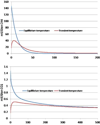
The equilibrium and the transient temperature responses of CH4 are illustrated in Fig. 4 (upper panel). As seen in
Fig. 3.IGTP/GWP ratio for CH4, N2O and SF6depending on
cli-mate sensitivity. CS, the clicli-mate sensitivity, is given in Kelvins per CO2equivalent doubling.
Fig. 4, the equilibrium temperature response is higher than the transient response for the first two decades due to heat uptake by the oceans, thereafter the transient temperature re-sponse is higher than the equilibrium rere-sponse due to heat release from the oceans. The integrated equilibrium temper-ature response (the area under the blue curve) is larger than the integrated transient temperature response (the area under the red curve) for any time horizonH, but the areas under the two curves approach the same value asymptotically asH approaches infinity.
This asymptotic behavior can be understood in physi-cal terms; the (integrated) radiative forcing must eventually manifest itself in (integrated) temperature change (see Ap-pendix D for a formal proof of this). Thus, the first ratio on the right hand side in Eq. (4) will be less than one and asymptotically approach one when the time horizonH ap-proaches infinity. Similar arguments hold for the second ra-tio, as will be discussed below, and for that reason the IGTP to GWP ratio becomes equal to unity as the time horizon approaches infinity, see Appendix D, O’Neill (2000), and Peters et al. (2011).
The second ratio on the right hand side of Eq. (4) is the integrated equilibrium temperature change divided by the in-tegrated temperature change for a pulse emission of CO2(see
lower panel, Fig. 4). Here the same arguments can be used as for CH4above, although the time scales involved when
ap-proaching unity is much longer because of the much longer perturbation life time of CO2. Hence, the second ratio on the
right hand side in Eq. (4) will be larger than one and asymp-totically approach one asHapproaches infinity.
The overall ratio in Eq. (4) will thus become slightly larger than one when CH4is gasX, since the ratio for CH4(the first
ratio on the right hand side) will reach unity faster than the ratio for CO2 since methane has a much shorter life time.
This explains the result shown in Fig. 1.
Fig. 4.Equilibrium and transient temperature response for a pulse emission of CH4(upper panel) and CO2(lower panel).
unity more slowly than the ratio for CO2. Thus the
IGTP-to-GWP ratio becomes less than one for SF6. Rotmans and den
Elzen (1992) also noted that the ratio IGTP-to-GWP is higher for gases with short life times, although they used slightly different concepts for IGTP and GWP.
For N2O the IGTP-to-GWP ratio is initially less than one,
but then becomes larger than one. This is explained by the fact that for short time horizons, an emissions pulse of N2O
decays from the atmosphere more slowly than CO2, but on
longer time horizons an emissions pulse of N2O decays more
rapidly than CO2.
The observation that the IGPT over GWP ratio is lower than one initially, then slightly higher than one, and then eventually returns asymptotically to one for N2O is in fact
a generic result. It also holds for CH4(which can be seen if
one looks carefully in Fig. 1 for the first few years1) and SF6
(which would be seen in Fig. 1 if the time horizon had been extended2), and more generically for all gases with constant decay rates in between those of CH4and SF6.
1Since CO
2(approximately) decays with a series of
exponen-tial time constants, one of which is much shorter than the decay time constant of methane (around 1.2 versus 12 yr according to the IPCC AR4 estimate), the IGTP-GWP ratio becomes less than unity the first few years.
2The ratio becomes higher than unity for time horizons so long
as most of SF6has decayed away (see also Peters et al., 2011). The
Explanation of the results in the sensitivity analysis
If there is no inertia in the climate system, it can be seen right away from Eq. (4) that the IGTP-to-GWP ratio will become equal to one (both ratios in the right hand side of Eq. (4) are equal to unity, since there is no difference between transient and equilibrium temperature response). Now, when consid-ering the inertia of the climate system (that results from the heat capacity of the oceans) the IGTP-to-GWP ratio will de-viate from unity. The larger the inertia is (as a result of higher climate sensitivity or higher diffusivity), the more the devia-tion of the ratio from unity will be. This is the fundamental reason behind the results of the sensitivity analysis presented in Figs. 2 and 3.
5 Conclusions
This paper addresses similarities between different metrics to compare greenhouse gases, in particular between GWP and IGTP. A near equivalence between IGTP and GWP is demonstrated. IGTP and GWP are near equivalent in two ways: (1) they are identical if there is no thermal inertia in the climate system; (2) they are asymptotically equal when the time horizon approaches infinity. The values differ by, at most, some 10 % in the cases studied here. Our research cor-roborates the results by Peters et al. (2011) and Rotmans and den Elzen (1992) who used different modeling approaches.
We also find a rather general relationship between IGTP and GWP. The ratio IGTP to GWP (for a time horizon in the range a decade to several centuries) is slightly higher than unity for gases with relatively short atmospheric life times (say methane), and lower than unity for gases with relatively long atmospheric life times (say SF6). However, if one
con-siders time horizons for the analysis that stretch from just a few years to several thousand years, it turns out that both methane and SF6exhibit similar features. The ratio IGPT to
GWP first drops (for both gases to just below unity) and then increase (to at most some 10 %) above unity, and then ap-proach unity asymptotically. Also, for gases with life times around 100 yr, like nitrous oxide, this pattern can be seen in Fig. 3 more clearly. The reason for this “first dive and then emerge above unity” pattern has to do with the fact that the life time of CO2cannot be captured in a single time constant.
In addition, we also carry out a sensitivity analysis with respect to the climate sensitivity and the heat diffusivity, and found that the difference between IGTP and GWP increases with the inertia in the climate system (higher inertia stems either from a higher climate sensitivity or from higher heat diffusivity).
horizons) proportional to the integrated radiative forcing of a pulse emission, it follows that GWP and IGTP are asymp-totically identical. The analysis here has thus focused on how they deviate on shorter time scales. In Appendix A it is also shown that SGTP and IGTP are identical under assumptions about linearity.
Given that these metrics (GWP, SGTP and IGTP) are ei-ther equivalent or near equivalent, the exact choice of these metrics is of less importance for abatement decisions. Hence, there is no compelling reason why IGTP or SGTP should be chosen over GWP.
While it matters little for abatement policy whether IGTP, SGTP or GWP is used when making trade-offs, it is more im-portant to decide whether society should use a metric based on time integrated effects such as IGTP and GWP, a snap-shot metric as GTP, or metrics where both economics and physical considerations are taken into account (see Manne and Richels, 2001; O’Neill, 2000; Shine, 2009; Azar and Jo-hansson, 2012). Of equal importance is the question of how to choose the time horizon, regardless of the chosen metric. For these questions, value judgments are needed and they can thus not solely be answered by the scientific community.
Appendix A
Demonstrating the equivalence between sustained global temperature potential (SGTP) and the integrated global temperature change potential (IGTP)
Shine et al. (2005) state that SGTP and GWP are “near equiv-alent”. They show that this near equivalence holds numeri-cally for certain time horizons. However, they also state that “the near equivalence of the GWP and GTPs at 100 years
does not guarantee equivalence at other time horizons”. (They refer to SGTP as GTPs).
Here we show that SGTP(H) and IGTP(H) are identical metrics under certain conditions that will be defined below.
SGTP is the temperature response of a gasX emitted at a constant (sustained) rate (1 kg yr−1) divided by the tem-perature response following sustained emissions of CO2
(1 kg yr−1). Or more formally, SGTP(H )= ASGTPx(H )
ASGTPCO2(H )
(A1)
where ASGTP(H) is the absolute temperature response at time H following sustained emissions during the period 0< t < H, and defined as the integrated effect of a the tem-perature response of a series of pulse emissions, i.e.
ASGTPx(H )= H
Z
0
TPx(H, τ )dτ. (A2)
HereTPx(H, τ )is the temperature response at timeHfrom a pulse emission at timeτ.
Now, assume that the temperature response is the same re-gardless of when in time the pulse emission occurs, i.e. we assume that radiative forcing and adjustment time for each additional unit greenhouse gas are constant, which is stan-dard when estimating GWPs, and we also assume linearity in the temperature response model.
If so,
TPx(H, τ ) =TPx(H −τ ). (A3) We insert expression (Eq. A3 into Eq. A2), and then, through the variable substitution,t=H−τ, ASGTP can be rewritten as
ASGTPx(H )= H
Z
0
TPx(H −τ )dτ = H
Z
0
TPx(t )dt. (A4)
Thus, ASGTPx(H )is equal to the integrated temperature re-sponse from a pulse emission of gasX. Since it holds for gas X, it will hold for all gases (including CO2). Thus, it follows
that
SGTP(H )= ASGTPx(H )
ASGTPCO2(H ) =
H
R
0
TPx(t )dt
H
R
0
TP,CO2(t )dt
=IGTP(H ).(A5)
Thus, SGTP is identical to IGTP when radiative forcing and adjustment time for each additional unit emission of green-house gas are constant and linearity holds for the tempera-ture response to radiative forcing changes. Thus, the results reported in this paper for the relationship between IGTP and GWP also hold for SGTP (given these linearity assumptions), i.e. SGTP is “near equivalent” to GWP for reasons explained in Sect. 4 of this paper.
Hence, that SGTP and IGTP are equal measures might seem surprising given that SGTP is an end-point measure, whereas the IGTP is an integrative measure but it follows from the fact that SGTP is a measure of the temperature change at one point in time from a sustained emission, i.e. it is the integrated temperature effect of a series of pulse emissions.
If the background concentrations of CO2 and gas X are
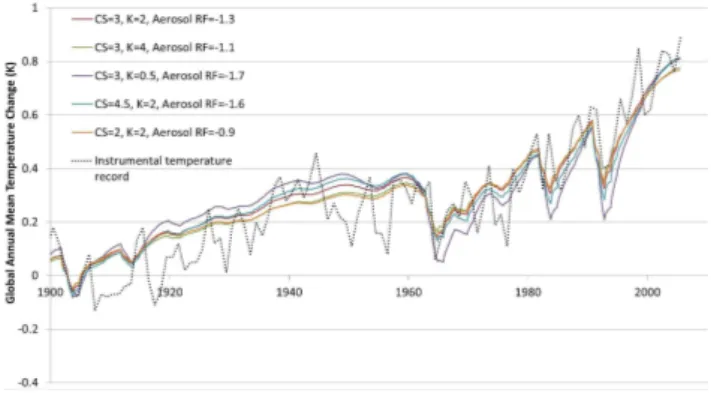
Fig. B1.Modeled and observed historic global mean surface tem-perature change. The historic temtem-perature series is taken from NASA GISS (2012). CS = climate sensitivity (Kelvins per CO2 equivalent doubling),K= the vertical heat diffusivity (cm2s−1). The aerosol forcing is given in W m−2for the year 2005. Historic estimates for the aerosol forcing are scaled linearly with this value.
Table C1.GWP and IGTP values for CH4. K, the vertical heat
diffusivity, is given in cm2s−1and CS, the climate sensitivity, is given in Kelvins per CO2equivalent doubling.
Time GWP IGTP
horizon CS = 3 CS = 4.5 CS = 2 CS = 3 CS = 3
K= 2 K= 2 K= 2 K= 4 K= 0.5
20 72 77 78 76 77 76
100 25 29 30 27 29 28
500 8 8 9 8 9 8
Appendix B
Modeling historic temperatures
Our UDEBM was run using historic radiative forcing data from the representative concentration pathway scenarios (see Meinshausen et al., 2011b) using different combinations of values for the climate sensitivity (CS), the vertical heat dif-fusivity (K) and the total radiative forcing from aerosols. It can be seen in Fig. B1 that the model fairly well reproduces the historic global mean surface temperature change over the period 1900–2005 (as estimated by NASA GISS, 2012) for each set of parameter combinations. When changing either the climate sensitivity or the vertical heat diffusivity, changes in the aerosol forcing are required to maintain a good fit with historic temperatures. There is significant uncertainty in the aerosol forcing, but our assumptions are well within the esti-mated range (Forster et al., 2007).
Appendix C
IGTP and GWP values
In Tables C1–C3, we summarize the GWP and IGTP values for CH4, N2O and SF6for different assumptions on the
cli-mate sensitivity and effective vertical heat diffusivity.
Table C2.GWP and IGTP values for N2O. K, the vertical heat
diffusivity, is given in cm2s−1and CS, the climate sensitivity, is given in Kelvins per CO2equivalent doubling.
Time GWP IGTP
horizon CS = 3 CS = 4.5 CS = 2 CS = 3 CS = 3
K= 2 K= 2 K= 2 K= 4 K= 0.5
20 289 284 283 285 284 284 100 298 301 301 300 301 300 500 153 162 166 160 165 158
Table C3.GWP and IGTP values for SF6.K, the vertical heat
dif-fusivity, is given in cm2s−1and CS, the climate sensitivity, is given in Kelvins per CO2equivalent doubling.
Time GWP IGTP
horizon CS = 3 CS = 4.5 CS = 2 CS = 3 CS = 3
K= 2 K= 2 K= 2 K= 4 K= 0.5
20 16 200 15 800 15 700 15 800 15 800 15 800 100 22 800 22 100 21 900 22 300 22 000 22 300 500 32 600 32 000 31 800 32 200 31 900 32 300
Appendix D
Demonstrating the asymptotic equivalence between IGTP and GWP
Let us assume the following simple model of the climate sys-tem with thermal inertia:
CdT
dt =F (t )−T /λ (D1)
whereC is the thermal inertia of the layer that should be heated,F (t )the radiative forcing,T the increase in temper-ature andλthe climate sensitivity (as above). Assume now that one kg of gasXis emitted, and that it decays exponen-tially with a life time ofτx,Fx(t )=Fxe−t /τx. We then obtain the temperature response to a pulse emission of gasXas TPx(t )=
τxλFx τx−λC
e−t /τx−e−t /λC. (D2) Integrating over the temperature response gives
H
Z
0
TPx(t )dt =
τxλFx τx−λC
n
τx
1−e−H /τx
−λC1−e−H /λCo. (D3)
temperature response is equal to the equilibrium increase in the atmospheric mass of gasXmultiplied by the forcing per kg multiplied by the climate sensitivity, i.e.τxλFx.
For CO2, the atmospheric “decay” function is somewhat
more complicated. We assume that it can be approximated by a sum of exponential functions and a constant term (see Forster et al., 2007), so that the radiative forcing at time t from the emission of kg of CO2at time 0 is equal to
FCO2(t )=FCO2 α0+
3
X
i=1
αie−t /τCO2,i
!
. (D4)
If so, the temperature following a pulse emission would be TP,CO2(t )=λFCO2
n
α0
1−e−λCt
+
3
X
i=1
αiτi τi −λC
e−
t
τi −e−λCt
)
. (D5)
Integrating over the temperature response gives H
Z
0
TP,CO2(t )dt =λFCO2
n
α0
H+Cλe−λCH
−1
+
3 X
i=1
αiτi
τi−λC
τi
1−e−Hτi
−λC1−e−H
λC
)
.(D6) Now calculate IGTP/GWP in the limitH−>∞
lim H→∞ IGTP(H ) GWP(H ) = lim H→∞ τx λFx τx−λC τx
1−e−τxH
−λC
1−e−λCH
λFCO2
(
α0
H+Cλ
e−H λC−1
+ 3 P i=1 αi τi τi−λC τi
1−e−Hτi
−λC
1−e−H
λC )
τxFx
1−e−τxH
FCO2
(
α0H+
3
P i=1
αiτi
1−e−Hτi )
=1.(D7)
Acknowledgements. Financial support from the Swedish Energy Agency and Carl Bennet AB is gratefully acknowledged.
Edited by: K. Keller
References
Azar, C. and Johansson, D. J. A.: Valuing the non-CO2
cli-mate impacts of aviation, Climatic Change, 111, 559–579, doi:10.1007/s10584-011-0168-8, 2012.
Baker, M. B. and Roe, G. H.: The shape of things to come: why is climate change so predictable?, J. Climate, 22, 4574–4589, 2009. Fisher, D. A., Hales, C. H., Wang, W.-C., Ko, M. K. W., and Sze, N. D.: Model calculation on the relative effects of CFCs and their replacements on global warming, Nature, 344, 513–516, 1990.
Forster, P., Ramaswamy, V., Artaxo, P., Berntsen, T., Betts, R., Fa-hey, D. W., Haywood, J., Lean, J., Lowe, D. C., Myhre, G., Nganga, J., Prinn, R., Raga, G., Schulz, M., and Van Dorland, R.: Changes in Atmospheric Constituents and in Radiative Forc-ing, in: Climate Change 2007: The Physical Science Basis. Con-tribution of Working Group I to the Fourth Assessment Report of the Intergovernmental Panel on Climate Change, edited by: Solomon, S., Qin, D., Manning, M., Chen, Z., Marquis, M., Av-eryt, K. B., Tignor, M., and Miller, H. L., Cambridge University Press, Cambridge, UK and New York, NY, USA, 2007. Gillet, X. and Matthews, H. D.: Accounting for carbon cycle
feed-backs in a comparison of the global warming effects of green-house gases, Environ. Res. Lett., 5, 034011, doi:10.1088/1748-9326/5/3/034011, 2010.
Hansen, J., Russell, G., Lacis, A., Fung, I., Rind, D., and Stone, P.: Climate Response Times: Dependence on Climate Sensitivity and Ocean Mixing, Science, 229, 857–859, 1985.
Hansen, J., Sato, M., Ruedy, R., Nazarenko, L., Lacis, A., Schmidt, G. A., Russell, G., Aleinov, I., Bauer, M., Bauer, S., Bell, N., Cairns, B., Canuto, V., Chandler, M., Cheng, Y., Del Genio, A., Faluvegi, G., Fleming, E., Friend, A., Hall, T., Jackman, C., Kel-ley, M., Kiang, N., Koch, D., Lean, J., Lerner, J., Lo, K., Menon, S., Miller, R., Minnis, P., Novakov, T., Oinas, V., Perlwitz, Ja., Perlwitz, Ju., Rind, D., Romanou, A., Shindell, D., Stone, P., Sun, S., Tausnev, N., Thresher, D., Wielicki, B., Wong, T., Yao, M., and Zhang, S.: Efficacy of Climate Forcings, J. Geophys. Res., 110, D18104, doi:10.1029/2005JD005776, 2005.
IPCC:Report of the IPCC Expert meeting on the Sci-ence of Alternative Metrics 18-20 March 2009, Oslo, available at http://www.ipcc.ch/pdf/supporting-material/ expert-meeting-metrics-oslo.pdf (last access: 5 February 2012), 2009.
Johansson, D. J. A.: Temperature stabilization, ocean heat uptake and radiative forcing overshoot profiles, Climatic Change, 108, 107–134, 2011.
Johansson, D. J. A.: Economics- and Physical-Based Metrics for Comparing Greenhouse Gases, Climatic Change, 110, 101–121, 2012.
Lashof, D. A. and Ahuja, D. R.: Relative contributions of green-house gas emissions to global warming, Nature, 344, 529–531, 1990.
Manne, A. S. and Richels, R. G.: An alternative approach to es-tablishing trade-offs among greenhouse gases, Nature, 410, 675– 677, 2001.
Meinshausen, M., Raper, S. C. B., and Wigley, T. M. L.: Emulat-ing coupled atmosphere-ocean and carbon cycle models with a simpler model, MAGICC6 – Part 1: Model description and cal-ibration, Atmos. Chem. Phys., 11, 1417–1456, doi:10.5194/acp-11-1417-2011, 2011a.
Meinshausen, M., Smith, S. J., Calvin, K. V., Daniel, J. S. Kainuma, M. L. T., Lamarque, J.-F., Matsumoto, K., Montzka, S. A., Raper, S. C. B., Riahi, K., Thomson, A. M., Velders, G. J. M., and van Vuuren, D.: The RCP Greenhouse Gas Concentrations and their Extension from 1765 to 2300, Climatic Change, 109, 213–241, 2011b.
Olivi´e, D. and Stuber, N.: Emulating AOGCM results using simple climate models, Clim. Dynam., 35, 1257–1287, 2010.
O’Neill, B. C.: The jury is still out on global warming potentials, Climatic Change, 44, 427–443, 2000.
Peters, G. P., Aamaas, B., Berntsen, T., and Fuglestvedt, J. S.: The integrated global temperature change potential (iGTP) and relationships between emission metrics, Environ. Res. Lett., 6, 044021, doi:10.1088/1748-9326/6/4/044021, 2011.
Raper, S. C. B., Gregory, J. M., and Osborn, T. J.: Use of an upwelling-diffusion energy balance climate model to simulate and diagnose A/OGCM results, Clim. Dynam., 17, 601–613, 2001.
Rodhe, H.: A comparison of the contribution of various gases to the greenhouse effect, Science, 248, 1217–1219, 1990.
Rotmans, J. and den Elzen, M. G. J.: A model-based approach to the calculation of global warming potentials (GWP), Int. J. Cli-matol., 12, 865–874, 1992.
Sarofim, M. C.: The GTP of methane: modeling analysis of temper-ature impacts of methane and carbon dioxide reductions, Envi-ron. Model. Assess., 17, 231–239, 2012.
Shine, K. P.: The global warming potential, The need for an inter-disciplinary retrial, Climatic Change, 96, 467–472, 2009. Shine, K. P., Derwent, R. G., Wuebbles, D. J., and Morcrette, J.
J.: Radiative forcing of climate, in: Climate change: the IPCC scientific assessment, edited by: Houghton, J. T., Jenkins, G. J., and Ephraums, J. J., Cambridge University Press, Cambridge, 1990.
Shine, K. P., Fuglestvedt, J. S., Hailemariam, K., and Stuber, N.: Al-ternatives to the global warming potential for comparing climate impacts of emissions of greenhouse gases, Climatic Change, 68, 281–302, 2005.