Scientific Drilling Into the San Andreas Fault Zone
—
An Overview of SAFOD’s First Five Years
by Mark Zoback, Stephen Hickman, William Ellsworth,
and the SAFOD Science Team
doi:10.2204/iodp.sd.11.02.2011Abstract
The San Andreas Fault Observatory at Depth (SAFOD) was drilled to study the physical and chemical processes controlling faulting and earthquake generation along an active, plate-bounding fault at depth. SAFOD is located near Parkfield, California and penetrates a section of the fault that is moving due to a combination of repeating microearth- quakes and fault creep. Geophysical logs define the San Andreas Fault Zone to be relatively broad (~200 m), contain-ing several discrete zones only 2–3 m wide that exhibit very low P- and S-wave velocities and low resistivity. Two of these zones have progressively deformed the cemented casing at measured depths of 3192 m and 3302 m. Cores from both deforming zones contain a pervasively sheared, cohesion-less, foliated fault gouge that coincides with casing deforma-tion and explains the observed extremely low seismic veloci-ties and resistivity. These cores are being now extensively tested in laboratories around the world, and their composi-tion, deformation mechanisms, physical properties, and rheological behavior are studied. Downhole measurements show that within 200 m (maximum) of the active fault trace, the direction of maximum horizontal stress remains at a high angle to the San Andreas Fault, consistent with other measurements. The results from the SAFOD Main Hole, together with the stress state determined in the Pilot Hole, are consistent with a strong crust/weak fault model of the San Andreas. Seismic instrumentation has been deployed to study physics of faulting—earthquake nucleation, propa-gation, and arrest—in order to test how laboratory-derived concepts scale up to earthquakes occurring in nature.
Introduction and Goals
SAFOD (the San Andreas Fault Observatory at Depth) is a scientific drilling project intended to directly study the physical and chemical processes occurring within the San Andreas Fault Zone at seismogenic depth. The principal goals of SAFOD are as follows: (i) study the structure and composition of the San Andreas Fault at depth, (ii) deter-mine its deformation mechanisms and constitutive proper-ties, (iii) measure directly the state of stress and pore pres-sure in and near the fault zone, (iv) determine the origin of fault-zone pore fluids, and (v) examine the nature and signif-icance of time-dependent chemical and physical fault zone processes (Zoback et al., 2007).
Detailed planning of a research experiment focused on drilling, sampling, and downhole measurements directly within the San Andreas Fault Zone began with an interna-tional workshop held in Asilomar, California in December 1992. This workshop highlighted the importance of deploying a permanent geophysical observatory within the fault zone at seismogenic depth for near-field monitoring of earthquake nucleation. Hence, from the outset, the SAFOD project has been designed to achieve two parallel suites of objectives. The first is to carry out a series of experiments in and near the San Andreas Fault that address long-standing questions about the physical and chemical processes that control deformation and earthquake generation within active fault zones. The second is to make near-field observations of earthquake nucleation, propagation, and arrest to test how laboratory-derived concepts about the physics of faulting
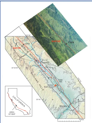
Figure 1. Map of the Parkfield segment of the San Andreas Fault showing the epicenters of the 1966 and 2004 Parkfield earthquakes and the SAFOD drillsite (Rymer et al., 2006). The air photo shows the terrain in the area of the SAFOD drill site and the epicenter of the 1966 Parkfield earthquake.
M I D
D LE
M O
U N
TA I N
C H
O L
A M
E H
I L L S
C H
O L
A M
E V
A L
L E Y
41 46
46
FRESNO CO
Cholame Parkfield
Gold Hill
2 0 0 4 E p i c e n t e r 1 9 6 6
35°52'30"
35°45' 36°00'
500
500
750
750
1000
1000
SAFOD 120°30'
120°2 2'3
0"
12 0°1
5' SAN ANDREAS FAULT
SOUTHWEST FRAKTURE ZONE
10 Km 0
AREA OF MAP
CA
L IFO
RN
I A
1 9 6 6
scale up to earthquakes occurring in nature. In the years following the Asilomar workshop, dozens of planning meetings were held to synthesize the research questions of highest scientific priority that were deemed to be operation-ally achievable. Numerous other meetings were also held related to site selection and to detailed operational plans for drilling, sampling, downhole measurements, and long-term monitoring.
When planning of the EarthScope initiative got underway at the National Science Foundation (NSF) in the late 1990s, the project was named SAFOD and became one of the three components of EarthScope along with the Plate Boundary Observatory (PBO) and USArray. In 2002, a 2.2-km-deep Pilot Hole was funded by the International Continental Scientific Drilling Program (ICDP) and was drilled at the SAFOD site. The main SAFOD project started when NSF funded the EarthScope proposal in 2003, with substantial cost sharing and operational support for SAFOD provided by the U.S. Geological Survey (USGS), ICDP, and other agen-cies.
The SAFOD operational plan was designed to address a number of first-order scientific questions related to fault mechanics in a hostile environment where the mechanically and chemically altered rocks in the fault zone are subject to high mean stress, potentially high pore pressure, and ele-vated temperature. Some of these questions are listed below.
• What are the mineralogy, deformation mechanisms, and
constitutive properties of fault gouge? Why do some
faults creep? What are the strength and frictional properties of recovered fault rocks at in situ conditions of stress, fluid pressure, temperature, strain rate, and pore fluid chemistry? What determines the depth of the shallow seismic-to-aseismic transition? What do mineralogical, geochemical, and microstructural analyses reveal about the nature and extent of water-rock interaction?
• What is the fluid pressure and permeability within and
adjacent to fault zones? Are there super-hydrostatic
fluid pressures within some fault zones, and through what mechanisms are these pressures generated and/or maintained? How does fluid pressure vary during deformation and episodic fault slip (creep and earthquakes)? Do fluid pressure seals exist within or adjacent to fault zones, and at what scales?
• What are the composition and origin of fault-zone fluids
and gases? Are these fluids of meteoric, metamorphic,
or mantle origin (or combinations of the three)? Is fluid chemistry relatively homogeneous, indicating pervasive fluid flow and mixing, or heterogeneous, indicating channelized flow and/or fluid compart- mentalization?
• How do stress orientations and magnitudes vary across
fault zones? Are principal stress directions and
magni-tudes different within the deforming core of weak fault zones compared to the adjacent (stronger) country rock, as predicted by some theoretical models? How does fault strength measured in the near field com-pare with depth-averaged strengths inferred from heat flow and regional stress directions? What is the nature and origin of stress heterogeneity near active faults?
• How do earthquakes nucleate? Does seismic slip begin
suddenly, or do earthquakes begin slowly with accel-erating fault slip? Do the size and duration of this pre-cursory slip episode, if it occurs, scale with the magni-tude of the eventual earthquake? Are there other precursors to an impending earthquake, such as changes in pore pressure, fluid flow, crustal strain, or electromagnetic field?
• How do earthquake ruptures propagate? Do they
propa-gate as a uniformly expanding crack, as a slip pulse, or as a sequence of slipping high-strength asperities? What is the effective (dynamic) stress during seismic faulting? How important are processes such as shear heating, transient increases in fluid pressure, and fault-normal opening modes in lowering the dynamic frictional resistance to rupture propagation?
• How do earthquake source parameters scale with
magni-tude and depth? What is the minimum size earthquake
that occurs on faults? How is long-term energy release rate partitioned between creep dissipation, seismic radiation, dynamic frictional resistance, and grain size reduction (determined by integrating fault zone monitoring with laboratory observations on core)?
• What are the physical properties of fault-zone materials
and country rock (seismic velocities, electrical
resistiv-ity, densresistiv-ity, porosity)? How do physical properties from
core samples and downhole measurements compare with properties inferred from surface geophysical observations? What are the dilational, thermoelastic, and fluid-transport properties of fault and country rocks, and how might they interact to promote either slip stabilization or transient over-pressurization dur-ing faultdur-ing?
• What processes control the localization of slip and strain?
Are fault surfaces defined by background microearth-quakes and creep the same? Would active slip surfaces be recognizable through core analysis and downhole measurements in the absence of seismicity and/or creep?
repeating microearthquakes, M3 and smaller, occurring on the fault at depths of 2–12 km (Waldhauser et al., 2004). The Parkfield segment of the fault hosts the well-studied seven M6 earthquakes that have ruptured since 1857 (Bakun and McEvilly, 1984). Slip distributions for the last two Parkfield earthquakes—on 28 June 1966 and 28 September 2004— determined using geodetic measurements, indicate that the ruptures terminated a few kilometers southeast of SAFOD (Murray and Langbein, 2006; Harris and Arrowsmith, 2006 and papers therein).
Beginning at the Asilomar meeting, site selection com-mittees winnowed down eighteen potential sites to four, and eventually the northwest end of Parkfield segment was se-lected. The geology seemed ideal since Salinian granite on the west side of the fault was expected to be juxtaposed against Franciscan melange on the east side, so a major geo-logic discontinuity was expected when crossing the fault at depth. Also, the San Andreas Fault is quite active in the area, exhibiting a combination of aseismic creep and frequent microearthquakes that would help define the exact location of the active fault trace at depth. In addition, more is known about this section of the San Andreas than any other,due to the intense interest in capturing a M~6 earthquake within a dense network of instrumentation.
After selecting the Parkfield segment of the San Andreas for the SAFOD experiment, the next question of particular
importance was where exactly to site the borehole. The site chosen (Fig. 1) was selected near Middle Mountain because re- peating microearthquakes could be reached at the shallowest depth possible close to the fault to limit the horizontal reach of the borehole. As shown in the photo inset of Fig. 1, the selected site is a broad, relatively flat area where a 5-acre drill pad could be constructed 1.8 km southwest of the surface trace of the fault. Once this area was identified, a num-ber of detailed geophysical and geologic site studies were carried out to allow results from SAFOD to be placed in the appropriate geological and geophysical context and to assure that the drill site selected would not encounter any large-scale faults or struc-fault has low frictional strength: the absence of
frictionally-generated heat, and the orientation of the maximum principal stress in the crust adjacent to the fault. A large number of heat flow measurements show no evidence of frictionally generated heat adjacent to the San Andreas Fault (Lachenbruch and Sass, 1980, 1992; Williams et al., 2004), which implies that shear motion along the fault is resisted by shear stresses approximately a factor of five less than fric-tional strength of the adjacent crust. This observation is sometimes referred to as the San Andreas stress/heat flow paradox. Saffer et al. (2003) showed that it is highly unlikely that topographically driven fluid flow has an appreciable effect on these heat flow measurements, indicating that the lack of frictionally-generated heat in the vicinity of the San Andreas Fault is indeed indicative of low aver-age shear stress levels acting on the fault at depth. In addition to the heat flow data, the orientation of principal stresses in the vicinity of the fault also indicates that right-lateral strike slip motion on the fault occurs in response to low levels of shear stress (Zoback et al., 1987; Mount and Suppe, 1987; Oppenheimer et al., 1988).
Why Parkfield? SAFOD is located in central California (Fig. 1) near the town of Parkfield, at the transition between the locked (i.e., seismogenic) portion of the fault to the southeast and the segment of the fault to the northwest where slip dominantly occurs by aseismic creep. The fault is seismically active around SAFOD with numerous sites of
Figure 2. Microearthquakes selected for targeting with SAFOD. [A] 3-D perspective view of the seismicity with respect to the path of the SAFOD borehole, with north pointing up, east to the right, and depth down (all axes in km). [B] View of the plane of the San Andreas Fault at about 2.7-km depth looking to the northeast. The red, blue, and green circles represent seismogenic patches of the San Andreas Fault that produce nearly identical, regularly repeating microearthquakes termed the San Francisco (SF), Los Angeles (LA), and Hawaii (HI) clusters, respectively. The point at which the SAFOD borehole passes through the central deforming zone (CDZ) is shown by the asterisk. [C] Cross-sectional view of these earthquakes looking to the northwest, parallel to the San Andreas Fault, including the trajectory of the SAFOD borehole and the principal faults associated with the damage zone shown in Figs. 3 and 4. Note that the HI events occur about 100 m below the fault intersection at 3192 m (measured depth), indicating that the HI microearthquakes occur on the southwest deforming zone (SDZ). The SF and LA sequences occur on the northwest bounding fault (NBF), as discussed in the text.
D
C
B
A
SF
LA 1
1
1 2
2
2 3
3
3
4
1985 1990 1995 2000 2005 2010
SF
Year
Magnitude
1985 1990 1995 2000 2005 2010
LA
Year
Magnitude
1985 1990 1995 2000 2005 2010
HI
Year
Magnitude
0
0
0
1
1
1
2
2
2
3
3
3
M 6
400−2900 300 200 100 0 −100m
−2800
−2700
−2600
−2500
−2400
Fault Plane View
Depth (m)
SF LA
SF LA
HI
Distance from Fault Intersection (N 45 W)
*
CDZ
Intersection Point
1100 1200 1300 1400 1500 1600m
−2900
−2800
−2700
−2600
−2500
−2400
Distance from SAFOD Wellhead (N 45 E)
Depth (m)
SF
LA
HI
Fault Normal View
3192 SDZ 3302
CDZ 3413
SAFOD Obser
vatory
SAFOD Main
Borehole Damage
Zone
most of the two actively deforming fault traces identified in the SAFOD crossing. The microearthquake locations shown in Fig. 2 were determined utilizing subsurface recordings of these earthquakes from various geophone deployments in the SAFOD borehole along with surface recordings from the dense Parkfield Area Seismic Observatory (PASO; Thurber et al., 2004). This said, although the accuracy of location of HI is good (being determined by a seismometer deployed in SAFOD directly above the events), the location of SF and LA with respect to HI is relatively uncertain.
SAFOD Pilot Hole
In preparation for SAFOD, a 2.2-km-deep, near-vertical Pilot Hole was drilled and instrumented at the SAFOD site in the summer of 2002. The Pilot Hole was rotary drilled with a 22.2-cm bit, and cased with 17.8-cm outside diameter (OD) steel casing. The Pilot Hole is currently open to a depth of 1.1 km (explained below) and available for instrument testing, cross borehole experiments, and other scientific studies. Hickman et al. (2004) present an overview of the Pilot Hole experiment.
There were a number of important technical, operational, and scientific findings in the Pilot Hole. These include geo-logic confirmation of the depth at which the Salinian gran-ites and granodiorgran-ites would be encountered (Fig. 3), and calibration of geophysical models with direct measurements of seismic velocities (Boness and Zoback, 2004; Thurber et al., 2004), resistivity (Unsworth and Bedrosian, 2004), den-sity, and magnetic susceptibility (McPhee et al., 2004). In tural complexities in the near surface.
These studies included an extensive microearthquake survey, high-resolution seismic reflection/refraction profiling, magnetotelluric profiling, ground and closely-spaced aeromagnetic surveys, gravity surveys, and geologic mapping.
The repeating microearthquakes pro-vide targets on the fault plane at depth to guide the drilling trajectory (Fig. 2A) into the microearthquake zone at less than 3 km depth. Another reason for choosing this site is that there are three sets of repeating M~2 earthquakes in the target area. Surrounding these patches, fault slip occurs through aseismic creep. In a view normal to the plane of the San Andreas Fault Zone at 2.65 km depth (Fig. 2B), we see the source zones asso-ciated with these three patches (scaled for a ~10-MPa stress drop). The seismograms from each of these source zones are essentially identical (Nadeau et al., 2004), and cross-correlation demonstrates that within ±10 m uncertainty these events are
located in exactly the same place on the faults (F. Waldhauser, pers. comm.).
As shown in Fig. 2B, we refer to the shallower source zone in the direction of San Francisco as the SF events, and the adjacent source zone in the direction of Los Angeles as LA events. Note that the SF and LA patches are adjacent to each other; it is common for LA events to occur immediately after SF events as triggered events. As seen in Fig. 2B, the third cluster of events (in green) occurs on a fault plane to the southwest of that upon which the SF and LA events occur. As this cluster of events is to the southwest of the other two clusters, these are referred to as the Hawaii (HI) events.
The time sequences of the three clusters of repeating earthquakes are shown in Fig. 2C. Note that prior to the M6 Parkfield earthquake of September 2004, each of the three clusters produced an event every ~2.5–3.0 years. Following the Parkfield earthquake, the frequency of the events increased dramatically, apparently due to accelerated creep on this part of the fault resulting from stress transfer from the M~6 main-shock. Following this flurry of events the fre-quency of the repeaters slowed down and is presently in the process of returning to the background rate exhibited prior to the main shock. Similar behavior has been seen elsewhere along the San Andreas Fault system in California (Schaff et al., 1998).
Note in Fig. 2B that the HI events occur about 100 m below the fault intersection at 3192 m (measured depth), indicating that the HI microearthquakes occur on the
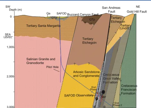
southwestern-Figure 3. Simplified geologic cross-section parallel to the trajectory of the San Andreas Fault Observatory at Depth (SAFOD) borehole. The geologic units are constrained by surface mapping and the rock units encountered along both the main borehole and the pilot hole. The black circles represent repeating microearthquakes. The three notable fault traces associated with the San Andreas Fault damage zone (SDZ, CDZ, and NBF) are shown in red. The depth at which the SAFOD observatory is deployed is shown.
Salinian Granite and
Granodiorite
Tertiary Etchegoin
Cretaceous Great Valley
Formation
Cretaceous
Franciscan Formation
SAFOD
Tertiary
(Undiff.)
Arkosic Sandstone and Conglomerate
? ?
? ?
?
End of Phase 1 Pilot Hole
SW NE
QTp QTp
Tertiary Santa Margarita
Qa
San Andreas Fault
3,000 2,000 1,000 0 Depth (m)
SAFOD Observatory
SEA LEVEL
Gold Hill Fault Buzzard Canyon Fault
? ?
?
?
Arkosic Sandstone and Conglomerate
SDZ CDZ
NBF
End Phase 1
End Phase 2
carried out during the summer of 2004, involved rotary drill-ing vertically to a depth of ~1.5 km, then steerdrill-ing the well at an angle ~60° from vertical toward the repeating microearth-quakes described above (Fig. 3). Note that these earthqua-kes occur to the southwest of the surface trace of the San Andreas, which indicates that at this location the fault dips steeply to the southwest. By design, Phase 1 ended just outside the San Andreas Fault Zone so that relatively large-diameter (24.4 cm) steel casing could be deployed and cemented in place prior to drilling through the active fault zone where substantial drilling problems might be encoun-tered. Results from a number of scientific studies carried out during Phase 1 were needed to establish key engineering parameters (such as the optimal density of the drilling mud) for drilling through the San Andreas Fault during Phase 2 (Paul and Zoback, 2008).
Phase 2 was carried out during the summer of 2005. A relatively large-diameter (21.6 cm) hole was rotary drilled across the San Andreas Fault Zone (Fig. 3). While many of the key scientific objectives of SAFOD require recovery of core samples from the fault zone, we decided to rotary drill through the fault zone for several reasons. First, rotary drill-ing is far more robust than core drilldrill-ing. If the borehole turned out to be unstable due to the rock being highly bro-ken up and chemically altered by faulting (which turned out to be the case), and/or high pore pressure was encountered in the fault zone at depth (which was not the case), it would be much easier to deal with such problems and ensure that we would make it all the way across the fault zone with rotary drilling rather than core drilling. Second, rotary drilling pro-duces a larger diameter hole than core drilling. This was needed to carry out a wide range of sophisticated geophysi-cal measurements (especially well logs) in the fault zone with equipment developed for the petroleum industry. When drilling problems are encountered during coring, it is com-mon for the drill rod to get stuck in the hole. When this hap-pens, the sizes of drill bit and coring rods are reduced so that coring can continue through the bottom of the stuck coring rod. Consequently, the diameter of core holes start relatively small and potentially reduces rapidly. As illustrated below, these geophysical measurements proved to be critical for defining the nature of the overall fault zone as well as the active shear zones within it. The final reason for maintaining a relatively large-diameter hole was related to deployment of the observatory instrumentation in the fault zone after drill-ing. It was important to complete the well with sufficiently large-diameter casing (17.8 cm) to allow a suite of seismo-meters and acceleroseismo-meters to be deployed in the borehole.
Phase 3 was carried out during the summer of 2007; it involved drilling multi-lateral holes which start by milling a hole in the side of the steel casing in the Main Hole. By using multilateral drilling to create secondary holes at optimal locations (a technology that is now commonplace in the petroleum industry), we could direct coring efforts within the most important intervals identified during Phase 2. By addition, stress measurements in the Pilot Hole were found
to be consistent with the strong crust/weak fault model discussed above (Boness and Zoback, 2004; Hickman and Zoback, 2004). In other words, stress differences in the crust 1.8 km from the San Andreas were high and consistent with Byerlee’s law, whereas the direction of maximum horizontal stress in the lower part of the hole was nearly orthogonal to the San Andreas Fault. Furthermore, heat flow measured to 2.2 km depth (Williams et al., 2004) was found to be consis-tent with shallower data in the region, confirming that the shallow measurements are not affected by heat transport and thus indicate no frictional heat being generated by slip on the San Andreas Fault. Hence, the Pilot Hole confirmed that the SAFOD site was indeed an appropriate site for examining possible explanations for the San Andreas stress/ heat flow paradox.
After drilling and downhole measurements were complet-ed, the Pilot Hole was used for deployment of a vertical seis-mic array to record naturally occurring seis-microearthquakes and to image some of the large-scale structures at depth in the vicinity of the San Andreas (Chavarria et al., 2003; Oye and Ellsworth, 2007). This array was also used to record sur-face explosions as an important part of the effort to constrain seismic velocities in the vicinity of the borehole for achiev-ing the best possible locations of the target earthquakes (Roecker et al., 2004). Use of the Pilot Hole for experiments such as cross-hole monitoring of time-varying shear velocity (Niu et al., 2008) will continue to produce interesting results for years to come. From an engineering perspective, by es-tablishing the depth to basement and the conditions affect-ing drillaffect-ing in the upper sedimentary section, the Pilot Hole helped establish key aspects of the engineering design of the upper part of the SAFOD Main Hole.
SAFOD Main Borehole
A great deal of engineering and operational planning went into SAFOD, since drilling, coring, and scientific measure-ments in the hostile environment of an active, plate-bounding fault zone had never been attempted before. A number of sci-entific workshops were held on drilling and downhole measurements, fault zone monitoring, and core handling. In addition, a formal advisory structure was established to take advantage of the knowledge and experience of scientists from universities, the USGS and U.S. Department of Energy (DOE) national labs, and the petroleum industry. A Scientific Advisory Board provided high-level scientific guidance for the project. Technical panels on drilling, coring, and safety, downhole measurements, core handling, and downhole monitoring provided invaluable advice on literally hundreds of issues affecting how the project was eventually carried out.
design, the samples and physical property measurements of the fault zone obtained during Phase 2 were not the only information available to us to guide Phase 3 coring opera-tions. Due to accelerated fault creep following the 2004 earthquake, the casing deployed across the fault zone follow-ing Phase 2 was deformed at specific places which directly indicated the active strands of the San Andreas at depth.
Phase 1 and 2 Operational Overview. As mentioned above,
Phases 1 and 2 were rotary drilled. In order to obtain as much scientific information as possible during drilling, a comprehensive real-time sampling of drill cuttings, drilling fluid, and formation gases in the drilling mud was carried out. Following each phase, a suite of geophysical measure-ments was obtained, and a limited amount of coring was done at each depth where casing was set.
As can be seen in Fig. 3, the Main Hole starts vertically and at approximately 1.5 km depth; directional drilling tech-niques were employed to slowly deviate the borehole (even-tually at an angle ~60° from vertical) in order to intersect the San Andreas Fault in the vicinity of the repeating target earthquakes. A wide range of information is available online including that related to real-time operations (Table 1). One source of information that provides a convenient overview of Phases 1 and 2 are the Commercial Mud Logs, which deliver also lithologic descriptions of the drill cuttings. Numerous faults were observed in all of the rock units drilled through (Boness and Zoback, 2006). Bradbury et al. (2007) de- scribed the mineralogy of drill cuttings in terms of fault zone composition and geologic models.
The first geologic surprise that occurred during Phase 1 was that soon after deviating the borehole toward the San Andreas Fault, we drilled through a major fault zone at a ver-tical depth of 1.8 km (interpreted to be the Buzzard Canyon Fault, see Fig. 3) as we passed out of the Salinian granitic basement rocks and into previously unknown arkosic sand-stones and conglomerates, with some interbedded shales (Boness and Zoback, 2006; Solum et al., 2006). In general, these are strongly cemented rocks that are likely derived from weathering of Salinian granites and granodiorites. Draper Springer et al. (2009) described this section in some detail and pointed to at least a dozen significant faults within
it. While they argued for this being a depositional unit formed proximal to the Salinian granite, they suggested that it may have been translated along strike by as much as ~300 km. One reason this unit had not been identified by geo-physical surveys through the site area is that these rocks are so strongly cemented that their seismic velocities and resis-tivity do not vary significantly from the fractured Salinian granites and granodiorites (Boness and Zoback, 2006).
At a measured depth along the borehole of 1460 m (while still drilling in the granite/granodiorite), a planned pause in drilling took place to run steel casing into the hole before further drilling. Prior to casing the hole, a suite of geophysi-cal logs was run. After running the casing into the hole and cementing it in place, 7.9 meters of fractured and faulted hornblende-biotite granodiorite core were obtained. In addi-tion, fluid samples were taken at this depth, and a small-scale hydraulic fracturing experiment was done to constrain the magnitude of the least principal stress.
After drilling resumed, Phase 1 continued to a total verti-cal depth of 2507 m. As shown in Fig. 3, Phase 1 drilling ended in the arkosic sandstone/conglomerate section. At the end of Phase 1 drilling a second suite of geophysical logs was run. Boness and Zoback (2006) presented a summary of the Phase 1 lithologies and geophysical logs. After cementing steel casing into the wellbore, an 11.6-m core—composed of fractured and faulted arkosic sandstone and conglomerate— was obtained, and fluid sampling was then performed.
One mishap that occurred during Phase 1 was a collision between the Main Hole and the Pilot Hole at 1.1 km depth. Because of the respective layouts of the drilling equipment used for the Pilot and Main Holes, the wellheads of the two boreholes were located only 6.75 m apart. In an attempt to avoid collision of the two holes at depth, repeated gyroscopic surveys of both holes and directional drilling were used. This is commonplace in the oil industry where dozens of wells are often drilled from the same platform or drill site. After the incident, we learned that the collision was caused by poor calibration of one set of the gyroscopic survey in-struments. The lasting impact of the hole collision is loss of access to the lower part of the Pilot Hole, as the casing is severely damaged at 1.1 km depth. The Pilot Hole seismic
Table 1. Accessing SAFOD Data Online.
Description URL
EarthScope Data Portal – Information about and access to all SAFOD EarthScope data
and samples http://www.earthscope.org
IRIS DMC – SAFOD seismological data archive including assembled data sets http://www.iris.edu/hq Northern California Earthquake Data Center – Earthquake catalogs and seismograms for
all local networks including SAFOD, High-Resolution Seismic Network (HRSN) and NCSN http://www.ncedc.org/safod/ ICDP Web site – Direct access to all data obtained as drilling, logging and coring
operations were underway. Bibliography of SAFOD papers. http://safod.icdp-online.org
Online Core Viewer – Photographs of all cores and samples taken for scientific study ht tp:// w w w.ear thscope.org/data /safod _core _ viewer
Phase 3 Core Atlas – High-resolution images of Phase 3 cores as well as preliminary lithologic and microstructural descriptions
http://www.icdp-online.org/upload/projects/safod/ phase3/Core_Photo_Atlas_v4.pdf
array was also lost as a consequence of the accident; the lowermost twenty-five levels were severed during the inter-section, and the remaining seven levels were decommis- sioned in the spring of 2005 when an unsuccessful attempt was made to regain access to the Pilot Hole below the inter-section.
During the nine-month hiatus (September 2004 to June 2005) between the end of Phase 1 and the beginning of Phase 2, a number of seismometers were deployed in the SAFOD Main Hole as part of an instrument testing program for eventual deployment of the SAFOD observatory. A num-ber of shots were set off while the seismometers were in the borehole to better constrain the velocity model and reduce uncertainty in the location of the target earthquakes. In addi-tion, an eighty-level, 240-component seismic array was made available by Paulsson Geophysical Services, Inc. (PGSI) and recorded by Geometrics at no cost to the project. This array was deployed in the borehole for a period of five weeks in order to test its suitability for recording microearthquakes and to record additional shots for structural imaging (Chavarria and Goerrtz, 2007). In addition to recording microearthquakes and shots during this period, a tectonic (i.e., non-volcanic) tremor was recorded on this array. The tremor occurred in the lower crust directly below the sur-face trace of the San Andreas Fault for at least 70 km to the northwest and 80 km to the southeast of SAFOD (Shelly and Hardebeck, 2010). The likely source of the tremor recorded by the PGSI array was in the vicinity of the energetic tremor source near Cholame (Nadeau and Dolenc, 2005) near the base of the crust (~25 km; Shelly and Hardebeck, 2010).
As shown in Fig. 3, Phase 2 drilling passed from the arkosic sandstones and conglomerates into mudstones and shales at a depth of 2600 m, and at a position ~500 m southwest of the surface trace of the San Andreas Fault. Microfossil evidence from core obtained at the bottom of the Phase 2 hole indicates that these formations are part of the Cretaceous Great Valley sequence, which was deposited on the North American plate in a forearc environment at a time when subduction was occurring along the western margin of California (K. McDugall, pers. comm., 2005). In the long-term geologic sense, the contact between the Salinian-derived arkosic sandstones and conglomerates and the Great Valley formation is the boundary between the Pacific and North American plates. As shown by progressive deformation of the casing discussed below (Fig. 4), the south-westernmost of the active traces of the San Andreas Fault Zone at depth is located several tens of meters to the northeast of this geologic boundary.
No evidence was found that we had encountered the Franciscan Formation in the borehole, even though it is exposed at the surface about 600 m east of the San Andreas Fault (Fig. 3), and was predicted by several of the geophysi-cal surveys conducted in advance of drilling. However, there is evidence of serpentinite directly within the fault zone
asso-ciated with either the Coast Range ophiolite or Franciscan formation. Hence, there is likely serpentinite in contact with the San Andreas along strike and/or at greater depth. A rea-sonable conceptual model is that slivers of Great Valley and the Franciscan are intermixed at depth along the fault, just as they are found in surface exposures at several locations in central California.
Rotary drilling through the San Andreas Fault during Phase 2 was accomplished with no small amount of diffi-culty—some caused by the fault zone, some caused by unre-lated operational problems (for example, the top drive, an extremely important component of the drill rig, broke and was inoperable for two weeks). We also noted a considerable degree of time-dependent wellbore failure (Paul and Zoback, 2008), especially after passing through the active traces of the San Andreas Fault Zone. An appreciable amount of time was required to clean the hole through wash and ream ope-rations. In fact, the combined result of time-dependent wellbore instabilities and a mistake by the drilling crew resulted in the drillstring being stuck in the hole for four days at a vertical depth of 2800 m. Despite these problems, drilling across the entire fault zone was successfully achie-ved. Comprehensive cuttings and gases were sampled over the entire Phase 2 interval (Table 2), and a number of geo-physical measurements were made in real-time as drilling across the fault zone was underway (Run 4, Table 3). After the hole was drilled, a comprehensive suite of geophysical logs was obtained, and fifty-two 19-mm-diameter side-wall cores were obtained in the open hole (Run 4, Table 3). After the hole was cased and cemented, 3.9 meters of core (mud-stones of the Great Valley formation, mentioned above) were obtained from the very bottom of the hole.
Phase 1 and 2 Real-time Sampling. Drill cuttings and
for-mation gases were collected in real time as drilling was taking place. Drill cuttings were collected every 3 m and pre-served in both washed and unwashed states, and larger vol-umes of cuttings were collected at less frequent intervals, as were samples of the drilling mud. Table 2 summarizes the cuttings samples, side-wall cores, and the three cores ob-tained after casing was cemented into place at various depths. Photographs, detailed descriptions, and other infor-mation about the extensive collection of cuttings are avail-able online (Tavail-able 1). A summary of the lithologies encoun-tered during Phases 1 and 2 is provided by Solum et al. (2006) and Bradbury et al. (2007), principally based on X-ray diffraction (XRD) analyses and optical analyses of mineral-ogy and texture of the cuttings, augmented by the spot and sidewall cores.
that the San Andreas Fault has very low permeability and hydrologically separates the Pacific and North American plates (Wiersberg and Erzinger, 2008).
Downhole Measurements. A wide range of downhole
measurements was carried out as part of SAFOD Phases 1 and 2 (Table 3). As the structure and properties of the San Andreas Fault Zone are of most importance, we show in Fig. 4A a summary of the geophysical logs from Phase 2 along with some of the main lithologic units encountered.
An approximately 200-m-wide damage zone of
anoma-lously low P- and S-wave velocities and low resistivity
(Fig. 4A) is interpreted to be the result of both physical damage and chemical alteration of the rocks due to faulting as well as the unusual, fault-related minerals (discussed above) that were noted during drilling. There are also a num-ber of localized zones where the physical properties are even more anomalous. Repeated measurements of the shape of the steel casing deployed in the borehole revealed that the steel casing was being deformed by fault movement in at least two places. Figure 4C shows the casing radius (as measured using a 40-finger caliper) as a function of position around the hole. While the amount of deformation associated with the 3302-m shear zone is more pronounced than the Andreas Fault Zone (Solum et al., 2006). Moore and Rymer
(2007) demonstrated that some of the serpentinite in the fault zone has been altered to talc, an unusual mineral in that it has exceptionally low frictional strength and is thermo-dynamically stable over the range of depths and pressures characteristic of the upper crust in this region. They spec-ulated that if talc is widespread in the fault zone, it could explain both the strength of the fault and its creeping behav-ior.
Gases coming into the well as the borehole was being drilled yielded a great deal of useful data. This technology, in which gas is separated from the drilling mud as it comes to the surface, was also used in the Pilot Hole where gas anoma-lies correlated with shear zones in the granite/granodiorite (Erzinger et al., 2004). During Phases 1 and 2, implementa-tion of this technology showed a number of important corre-lations with major faults and geologic boundaries. One finding of particular interest reported by Wiersberg and Erzinger (2007) is that there is a marked difference in the concentration of 3He/4He across the San Andreas Fault. On
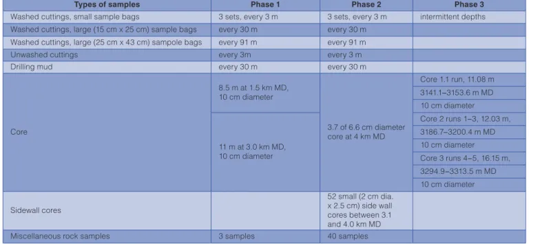
the southwest side of the fault this ratio is ~0.4, whereas on the northeast side of the fault it is ~0.9. This data and differ-ences in the relative concentrations of hydrogen, carbon dioxide, and methane on the two sides of the fault indicate Table 2. Summary of Physical Samples Obtained from SAFOD.
Types of samples Phase 1 Phase 2 Phase 3
Washed cuttings, small sample bags 3 sets, every 3 m 3 sets, every 3 m intermittent depths Washed cuttings, large (15 cm x 25 cm) sample bags every 30 m every 30 m
Washed cuttings, large (25 cm x 43 cm) sampole bags every 91 m every 91 m Unwashed cuttings every 3m every 3 m
Drilling mud every 30 m every 30 m
Core
8.5 m at 1.5 km MD, 10 cm diameter
3.7 of 6.6 cm diameter core at 4 km MD
Core 1.1 run, 11.08 m 3141.1–3153.6 m MD 10 cm diameter
11 m at 3.0 km MD, 10 cm diameter
Core 2 runs 1–3, 12.03 m, 3186.7–3200.4 m MD 10 cm diameter
Core 3 runs 4–5, 16.15 m, 3294.9–3313.5 m MD 10 cm diameter
Sidewall cores
52 small (2 cm dia. x 2.5 cm) side wall cores between 3.1 and 4.0 km MD Miscellaneous rock samples 3 samples 40 samples
Table 3. SAFOD Geophysical Logging Data.
Run Depth Range
(Measured Depth) Logging Technique Parameters Measured
Run 1 602.5–1443.5 m Open Hole, Wireline Density, porosity, gamma, caliper, resistivity, cross-dipole sonic velocity, FMI
Run 2a 1368–2030 m Open Hole, Wireline Density, porosity, gamma, caliper, resistivity, sonic velocity, FMI, UBI, ECS
Run 2b 1890–3043 m Open Hole, Pipe Conveyed Density, porosity, gamma, caliper, resistivity, sonic velocity, FMI Run 3 1356–3033 m Cased Hole, Wireline Sonic velociy, elemental chemistry, cement bond
Run 4 3045–3712 m Open Hole, Logging While Drilling Density, porosity, gamma, caliper, resistivity, FMI
Run 5 3045–3965 m Open Hole, Pipe Conveyed Density, porosity, gamma, caliper, resistivity, sonic velocity, FMI Runs 6–11* 2953–3815 m Cased Hole, Wireline Caliper, direction, temperature
(Fig. 1). Recent relocations of the SAFOD target earth- quakes indicate that the SF/LA cluster correlates with the fault at 3413 m, as shown in Fig. 2D (Thurber et al., 2010). This fault defines the northeastern edge of the damage zone and has geophysical characteristics very similar to the SDZ and CDZ (Fig. 2A); hence, it has been designated as the Northeast Boundary Fault (NBF). However, unlike the SDZ and CDZ, no casing deformation was detected on the NBF in any of the caliper logs run in 2005 through 2007 (Runs 6–11, Table 3).
A number of other important downhole measurements were made during Phases 1 and 2. Boness and Zoback (2006) reported that to within 200 m of the active trace of the fault, the direction of maximum horizontal stress re-mains at a high angle to the San Andreas Fault, consistent with measurements made in SAFOD at greater distances and with regional data that imply that fault slip occurs in response to low resolved shear stress. Zoback and Hickman (2007) reported that stress magnitudes are consistent with the prediction of high mean stress within the fault zone (Rice, 1992; Chery et al., 2004) and a classical Anderson/Coulomb reverse/strike-slip stress state outside it. Together with the stress state determined in the Pilot Hole (Hickman and Zoback, 2004), the results from the SAFOD Main Hole are consistent with a strong crust/weak fault model of the San Andreas. Almeida et al. (2005) carried out a paleostress analysis using slip direc-tions on the faults encountered in the core obtained at the end of Phase 1 and also found a direction of maximum horizontal compression at a very high angle to the San Andreas Fault.
Further support for the low frictional strength of the San Andreas comes from temperature measurements in the SAFOD Main Hole. Heat flow data from the Pilot Hole were consistent with measurements made at relatively shallow depth and imply no frictionally generated heat by the San Andreas Fault (Williams et al., 2004). Heat flow measurements made in the Main Hole indicate no systematic change in tempera-ture as a function of distance from fault. Hence, these data are also consistent with an absence of frictionally generated heat (Williams et al., 2005).
The possibility of extremely high pore pressure within the San Andreas Fault 3192-m shear zone, both of these zones represent portions of
the overall San Andreas Fault Zone in which active creep deformation is occurring. We refer to the actively deforming zones at 3192 m as the Southwest Deforming Zone (SDZ) and 3302 m as the Central Deforming Zone (CDZ). Note the remarkable similarity of the anomalously low compressional (Vp) and shear (Vs) wave velocities and resistivity within these two deformation zones (Fig. 4B). These two shear zones were primary targets for coring during Phase 3.
The HI earthquake cluster occurs on the SDZ about 100 m below the point where the borehole passed through this fault
Figure 4. [A] Selected geophysical logs and generalized geology as a function of measured depth along the Phase 2 SAFOD borehole. The dashed red lines indicate some of the many faults encountered. The thick red lines indicate where fault creep deformed the Phase 2 cased borehole at the SDZ and CDZ. Depth in this figure represents the measured depth along the length of the wellbore. [B] The SDZ and CDZ correlate with localized zones (shown in red) where the geophysical log properties from Phase 2 are even more anomalous than in the surrounding damage zone. The same is true of the fault at the northeast boundary of the damage zone, the NBF. [C] After the borehole was cased and cemented, a 40-finger caliper (see photo) was used to measure the casing radius at various times (the depth scales are the same as in [B]). The caliper data obtained on 6 October 2005 showed significant casing deformation within the CDZ. When the casing was resurveyed on 5 June 2007, more deformation was observed at the depth of the CDZ, and slight deformation was observed at the SDZ. Although the NBF is geophysically quite similar to the SDZ and CDZ (see [A]) and is associated with the SF and LA earthquake sequences (Figs. 2 and 3), no casing deformation was identified at that depth.
3000 3100 3200 3300 3400 3500 3600 3700 3800 3900 4000 Measured Depth (m)
Arkosic
Sandstone Shale Siltstone Claystone
100 Ω−m 102
101
Vp
3 4 5 6 km s-1
2 3 km s-1
Vs
Damage Zone
1 2 3 4 5 6 7
1 2 3 4 5 6 7
3185 3190 3195 3200
Measured Depth (m)
Resistivity Resistivity
Resistivity
Vp
Vp Vp
Vp
Vp/Vs Resistivity
Vs
Vs
Vs Vs
Vp/Vs Vp/Vs
Vp/Vs
Vp, Vs (km sec )
-1
Resistivity (
Ω
-m)
Vp/Vs
Geologic Plate Boundary Casing Deformation
Siltstone
Siltstone
Shale Shale Shale
3302 m Central Deforming Zone 3192 m
Southwest Deforming Zone
Resistivity
3295 3300 3305 3310
6 Oct. ‘05
5 June ‘07 5 June ‘07
Casing Deformation
SDZ CDZ NBF
SDZ CDZ NBF
A
B
C
track was abandoned and cemented off after retrieving Core 1 due to a drilling mishap. A second sidetrack was undertaken that enabled us to obtain Cores 2 and 3 (Table 2) across the SDZ and CDZ. After obtaining the cores across the active shear zones, the hole was slightly enlarged to allow for installation of 18-cm-diameter casing and eventual deployment of the SAFOD observatory. The casing was installed and cemented to a measured depth of 3214 m (as measured in the Phase 3 hole), which is ~17 m beyond the center of the SDZ as extrapolated from the Phase 2 to the Phase 3 holes. The casing could not be installed to greater depth in the Phase 3 hole due to progressive borehole insta-bility and bridging.
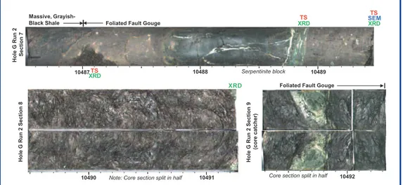
When the cores reached the surface, they were carefully cleaned, labeled, and photographed, and they have been stored at 4°C to prevent desiccation and microbial activity. The core is currently stored at the IODP Gulf Coast Repository (GCR) at Texas A&M University. High-resolution photographs and descriptions of all Phase 3 cores (as well as supplemental information including thin-section analysis, results from preliminary XRD analysis and core-log depth integration) are presented in a comprehensive Core Atlas (Table 1). One page of the core atlas is presented in Fig. 6, which shows a section of the core that crosses the SDZ. The foliated gouge matrix is highly altered, both chemically (e.g., there is much less silica and different clay mineralogy than observed in the rocks outside the fault zone) and mechani-cally (e.g., there is pervasive shearing observed on planes of varied orientation within the core). Clasts of various types of rock are seen in the gouge matrix, most notably clasts of serpentinite including a large piece of sheared serpentinite with calcite veins.
Zone (near or above the weight of the over- burden) has been one of the leading hypotheses to explain its low frictional strength (Rice, 1992). Two lines of evidence indicate an absence of severely elevated pore pressure (near-lithostatic, or greater) within the fault zone required to explain the low frictional strength of the San Andreas. Highly eleva-ted fluid pressures were not observed during drilling in the fault zone. Such pres-sures would have resulted in influxes of formation fluid into the wellbore if the pore pressure was appreciably greater than the drilling mud pressure. While the density of the drilling mud
was about 40% greater than hydrostatic pore to stabilize the borehole, in the strike slip/reverse faulting stress state that characterizes the SAFOD area (Hickman and Zoback, 2004), pore pressures within the deforming fault zone would have to exceed the overburden stress in Rice’s model (1992) for a weak fault in an otherwise strong crust. In addition, analysis of the rates of formation gas inflow during periods of no dril-ling (Wiersberg and Erzinger, submitted) shows no evi-dence of elevated pore pressure within the fault zone relative to the country rock, and the Vp/Vs ratio is relatively uniform (~1.7) across the ~200-m-wide damage zone and the local-ized shear zones within it (Fig. 4B). As Vp decreases seve-rely at very elevated pore pressure (i.e., at very low effective stress), Vs would not be affected as much, and the Vp/Vs ratio would be expected to decrease (Mavko et al., 1998). Altogether, none of these observations indicate the presence of anomalously high pore pressure in the fault zone.
Phase 3 – Coring the San Andreas Fault
Zone
During Phase 3 the SAFOD engineering and science teams successfully exhumed 39.9 meters of 10-cm-diameter continuous core, including cores from the two actively de-forming traces of San Andreas Fault Zone (the SDZ and CDZ; Zoback et al., 2010). Figure 5 shows the sidetracks drilled laterally off the SAFOD main borehole in map and cross-sectional views. Note the position of the cores with respect to the various contacts and shear zones described above. As shown, Core 1 was obtained close to the contact between the arkosic sandstones and conglomerates of the Salinian Terrane and the shales, mudstones and siltstones associated with the Great Valley Formation. The first
side-Figure 5. [A] Map view and [B] cross-section of the trajectory of the rotary-drilled SAFOD main borehole as it passed through the San Andreas Fault Zone at a depth of ~2700 m, as well as the trajectories of the sidetrack boreholes used to obtain core samples along the actively deforming traces of the fault during Phase 3. Note the positions of the SDZ, CDZ, and NBF and the extent of the damage zone as defined in Figs. 2, 3, and 4. Also shown are single-station locations of the aftershocks of the 11 August 2006 Hawaii target earthquake recurrence; these were made using a seismometer in the main hole at a true vertical depth of 2660 m. The “C” and “D” symbols refer to the polarity of the P-wave from each aftershock. Because the borehole seismometer is offset to the northeast from the fault trace, the transition from “C” to “D” occurs where expected for right lateral slip on the fault.
650 700 750 800 850
950
1000
1100
Easting (m)
Northing (m)
C C
C C
D D C
D C C
C CC C
C C C
C
C C C
C
1150 1250 1350
−2800
−2700
−2600
Cross-Section
North 45 East (m) True Vertical Depth (m) C
C C
C D D
C D CC
C CC C
C C
C C
C C C
C 3192 SDZ
SALINIAN TERRANE
SALINIAN
TERRANE
GREAT VALLEY FORMATION
Damage Zone
1050
GREAT VALLEY FORMATION
1200
3192 SDZ
3302 CDZ
3413
Core 1
Core 1
Core 2
Core 3
Core 3
SAFOD Main Borhole
SAFOD Main Borhole
Hawaii Aftershocks
Hawaii Aftershocks
SAFOD Observatory
Core 2
Damage Zone
SAFOD
3302 CDZ 3413 NBF
NBF
Observatory
crustal volume. Their results refined earlier tomographic models for SAFOD to clearly image a deep low-velocity zone along the San Andreas Fault. This low-velocity zone supports the propagation of both P- and S-type fault zone guided waves. Observation of these waves on seismometers placed inside the fault zone places strong constraints on its geometry and continuity. Ellsworth and Malin (in press) determined that the low-velocity zone in which these waves propagate coin-cides with the zone of extensive rock damage seen in the downhole measurements (Fig. 4). The waveguide extends to the northwest and southeast of SAFOD for at least 8 km. Wu et al. (2010) used the dispersion properties of the S-type guided waves recorded in the Main Hole to show that the low-velocity wave-guide extends downward to near the base of the seismogenic zone at 10–12 km depth.
The short hypocentral distances and high-Q environment of the SAFOD boreholes make it possible to study source parameters to smaller magnitude than with data from instru-ments in shallow boreholes or on the surface. Only a small fraction (<1%) of the San Andreas Fault surface near SAFOD produces earthquakes, with the remainder of the fault moving through aseismic creep. The earthquakes that do occur are predominately located within clusters of repeating events. Static stress drops range from as low as 0.1 MPa to 100 MPa (Imanishi and Ellsworth, 2006). The upper limit is comparable to the laboratory-derived frictional strength of the country rock from outside of the damage zone (Lockner et al., in press). McGarr and Fletcher (2010) determined the yield stress for a repeat of the SF target earthquake of 64 MPa. These results suggest that the target events and other repeating earthquakes occur where the fault juxtapo-ses normal crustal rocks patches embedded within an other-wise weak, creeping fault. As a consequence, there is no con-tradiction between such high stress drop events and an intrin-sically weak, creeping San Andreas Fault in a strong crust, as indicated by the in situ stress and heat-flow measu-rements in the SAFOD Pilot Hole and Main Hole.
The twenty-seven experi-mental deployments also guided the selection of sen-sors for the observatory and revealed mechanical and environmental issues that dictated the design of the observatory. The ambient temperature of up to 120°C at the planned depth of the observatory controlled the choice of downhole electro-nics and sensors. More seriously, the borehole fluid contains gases that penetrate past conventional O-rings and wireline insulation. Consequently, a design was To date, over 350 samples from the Phase 3 core have
been distributed to investigators from around the world for laboratory analyses and testing; the latest results from these studies were discussed at two SAFOD special sessions of the 2010 annual meeting of the American Geophysical Union. These include studies of the mineralogy and chemical evolu-tion of the fault zone, the physical properties of fault zone materials, the frictional strength of fault and country rock under a wide variety of loading conditions, and the evolution of deformation mechanisms and fluid-rock interaction within the fault zone over time. Procedures for requesting samples or gaining access to the SAFOD thin-section collection are available online (Table 1). The GCR staff is responsible for maintaining records of core, cuttings and fluid sample requests filled; names of people to whom these samples were provided; and the final disposition of samples (date samples returned and condition of samples). The GCR staff is also responsible for entering data and results from SAFOD sample investigations into the EarthScope Data Portal, which is currently under construction (Table 1).
SAFOD Observatory
In preparation for the establishment of a geophysical observatory deep within the fault, a series of nineteen temporary deployments of seismometers, accelerometers, and tiltmeters in the Main Hole and an additional eight deployments in the Pilot Hole were conducted between 2002 and 2008, leading up to the deployment of the SAFOD obser-vatory in September 2008 (data available online, Table 1).
Seismic data collected during the temporary deployments are yielding important new findings on the structure of the San Andreas Fault and properties of the earthquakes that it produces. By combining surface and borehole observa-tions of surface explosions and local earthquakes with double-difference tomography, Zhang et al. (2009) deter-mined a detailed Vp, Vs, and Vp/Vs model for the SAFOD
Ho
le
G
Ru
n
2
S
e
c
tio
n
7
10487 10488 10489
Massive,
Grayish-Black Shale Foliated Fault Gouge
Serpentinite block TS
XRD
TS
XRD
TS
SEM XRD
10490 Note: Core section split in half 10491
Ho
le
G
Ru
n
2
S
e
c
tio
n
8
XRD
Core section split in half 10492 Foliated Fault Gouge
Ho
le
G
Ru
n
2
S
e
c
tio
n
9
(c
o
re
c
a
tc
h
e
r)
~2.5 km from the array. The EM trace appears three times because the EM signal was recorded at three different gains. Note that the EM signal appears at the same time as the seis-mic waves. Hence, the EM signal is the result of shaking of the coil within the Earth’s magnetic field by the seismic waves as they pass the instrument.
selected that isolated all electrical and opti-cal control lines and all sensors from contact with the wellbore fluid. The system was desi-gned to be positively coupled to the casing and fully retrievable for maintenance when required.
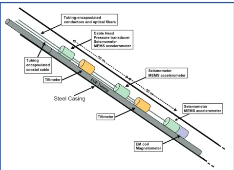
The installation of the SAFOD observa-tory was completed on 28 September 2008. The observatory instruments were deployed approximately 100 m above the Hawaii tar-get earthquake zone (Figs. 2, 5). As shown schematically in Fig. 7, the observatory instrumentation consisted of five pods con-taining different types of sensors. Pods 1 and 3 each contained a 3-component seismo-meter and a 3-component acceleroseismo-meter, Pods 2 and 4 each contained a 2-axis tilt-meter, and Pod 5 contained a 3-component seismometer and accelerometer as well as a passive electromagnetic (EM) coil. The goal of the EM ex-periment was to determine if
electromagnetic waves are radiated by the earthquake source. All of the instruments were housed in sealed steel pods that isolate them from contact with the wellbore fluids. The pods were attached to the outside of steel pipe (6-cm ‘EUE’ tubing) and coupled to the casing by decentralizing bow springs. The seismic and tilt systems were completely independent of each other, with separate power and data tele-metry lines encapsulated in 6.4-mm-diameter stainless steel tubing with pressure-tight connections in and out of the pods.
The seismic system was based on the Oyo Geospace DS150 digital borehole seismometer with a set of 3-component, 15-Hz Omni-2400 geophones in each sonde. MEMS accelerometers replaced the geophones in addi- tional DS150 units. The passive EM coil in Pod 5 was also digitized by a DS150. Fiber-optic telemetry was used to transmit the 4000-sample-per-second data from all seven DS150 units to the surface, where they were recorded on a USGS Earthworm computer system. The Earthworm system archived the data locally on LT3 tapes, downsampled se- lected channels to 250 samples per second and transmitted them to the Northern California Seismic Network (NCSN) where they were integrated into the real-time data system and archived at the Northern California Earthquake Data Center (NCEDC). Continuous full-sample-rate data are archived at the NCEDC and at the IRIS Data Management Center. The two borehole tiltmeters were manufactured by Pinnacle Technologies. Each tiltmeter produced two chan-nels of tilt data—recorded at one sample per 3 seconds— which were transmitted to the NCEDC for processing and archiving.
An example of the data produced by the SAFOD observa-tory instruments is shown (Fig. 8) for an earthquake located
Tiltmeter
Tiltmeter Tiltmeter
EM coil Magnetometer EUE
T
ubing
Tubing-encapsulated conductors and optical fibers
Tubing encapsulated coaxial cable
Cable Head Pressure transducer Seismometer MEMS accelerometer
Seismometer MEMS accelerometer
Seismometer MEMS accelerometer 50 m
50 m
Steel Casing
Figure 7. Schematic diagram of the instrumentation deployed in the SAFOD observatory above the location of the HI repeating earthquake sequence (see Fig. 5).
Figure 8. Seismograms from an M 1.3 microearthquake on 30 September 2008 recorded on the SAFOD observatory. The origin time of the microearthquake is shown by the dashed red line. The lower three traces are the output of the passive electromagnetic coil.
0.0 0.5 1.0 1.5 2.0 2.5 3.0
September 30, 2008 04:15:51 M 1.3
Seconds
Pod 1 Seis #1 Pod 1 Seis #2 Pod 1 Seis #1 Pod 1 Accel #1 Pod 1 Accel #2 Pod 1 Accel #1 Pod 3 Seis #1 Pod 3 Seis #2 Pod 3 Seis #1 Pod 3 Accel #1 Pod 3 Accel #2 Pod 3 Accel #1
Pod 5 Accel #1 Pod 5 Accel #2 Pod 5 Accel #1 Pod 5 Seis #1 Pod 5 Seis #2 Pod 5 Seis #1
then cemented in place. Each loop was anchored at the upper end at 9 m depth. One loop was anchored at the lower end at 864 m, and the other at 782 m, making strainmeters of 855 m and 773 m length, respectively. Although the longer loop failed in September 2007, vertical strain data continues to be produced from the shorter loop. Coseismic strain steps for local events have been reported by Blum et al. (2010) that are in general agreement with elastic dislocation theory.
Summary
We have already learned much about (i) the structure and physical properties of the fault zone at depth, (ii) the compo-sition of fault zone rocks, (iii) the stress, temperature, and fluid pressure conditions under which earthquakes occur, and (iv) the absence of deep-seated fluids in fault zone proc-esses. With the distribution of the Phase 3 core to research-ers around the world now underway, we can expect new insights into the physical and chemical mechanisms control-ling faulting and fault zone evolution within this major plate boundary fault. In addition, the observatory, even in its cur-rently reduced state, is providing high-quality near-field seismograms that may lead to novel observations of rupture nucle-ation and other insights into the nature of the earth-quake source and structure of the fault at seismogenic depth.
Acknowledgements
Scores of scientists, graduate students, engineers and technicians too numerous to name contributed immeasur-ably to the success of SAFOD. We would particularly like to thank Louis Capuano and Jim Hanson of ThermaSource, Inc., the prime drilling contractor, and the many individuals who served on the SAFOD Advisory Board and Technical Panels. We would especially like to thank Roy Hyndman of the Pacific Geoscience Center who served as Chair of the SAFOD Advisory Board. Funding for the project was provid-ed by the NSF’s EarthScope Program, with additional sup-port from the USGS, the ICDP, Stanford University, and NASA. Any use of trade, product, or firm names is for descriptive purposes only and does not imply endorsement by the U.S. government.
References
Almeida, R., Chester, J., Chester, F., Kirschner, D., Waller, T., and Moore, D., 2005. Mesoscale structure and lithology of the SAFOD Phase I and II core samples. Eos Trans. AGU, 86 (52), Fall Meeting Suppl., Abstract T21A-0451.
Bakun, W., and McEvilly, T., 1984. Recurrence models and Parkfield, California, earthquakes. J. Geophys. Res., 89(B5): 3051–3058.
Blum, J., Igel, H., and Zumberge, M., 2010. Observation of Rayleigh-wave phase velocity and coseismic deformation using an optical fiber, interferometric vertical strainmeter at the SAFOD Borehole, California. Bull. Seismol. Soc. Am., 100(5A):1879–1891, doi:10.1785/0120090333.
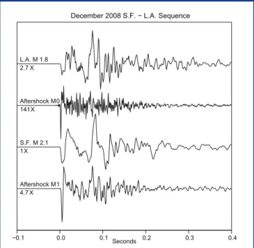
Unfortunately, the SAFOD observatory instruments began to develop electronic problems soon after installation, and attempts to keep the instruments running were ulti-mately unsuccessful. An expert panel convened by NSF is currently in the process of examining the failed instrumen-tation. Leakage of water into pods was the probable cause of failure, although the actual failure point will not be known until the NSF panel report is completed. Fortunately, the SAFOD observatory was designed to permit ongoing access to the deepest part of the Main Hole through the inside of the EUE tubing (Fig. 7) to which the instrument pods were attached. A seismometer with three 15-Hz Omni-2400 geo-phones was deployed on wireline inside the EUE tubing in early December 2008, and this continues to operate as of March 2011. Data are digitized at the surface at 1000 sam-ples per second and transmitted directly into the NCSN and are archived at the NCEDC (Table 1). While not a substitute for the observatory’s full suite of digital seismometers and accelerometers, this interim instrument has allowed contin-uous observation of the target earthquakes to continue, and has produced important data including recordings of the SF and LA target earthquakes repeat in December 2008 (Fig. 9). The temporary geophone is planned to remain in operation until NSF develops a plan for installation of a new observa-tory.
In addition to the SAFOD observatory, an optical-fiber interferometric strainmeter was permanently installed at the conclusion of Phase 1 drilling in 2004 (Blum et al., 2010). Two optical-fiber loops were placed in the annulus formed by the 311-mm inside diameter (ID) initial casing and the 245-mm OD casing. The fiber sensors were attached to the outside of the inner casing as it was lowered into the well and
Figure 9. Seismograms from an SF and LA repeating earthquake sequence that occurred in December 2008. This earthquake was recorded on a 3-component seismometer deployed within the EUE tubing at a position just above the SAFOD observatory.
−0.1 0.0 0.1 0.2 0.3 0.4
December 2008 S.F. − L.A. Sequence
Seconds L.A. M 1.8
Aftershock M 0
S.F. M 2.1
Aftershock M 1 2.7 X
141 X
1 X
![Figure 2. Microearthquakes selected for targeting with SAFOD. [A] 3-D perspective view of the seismicity with respect to the path of the SAFOD borehole, with north pointing up, east to the right, and depth down (all axes in km)](https://thumb-eu.123doks.com/thumbv2/123dok_br/18205203.333983/3.892.66.643.639.1004/figure-microearthquakes-selected-targeting-perspective-seismicity-borehole-pointing.webp)
![Figure 4. [A] Selected geophysical logs and generalized geology as a function of measured depth along the Phase 2 SAFOD borehole](https://thumb-eu.123doks.com/thumbv2/123dok_br/18205203.333983/9.892.67.552.352.954/figure-selected-geophysical-generalized-geology-function-measured-borehole.webp)
![Figure 5. [A] Map view and [B] cross-section of the trajectory of the rotary-drilled SAFOD main borehole as it passed through the San Andreas Fault Zone at a depth of ~2700 m, as well as the trajectories of the sidetrack boreholes used to obtain core sam](https://thumb-eu.123doks.com/thumbv2/123dok_br/18205203.333983/10.892.254.829.107.382/figure-trajectory-drilled-borehole-andreas-trajectories-sidetrack-boreholes.webp)